Controlling bi-partite entanglement in multi-qubit systems

Abstract

Bi-partite entanglement in multi-qubit systems cannot be shared freely. The rules of quantum mechanics impose bounds on how multi-qubit systems can be correlated. In this paper we utilize a concept of entangled graphs with weighted edges in order to analyze pure quantum states of multi-qubit systems. Here qubits are represented by vertexes of the graph while the presence of bi-partite entanglement is represented by an edge between corresponding vertexes. The weight of each edge is defined to be the entanglement between the two qubits connected by the edge, as measured by the concurrence. We prove that each entangled graph with entanglement bounded by a specific value of the concurrence can be represented by a pure multi-qubit state. In addition we present a logic network with $O(N^{2})$ elementary gates that can be used for preparation of the weighted entangled graphs of $N$ qubits.

1 Introduction

Motivated by the seminal paper of Einstein, Podolsky and Rosen (EPR) [1], Schrödinger in his paper entitled “The present situation in quantum mechanics” [2] has introduced a concept of entanglement. This new type of purely-quantum mechanical correlation has been introduced to reflect the fact that (according to Schrödinger) “Maximal knowledge of a total system does not necessarily include total knowledge of all its parts, not even when these are fully separated from each other and at the moment are not influencing each other at all.” Quantum correlations have attracted lot of attention during the history of quantum mechanics. Bell [3] and Clauser et al. [4] have shown that these correlations violate inequalities that must be satisfied by any classical local hidden variable model.

The complex phenomenon of quantum entanglement has been studied extensively in recent years because it represents an essential resource for quantum information processing (see, e.g. reference [5]). Entanglement between two qubits prepared in both pure and mixed states is well understood by now. In particular, necessary and sufficient conditions for the presence of entanglement in mixed two-qubit states have been derived [6, 7] and reliable measures of degree of entanglement have been introduced. Among others, the concurrence as introduced by Wootters et al. [8] is a very useful measure of entanglement since it is rather straightforward to calculate and is directly related to the entanglement of formation.

Entanglement properties in multi-qubit systems are, on the other hand, still not completely revealed. Firstly, intrinsic multi-partite entanglement is of a totally different nature then a “sum” of bi-partite correlations. Secondly, unlike classical correlations, bi-partite entanglement cannot be shared freely among many particles [9]. In particular, Coffman et al. have derived bounds on bi-partite concurrencies in three-qubit systems, which are referred to as CKW (Coffman-Kundu-Wootters) inequalities. Further investigation on entanglement sharing in multi-qubit systems have been reported in references [10, 11, 12, 13]. In these papers special states of multi-qubit systems that maximize bi-partite entanglement between selected pairs of qubits in the system have been presented. In addition, intrinsic multi-qubit quantum correlations have been analyzed (see, for instance, references [14, 15]).

Controlling the amount of shared bi-partite entanglement in multi-qubit systems can be used on multi-partite communication protocols such as quantum secret sharing [17] or specific multi-user teleportation schemes.

The entanglement properties of a multi-qubit system may be represented mathematically in several ways. Dür [13], for instance, has introduced entanglement molecules: mathematical objects representing distributions of bi-partite entanglement in a multi-qubit system. He has shown that given an entanglement molecule, relevant mixed states with the corresponding entanglement properties can be found.

An alternative possibility for representing the entanglement relations of a multi-qubit system is the application of entangled graphs. The entanglement properties of a system with $N$ qubits are represented by a graph of $N$ vertexes. The vertexes refer to the qubits, while the edges of the graph represent the presence of entanglement of the corresponding pairs of qubits. It was shown in one of our earlier papers [16] that for every possible graph one can find a pure state, which would be represented by that graph. The amount of pairwise entanglement was however not taken into account.

In the present paper we extend the concept of entangled graphs to describe the amount (degree) of pairwise entanglement in the system as well. Namely, we assign a weight to each edge of the graph, which is equal to the amount of the entanglement between the corresponding pair of qubits. The entanglement is quantified in terms of a concurrence.

For a given state of an $N$ qubit system, one can obviously calculate pairwise entanglement, thereby constructing the appropriate graph. The inverse problem, i.e. finding a quantum state with entanglement properties represented by a given graph, is more difficult.

In Sections 3 and 4 of the paper we will present a complete analysis of existence of quantum states of multi-qubit systems with entanglement properties represented by a given particular graph.

For a given graph, many quantum states may be appropriate per se. The graph itself is not, for instance, sensitive to local operations on the qubits. On the other hand, there exist graphs for which no suitable state can be found. The reason behind this is that bi-partite entanglement cannot be shared freely: e.g. the CKW inequalities form an obstacle. So, for instance, we cannot have an entangled graph of three qubits such that each pair is maximally entangled with the value of concurrence equal to unity. In spite of this, a positive statement can be made. We prove in the following, that if an additional criterion is fulfilled, namely that the weight of each edge is bounded from above by a certain value, a pure state corresponding to the given graph can be found. This bound on the weights depends only on the number of qubits in the system. We also propose a constructive method, how to find these states.

It is known that an arbitrary quantum state of $N$ qubits can be prepared using a sequence of single-qubit and two-qubit operations. These operations can formally be represented as a quantum logic network. In general one needs to use exponentially many resources (counted by the number of elementary gates) to prepare a quantum state of $N$ qubits.

We will show in Section 5, that for preparing a system of qubits in a state with given entanglement properties resulting from our consideration, less resources are needed. Namely, a quantum logic network composed of two- and three-qubit gates enables us to generate the state in argument. The number of gates building up this network is proportional to the number of entangled qubit pairs in the system (i.e. the edges of the graph). In the case of an entangled web for instance (c.f. reference [12]), when all vertexes of the graph are connected by edges, the number of gates necessary for a generation of the state is proportional to $N^{2}$.

2 Definitions

2.1 Concurrence

In this paper we will use concurrence as a measure of bi-partite entanglement. This has been introduced by Wootters et al. [8] in the following way: Let us assume a two-qubit system prepared in a state described by the density operator $\rho$. From this operator one can evaluate the so-called spin-flipped operator defined as

$$\tilde{\rho}=(\sigma_{y}\otimes\sigma_{y})\rho^{\ast}(\sigma_{y}\otimes\sigma_{y}),$$ (1)

where $\sigma_{y}$ is the Pauli matrix and a star (^∗) denotes the complex conjugation in the computational basis. Now we define the matrix

$$R=\rho\tilde{\rho}\,,$$ (2)

and label its eigenvalues (which are all non-negative), in decreasing order $\lambda_{1},\lambda_{2,}\lambda_{3}$ and $\lambda_{4}$. The definition of the concurrence is then

$$C={\rm max}\left\{0,\sqrt{\lambda_{1}}-\sqrt{\lambda_{2}}-\sqrt{\lambda_{3}}-\sqrt{\lambda_{4}}\right\}\,.$$ (3)

This function also serves as an indicator whether the two-qubit system is separable (in this case $C=0$), while for $C>0$ it measures the amount of bipartite entanglement between two qubits with a number between $0$ and $1$. The larger the value of $C$ the stronger the entanglement between two qubits is.

2.2 Coffman-Kundu-Wootters inequalities

Coffman et al. [9] have recently studied a set of three qubits, and have proved that the sum of the entanglement measured in terms of the squared concurrence between the qubits $1$ and $2$ and the qubits $1$ and $3$ is less than or equal to the entanglement between qubit $1$ and the rest of the system, i.e. the subsystem $23$. Specifically, using the bi-partite concurrence (3) the state $\varrho_{jk}$ between the qubits $j$ and $k$ we can express the Coffman-Kundu-Wootters (CKW) inequality as

$$C_{12}^{2}+C_{13}^{2}\leq C^{2}_{1,(23)}\,.$$ (4)

Coffmann, Kundu and Wootters have conjectured that a similar inequality might hold for an arbitrary number $N$ of qubits prepared in a pure or mixed state. That is, one has

$$\sum_{k=1;k\neq j}^{N}C^{2}_{j,k}\leq C^{2}_{j,\overline{j}}\,,$$ (5)

where the sum on the left-hand-side is taken over all qubits except the qubit $j$, while $C^{2}_{j,\overline{j}}$ denotes the concurrence between the qubit $j$ and the rest of the system (denoted as $\overline{j}$). The maximal value of the concurrence $C^{2}_{j,\overline{j}}$ at the right-hand side of equation 5 is equal to unity.

2.3 Entangled graphs

Let us consider a system of $N$ qubits. As already mentioned, we will represent the entanglement properties of the system with a weighted graph with $N$ vertexes. Every qubit is identified with one of the vertexes, whereas the concurrence between a pair of qubits is identified with a weighted edge, connecting relevant vertexes. If a pair of qubits is not entangled at all, there is no edge present in the graph between the relevant vertexes (thus, the edge with a zero weight is equivalent to no edge). The graph itself is defined by the number of qubits $N$ and a set of real numbers $C_{ij}$, giving the concurrencies between relevant pairs of qubits.

3 Simple examples

The simplest example of a multi-qubit system with interesting correlation properties was studied in the work of Koashi et al. [12]. These authors have studied a completely symmetric state of $N$ qubits such that all $N(N-1)/2$ pairs of qubits in the system are entangled with the same degree of entanglement. It has been shown that a state satisfying this condition is the so-called $W$-state defined as

$$|W\rangle=|N;1\rangle,$$ (6)

where $|N;k\rangle$ is a totally symmetric state of $N$ qubits, with $k$ qubits in the state $|1\rangle$ and all the others in the state $|0\rangle$. The concurrence in this case takes the value

$$C_{\max}=\frac{2}{N},$$ (7)

that is maximal under given conditions.

One can easily generalize this example for other completely symmetric configurations (e.g. for graphs with weights equal on all edges). As proved by Koashi et al. [12], if the value of concurrence is larger than $2/N$ [see equation (7)], then the desired state does not exist. If it is smaller than $2/N$ then a pure state corresponding to the desired entangled web reads

$$|\Psi\rangle=\sqrt{1-\alpha^{2}}|N;0\rangle+\alpha|N;1\rangle\,.$$

The desired value of the concurrence $C$ determines the value of a real parameter $\alpha$ which reads

$$\alpha=\sqrt{\frac{CN}{2}}=\sqrt{\frac{C}{C_{\max}}}\,.$$

A more complicated two-parameter example is the case of a star-shaped entangled graph (see reference [18]). In this graph a given qubit is entangled with all the other qubits in the system while no other qubits are entangled between themselves. In addition, it is assumed that the strength of the entanglement between the given qubit and any other qubit is the same (constant). In the reference [18] it has been shown, that asymptotically, in the limit of large number of qubits (i.e. $N\to\infty$), one is able to find a state that saturates the CKW inequalities. Thus we are able to find a state for every star-shaped graph in the $N\rightarrow\infty$ limit .

4 General solution

As we have mentioned earlier, it has been conjectured, that all $N$-qubit states have to fulfil the Coffman-Kundu-Wootters (CKW) inequalities (see equation (5)) which in the case when the qubit $j$ is maximally entangled with the rest of the system reads

$$\forall~{}j,\quad\sum_{k}C_{kj}^{2}\leq C^{2}_{j,\overline{j}}\leq 1\,.$$ (8)

Any violation of this inequality means that the corresponding entangled graph cannot be represented by a quantum-mechanical state. Under the assumption that all concurrencies $C_{kj}$ in equation (8) are mutually equal, i.e. $C\equiv C_{kj}$, we obtain from the CKW inequality the bound

$$C\leq\frac{1}{\sqrt{N}}$$

which is definitely not achievable. To see this we remind ourselves, that in the case of the entangled web (all qubits are mutually entangled) the maximal value of the concurrence is given by equation (7), which represents a bound that is much lower than the bound that follows from the CKW inequality.

One may proceed either by deriving tighter CKW-type inequalities that can be saturated by physical states (graphs). Alternatively, one can consider only entangled graphs with specifically bounded weights on their edges. In what follows we will study this second option and will restrict the consideration to those graphs in which the concurrence on every edge is smaller than a certain value. We will prove that there exists a nonzero bound on the concurrence such that all graphs with weighted edges that satisfy this additional condition can be realized by pure states.

These states are of the form

$$|\Psi\rangle=\alpha|A\rangle+\sum_{\{i,j\}}\gamma_{ij}|B_{ij}\rangle$$ (9)

where

$$|B_{ij}\rangle \equiv \left(|11..0_{i}..0_{j}..1\right\rangle+\left|00..1_{i}..1_{j}..0\rangle\right)\,;$$ (10)

$$|A\rangle \equiv \left(\left|00...0\right\rangle+\left|11...1\right\rangle\right)\,.$$ (11)

The real positive coefficients $\alpha$ and $\gamma_{ij}$ satisfy a normalization condition

$$2\alpha^{2}+2\sum_{\{i,j\}}\gamma_{ij}^{2}=1.$$ (12)

The sums in equations (9) and (12) are taken through all pairs $i<j,$ $i,j\in N$ (or, equivalently, the sums can be extended for all pairs $i,j\in N$ with the restriction $\gamma_{ij}=0$ for $j\leq i$). The high (permutational) symmetry of the state allows us to calculate directly the concurrence (for details see Appendix A)

$$C_{ij}=\max\left\{2{\left(2\alpha\gamma_{ij}-\sum_{k}\gamma_{ki}^{2}-\sum_{k}\gamma_{kj}^{2}\right),0}\right\},$$ (13)

which is valid under the condition

$$\alpha\geq 2\gamma_{\max}\sqrt{N-2}\,,$$ (14)

where $\gamma_{\max}=\max_{i,j}(\gamma_{ij})$.

Let us note, that the concurrence between every pair of qubits in this rather complex system is expressed as an analytic function of input parameters, utilizing just a single condition (14).

The set of $\frac{N(N-1)}{2}$ non-linear equations (13) connect parameters of the state $\gamma_{ij}$ (the parameter $\alpha$ is specified by gammas via the normalization condition) with the concurrencies of different pairs of qubits. This set of equations is strongly coupled in a sense that in order to calculate one concurrence one needs to use approximately $2N$ gammas. The task now is to invert this set of equations, i.e. to find the set of equation defining the gammas via the set of concurrencies that are given (these concurrencies do specify the character of the entangled graph). Not for every possible choice of concurrencies there exist parameters $\gamma_{ij}$ satisfying the normalization condition $\Sigma_{i,j}\left|\gamma_{ij}\right|^{2}<1$ and the condition (14). The reason is that even though the concurrencies under consideration have to fulfil the CKW inequalities these inequalities are just necessary but sufficient condition for the existence of an entangled graph with weighted edges. Hence, it is also an interesting question, for which set of concurrencies one can find solutions of the reversed equations (13).

We have found the solution for the parameters $\gamma_{ij}$ as functions of the concurrencies $C_{ij}$ (weights on the edges of the entangled graph) that specify the state (9), providing all concurrencies are smaller than a certain maximal value

$$C_{ij}\leq C_{\max},$$ (15)

where $C_{\max}$ is a given constant. .

Theorem 1
Every entangled graph with weighted edges that is specified by the set of concurrencies $\{C_{ij}\}$, that fulfil the condition (15), can be represented by a pure state given by equation (9)

The complete proof of this Theorem can be found in Appendix B. Here we just sketch how the relevant parameters $\gamma_{ij}$ can be obtained via an iteration algorithm. Let us start from a specific state (9) corresponding to the situation when

$$C_{ij}=C_{\max}$$

for all $i,j$ and then adjusts iteratively the parameters $\gamma_{ij}$ to fit the concurrencies. We can summarize the iteration process as follows:

• After each step, all concurrencies that are evaluated for the state (9) are greater than or equal to the desired set of concurrencies $C_{ij}$.

• After each step, all gammas are smaller than or equal to their values at the previous step; they do not change only if for a specific $i,j$ the relevant concurrence is reached.

• The iteration limit, when all gammas are zero, leads to zero concurrencies, too. Therefore, one has to cross the searched state during the iteration procedure (for a finite precision this stage can be achieved after a finite number of iteration steps)

The existence of the state itself is proved by showing, that the iteration process has a proper limit. Also, to ensure the validity of the proposed process, we made a broad numerical test, with varying number of qubits and the strength of entanglement. In all tested examples that satisfied the condition (15), a very rapid convergence was observed, when a precision of about $10^{-6}$  of the maximal permitted concurrence was achieved after nine to twelve steps (changing all gammas at once).

5 Preparation of entangled graph with weighted edges

In the previous section we have shown that a large class of entangled graphs with weighted edges can be represented by a pure state (9). It is well known (see e.g. Ref. [5]) that any state of a multi-qubit system can be prepared with the help of a suitable logic network. However, in general the number of two-qubit gates in this network increases exponentially with the number of qubits.

In what follows we present a quantum logic network for preparation of the state (9), corresponding to a given weighted entangled graph. This network is very efficient in a sense that it uses only a quadratic number of three-partite gates with respect to the number of qubits (every three-qubit gate can be decomposed in at most eight two-qubit gates). Three ancilla qubits are needed for the procedure; these are not entangled with the other ones at the end of the preparation process. This keeps the fidelity of the preparation (in the case of error-free gates) perfect.

5.1 Definitions

Firstly let us introduce logic gates that will be used in our network. The first gate is a two-qubit operator, the well-known controlled NOT ($cNOT$) gate. In this gate the first input qubit serves as a control. The NOT operation is applied on the second qubit when the control qubit is in the state $\left|1\right\rangle$, otherwise the second qubit does not change. The operator which implements this gate acts on the basis vectors of the two qubits under consideration as follows

$$cNOT\left|0\right\rangle_{i}\left|0\right\rangle_{j} = \left|0\right\rangle_{i}\left|0\right\rangle_{j}$$ (16)

$$cNOT\left|0\right\rangle_{i}\left|1\right\rangle_{j} = \left|0\right\rangle_{i}\left|1\right\rangle_{j}$$

$$cNOT\left|1\right\rangle_{i}\left|0\right\rangle_{j} = \left|1\right\rangle_{i}\left|1\right\rangle_{j}$$

$$cNOT\left|1\right\rangle_{i}\left|1\right\rangle_{j} = \left|1\right\rangle_{i}\left|0\right\rangle_{j},$$

where $i$ denotes the control and $j$ the target qubit.

The second gate we are going to use is a three-qubit Toffoli gate $T$ with two control qubits. In the case that these two control qubits are in the state $\left|11\right\rangle$ then the NOT operation is applied on the third qubit. In all other cases the Toffoli gate acts as an identity operator.

The third gate we will use is also a three-qubit gate, denoted as $R\left(\alpha\right)$. Here one qubit will serve as a control. When this control qubit is in the state $|1\rangle$ then a specific “rotation” in the two-dimensional subspace of the Hilbert space of the two target qubits will be applied. This rotation acts on the two target qubits as follows:

$$R\left(\alpha\right)\left|00\right\rangle = \left(1-\left(\alpha\right)^{2}\right)^{1/2}\left|00\right\rangle-\alpha\left|11\right\rangle\,;$$ (17)

$$R\left(\alpha\right)\left|11\right\rangle = \alpha\left|00\right\rangle+\left(1-\left(\alpha\right)^{2}\right)^{1/2}\left|11\right\rangle\,;$$

$$R\left(\alpha\right)\left|01\right\rangle = \left|01\right\rangle\,;$$

$$R\left(\alpha\right)\left|10\right\rangle = \left|10\right\rangle,$$

where $\alpha$ is a parameter of the rotation.

The last gate that will be used in our network is a three-qubit gate, which will be denoted by $A$. Again, one qubit serves as a control. The following transformation is applied to the two remaining qubits when the control qubit is in the state $\left|1\right\rangle$:

$$A\left|00\right\rangle = k_{+}\left|00\right\rangle-k_{+}\left|01\right\rangle-k_{-}\left|10\right\rangle+k_{-}\left|11\right\rangle\,;$$ (18)

$$A\left|01\right\rangle = k_{-}\left|00\right\rangle+k_{+}\left|01\right\rangle-k_{-}\left|10\right\rangle+k_{+}\left|11\right\rangle\,;$$

$$A\left|10\right\rangle = k_{+}\left|00\right\rangle+k_{-}\left|01\right\rangle+k_{+}\left|10\right\rangle-k_{-}\left|11\right\rangle\,;$$

$$A\left|11\right\rangle = -k_{-}\left|00\right\rangle-k_{-}\left|01\right\rangle+k_{+}\left|10\right\rangle+k_{+}\left|11\right\rangle\,,$$

where we have used a short-hand notation $k_{\pm}=\frac{1}{2}\sqrt{1\pm\frac{1}{\sqrt{2}}}$. This operation will be used in our network even number of times, so only the effects of the operation $A^{2}$ will appear at the end. The operation $A^{2}$ acts in a simpler and understandable way

$$A^{2}\left|00\right\rangle = -\left|01\right\rangle\,;$$ (19)

$$A^{2}\left|01\right\rangle = \left|11\right\rangle\,;$$

$$A^{2}\left|10\right\rangle = \left|00\right\rangle\,;$$

$$A^{2}\left|11\right\rangle = \left|10\right\rangle\,.$$

5.2 Initial state of the $N$ qubits

In order to prepare an entangled graph with $N$ vertexes, i.e. a specific $N$-qubit state, we will need three additional ancilla qubits. The ancilla is initially prepared in the product state $|1\rangle|0\rangle|0\rangle$ and is completely factorized from the other, graph qubits. These graph state are initially prepared in the generalized Greenberger-Horne-Zeilinger (GHZ) state $(\left|\Psi\right\rangle_{I}=|1\rangle^{\otimes N}-|0\rangle^{\otimes N})/\sqrt{2}$. Thus the input state of the quantum logic network under consideration reads

$$\left|\Psi\right\rangle_{I}\left|1\right\rangle_{N+1}\left|0\right\rangle_{N+2}\left|0\right\rangle_{N+3}=\frac{1}{\sqrt{2}}\left(\left|11...1\right\rangle-\left|00...0\right\rangle\right)\left|1\right\rangle_{N+1}\left|0\right\rangle_{N+2}\left|0\right\rangle_{N+3}.$$ (20)

In what follows we will specify gates in the network with three indices, where the first index specifies the control qubit (or the first two qubits in the case of the Toffoli gate) and remaining index(es) determine(s) the target qubit(s) of the operation. In addition, if there will be some action or control applied on the ancillas, we will denote their relevant indexes as $N+i$, where $i=1,2,3$ is the position of the ancilla qubit.

5.3 The network

The action of the network can be divided into two main stages. In the first stage an entangled state of the graph qubits and the ancilla is created. This state contains state vectors that are essentially the same as those in the desired state (9). In the second stage of the preparation procedure the ancilla becomes factorized from the graph, which in turn is prepared in the state (9).

During the first stage of the preparation procedure we will apply the rotation $R\left(\alpha_{ij}\right)$ to each pair $i\neq j$ from $N$ target qubits with the control on the first ancilla qubit (see Figure 1).

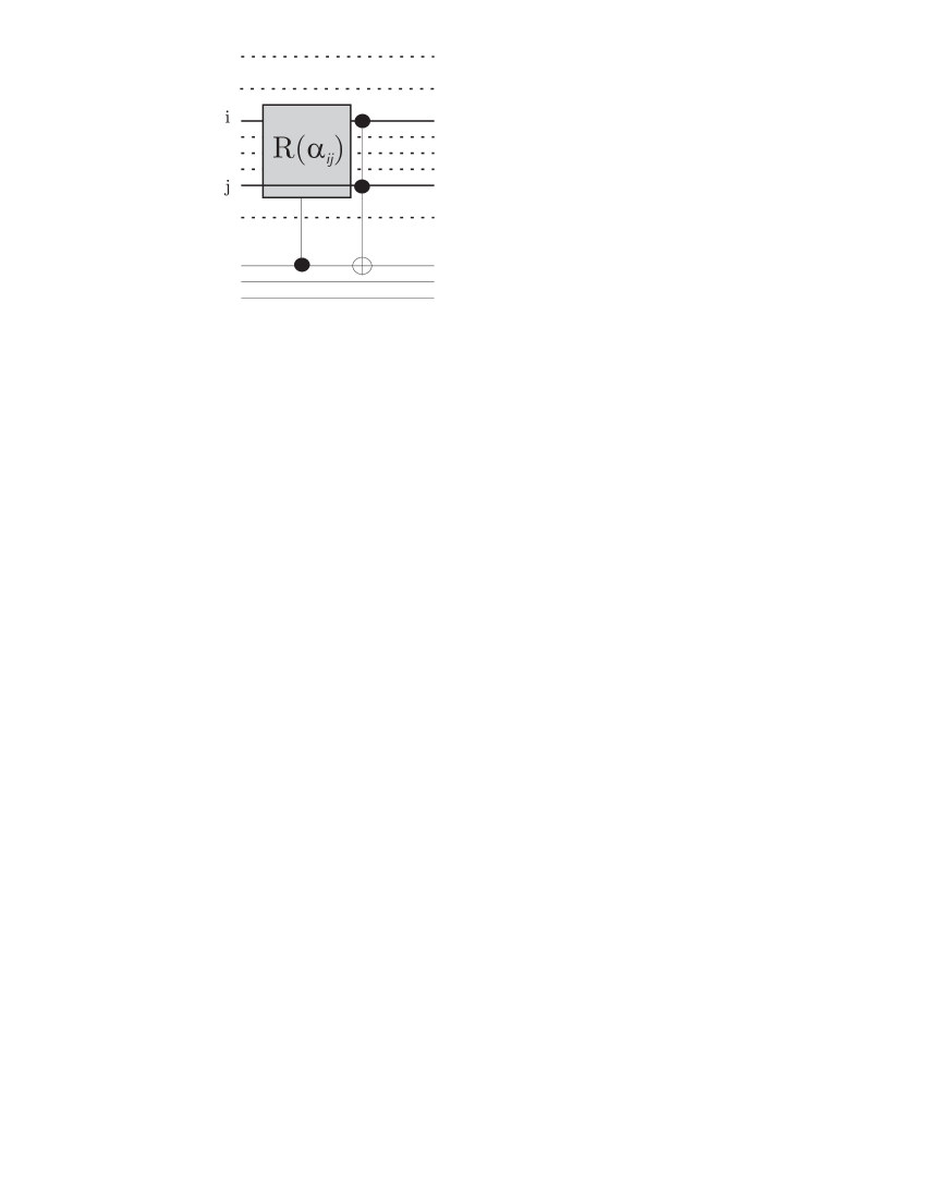
Figure 1: A schematic description of the logic network corresponding to the first stage of the preparation procedure. The rotation $R(\alpha)$ is applied on every pair of the target qubits (all original qubits, except the ancilla qubits), with $\alpha$ defined by the parameters $\gamma_{ij}$ that specify the state corresponding to a given entangled graph. During this first stage of the preparation procedure approximately $N^{2}$ elementary gates are used.

After each $R\left(\alpha_{ij}\right)$-gate the Toffoli gate with the control on $i$ and $j$ qubits acts on the $first$ ancilla qubit. This procedure is repeated ${N\choose 2}$-times, for all indices $i\neq j$. During each rotation, a fraction (that is specified by the amplitude $\alpha_{ij}$) of the state vector $\left(\left|11...1\right\rangle-\left|00...0\right\rangle\right)$ is transformed into the state $\left(\left|11..0_{i}..0_{j}..1\right\rangle+\left|00..1_{i}..1_{j}..0\right\rangle\right)$, whereas the already transformed part of the state $\left(\left|11..0_{k}..0_{l}..1\right\rangle+\left|00..1_{k}..1_{l}..0\right\rangle\right)$ is left unchanged.

Thus, after a few steps the state given by equation (20) is transformed into

$$\left|\Psi\right\rangle = \widetilde{\sum_{\{i,j\}}}E_{ij}\left(\left|11..0_{i}..0_{j}..1\right\rangle+\left|00..1_{i}..1_{j}..0\right\rangle\right)\left|0\right\rangle\left|0\right\rangle\left|0\right\rangle$$

$$+D\left(\left|11...1\right\rangle-\left|00...0\right\rangle\right)\left|1\right\rangle\left|0\right\rangle\left|0\right\rangle,$$

where the tilde indicates that the sum is taken over all pairs of qubits that have already been involved in the transformation. The corresponding amplitudes $C_{ij}$ are given by the relation

$$E_{ij}=\frac{\alpha_{ij}}{\sqrt{2}}\left(1-2\widetilde{\sum_{\{k,l\}}}E_{kl}^{2}\right)^{\frac{1}{2}}$$ (22)

and $D$ is given by the normalization condition.

We have also to specify the parameters $\alpha_{ij}$ for each rotation. These parameters are related to amplitudes $\gamma_{ij}$ that specify the desired state of the entangled graph given by equation (9), which we want to generate. Comparing the states (9) and (5.3) we see, that for a successful generation of the state of the graph we need $E_{ij}=\gamma_{ij}$. Using equation (22) we can write

$$\alpha_{ij}=\sqrt{2}\left(1-2\widetilde{\sum_{\{k,l\}}}\gamma_{kl}^{2}\right)^{-\frac{1}{2}}\gamma_{ij}.$$ (23)

After performing transformations on all pairs of target qubits the resulting state has the form

$$\left|\Psi\right\rangle=\sum_{\{i,j\}}\gamma_{ij}|B_{ij}\rangle\left|0\right\rangle\left|0\right\rangle\left|0\right\rangle+\alpha\left|\overline{A}\right\rangle\left|1\right\rangle\left|0\right\rangle\left|0\right\rangle.$$ (24)

where the state vector $|B_{ij}\rangle$ is given by equation (10) and

$$|\overline{A}\rangle \equiv \left(\left|11...1\right\rangle-\left|00...0\right\rangle\right)\,.$$ (25)

We see that the component states $|B_{ij}\rangle$ and $|\overline{A}\rangle$ in equation (24) are essentially the same as those of the desired entangled graph (see equation (9)). Now we will use the first ancilla qubit the last time before disentangling it from the rest of the system. We will apply the specific controlled rotation on an arbitrary qubit of the graph with the control being the first qubit of the ancilla. The rotation itself is described by the operator $-\sigma_{z}$ (a Pauli matrix). This controlled rotation applied on the state (24) performs the transformation $|\overline{A}\rangle\rightarrow|A\rangle$, while the state $|B_{ij}\rangle$ remains unchanged.

We see that at this stage the two desired components $\alpha|A\rangle$ and $\sum\gamma_{ij}|B_{ij}\rangle$ of the graph state (9) are generated, but they are entangled with the first ancilla qubit. The second stage of the preparation procedure is designed so that the ancilla is disentangled from the graph, while the graph is left in the state (9). To disentangle the first ancilla qubit from the rest of the system we will use the other two ancilla qubits. In order to perform this disentanglement we have to find a network that will discriminate between two graph states $|A\rangle$ and $\sum\gamma_{ij}|B_{ij}\rangle$

Let us analyze in more detail the state $\sum\gamma_{ij}|B_{ij}\rangle$. In this state two or four neighboring qubits are in different states. This is in contrary to the state $|A\rangle$, in which all qubits are in the same state. The discrimination of the two states can so be performed by applying the $cNOT$ gate acting always on two neighbouring qubits. If the target is in the state $\left|0\right\rangle$ then after the action of the $cNOT$ gate the two qubits that are involved in the action of the gate are in the same state. On the other hand, if it is $\left|1\right\rangle$, the two qubits do differ. From here it follows that we can use the target qubit as a control for another gate, which changes its targets if and only if the two graph qubits do differ.

Let us utilize for this purpose the gate $A$ which will act on the last two ancillas (see Figure 2).

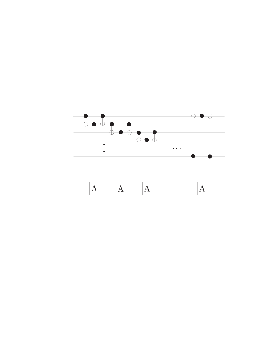
Figure 2: This part of the network helps to disentangle the ancilla qubits from the original qubits. In this case, the rotation $A$ is applied only in the case, when two neighboring qubits are not equal. Only $N$ elementary gates, in the order of the magnitude, are used.

We apply the $cNOT$ gate on two qubits from $N$ graph qubits and then we apply the $A$-gate controlled by the target of the $cNOT$, acting on the last two ancillas. After that, we apply again the $cNOT$ gate on the same two qubits as before: This operation will bring all qubits into the original state (since $cNOT^{2}=I$) and the only effect of this particular procedure is a rotation of the state of the last two ancillas. This rotation will take place only in the case when the two “tested” qubits were in a different state.

Than we repeat the same procedure for each pair of the first $N$ neighboring qubits of the graph. After this, the $A$ gate acted either $2$ or $4$ times on ancilla qubits, that are entangled with the state $\sum\gamma_{ij}|B_{ij}\rangle$ of the graph. On the other hand those ancillas that are entangled with the state $|A\rangle$ are not changed.

The reason for using $A$-gate, the “square root” of the operation (19), now becomes clear: the $A^{2}$ gate is acting once or twice and the state $\left|0\right\rangle\left|0\right\rangle$ of the last two ancillas is changed either to $-\left|0\right\rangle\left|1\right\rangle$ or to $\left|1\right\rangle\left|1\right\rangle$. On the other hand in the case when all target qubits are equal, $A$ will not act at all and the resulting state of the last two ancillas will be unchanged, thus $\left|0\right\rangle\left|0\right\rangle$. If the $cNOT$ gate between the last (control) and the first (target) ancilla qubit is applied, then the first ancilla will be changed to the state $\left|0\right\rangle$ and it becomes disentangled from the rest of the system. Now all the work is almost done, the only thing we have to do is to disentangle the two remaining ancilla qubits. For this we will simply run the procedure for all neighboring pairs of qubits as described above, but with the gate $A^{-1}$ instead of the gate $A$. This will change the state of the last two ancilla qubits back to the original state $\left|0\right\rangle\left|0\right\rangle$ and will finally disentangle the ancilla from the system. That means that the desired state $|\Psi\rangle$ of the $N$ graph qubits is disentangled from the ancilla and the entangled graph is prepared in the state (9).

Finally, let us summarize the preparation procedure for the entangled graph given by the state (9). As shown in Figure 3,

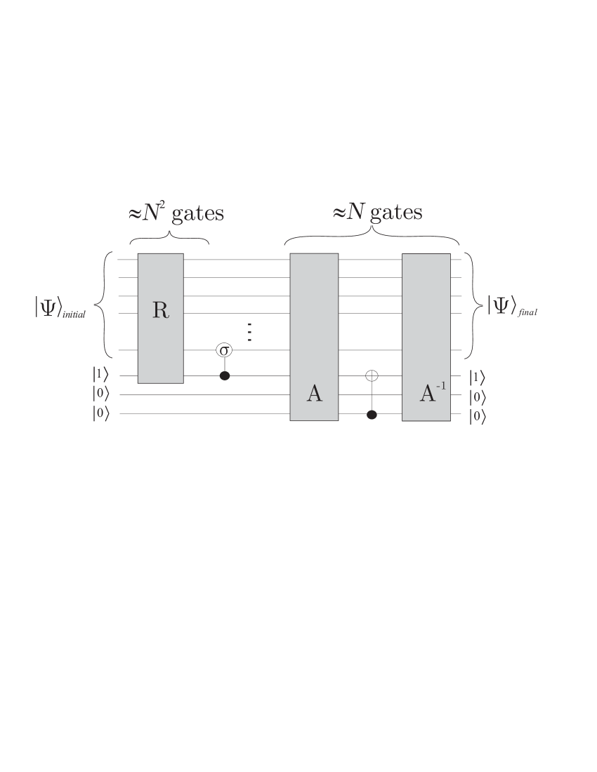
Figure 3: A schematic description of the entire logic network for the preparation of the entangled graph in the state (9). First we use the part with the rotation $R(\alpha)$, then we correct a sign with the help of a $cNOT$ gate. Finally, we disentangle the ancilla qubits with the help of the $A$ and $A^{-1}$ rotations. The desired state is prepared with the help of (of the order of magnitude) $N^{2}$ elementary gates.

first we apply the rotations $R$ on all pairs of qubits of the graph, i.e.

$$G_{1}=\left(c\sigma_{z}\right)_{N+1,N}\prod_{i\neq j}\left(T_{i,j,N+1}R\left(\alpha_{ij}\right)_{N+1,i,j}\right),$$ (26)

where the subscripts for each operation define the position of qubits, where operation takes its action. Angles of rotations $\alpha_{ij}$ are defined by equation (23) and $c\sigma_{z}$ stands for the controlled sigma gate applied on the first ancilla as a control and one of the graph qubits as a target. At this stage we will use roughly $N^{2}$ bipartite gates. The second stage of the preparation corresponds to disentangling the first ancilla qubit from the graph qubits

$$G_{2}=cNOT_{N+3,N+1}\prod_{i,i+1}^{N}\left(cNOT_{i,i+1}A_{i+1,N+2,N+3}cNOT_{i,i+1}\right)\,.$$ (27)

The last stage of the preparation process is responsible for disentanglement of the last two ancilla qubits from the graph qubits, i.e.

$$G_{3}=\prod_{i,i+1}^{N}\left(cNOT_{i,i+1}{A^{-1}}_{i+1,N+2,N+3}cNOT_{i,i+1}\right).$$ (28)

In the last two equations the indices $i+1$ for the gates are taken implicitly as modulo $N$. Finally we can represent the action of the whole logic network as

$$|\Psi\rangle_{F}|1\rangle_{N+1}|0\rangle_{N+2}|0\rangle_{N+3}=G_{3}.G_{2}.G_{1}.|\Psi\rangle_{I}|1\rangle_{N+1}|0\rangle_{N+2}|0\rangle_{N+3},$$ (29)

where $|\Psi\rangle_{F}$ is the desired state (9) of the entangled graph with weighted edges.

6 Conclusion

In this paper, we have introduced a concept of entangled graphs with weighted edges. Using simple examples we have shown, that sharing of bipartite entanglement is a complicated phenomenon and that the Coffman-Kundu-Wootters inequalities [9] are only a necessary condition for an existence of states with given entanglement properties.

We have proved that a whole class of entangled graphs, where the concurrence between an arbitrary pair of qubits (vertexes) is weaker than a certain value can be realized by a state of $N$ qubits. Moreover, we have proposed a logic network for preparation of the states corresponding to this entangled graphs. The network is composed of a number of elementary quantum gates that grows quadratically with the number of vertexes (qubits) in the graph.

Appendix A Concurrence in entangled graphs

In what follows we will evaluate the concurrence between an arbitrary pair of qubits of a system in the state (9), i.e.

$$|\Psi\rangle=\alpha\left(|00...00\rangle+|11...11\rangle\right)+\sum_{\{i,j\}}\gamma_{ij}\left(|11\rangle_{ij}|00...00\rangle_{\overline{ij}}+|00\rangle_{ij}|11...11\rangle_{\overline{ij}}\right)\;,$$ (30)

where real positive amplitudes $\alpha$ and $\gamma_{ij}$ satisfy the normalization condition

$$2\alpha^{2}+2\sum_{\{i,j\}}\gamma_{ij}^{2}=1.$$ (31)

The sum in equations (30) and (31) is taken through all pairs $i\neq j,$ $i,j\in\hat{N}$, so $\{i,j\}=\{j,i\}$ and thus $\gamma_{ij}=0$ for $i<j$. The special form of the state (30) leads to a rather compact density matrix for an arbitrary two-qubit operator that is obtained by tracing over the rest of the graph qubits:

$$\rho_{ij}=\left(\begin{array}[]{cccc}A&0&0&F\\ 0&B&E&0\\ 0&E&B&0\\ F&0&0&A\end{array}\right)\;,$$ (32)

where we have used the notation

$$A = \gamma_{ij}^{2}+\alpha^{2}+\sum_{\{k,l\}}\gamma_{kl}^{2}\,;$$ (33)

$$B = \sum_{k}\left(\gamma_{kj}^{2}+\gamma_{ki}^{2}\right)\,;$$

$$E = 2\sum_{k}\gamma_{ki}\gamma_{jk}\,;$$

$$F = 2\alpha\gamma_{ij}\,.$$

All sums in equations (33) are running through free parameter(s) $k$ (and $l$), whereas $i$ and $j$ denote a specific pair of qubits in the graph. In addition, the condition $i\neq k\neq l\neq j$ has to be fulfilled.

The convenient form of the matrix (32) allows us to calculate square roots of the eigenvalues of the matrix $R$ given by equation (2):

$$\lambda_{1} = A+F\,;$$ (34)

$$\lambda_{2} = A-F\,;$$

$$\lambda_{3} = B+E\,;$$

$$\lambda_{4} = B-E\,.$$

Because the coefficients $A,B,E,F$ are positive, the only candidates for the largest eigenvalue are $\lambda_{1}$ and $\lambda_{3}$. Let us further define

$$\gamma_{\max}=\max_{i,j}(\gamma_{ij})\,.$$ (35)

Using the condition

$$\alpha\geq 2\gamma_{\max}\sqrt{N-2}$$ (36)

we find $\lambda_{1}\geq\lambda_{3}$ and the general expression for the concurrence associated with edges of the entangled graph prepared in the state (30) reads

$$C_{ij}=\max\left\{2{\left(2\alpha\gamma_{ij}-\sum_{\{k,i\}}\gamma_{ki}^{2}-\sum_{\{k,j\}}\gamma_{kj}^{2}\right),0}\right\}.$$ (37)

Appendix B Proof of Theorem 1: Iterative procedure

In order to prove Theorem 1 we first label the set of concurrencies that determine a given entangled graph by ${\bf C}_{ij}$. We will use a bold C in order to distinguish these concurrencies from any intermediate concurrencies, obtained by searching for the state of the entangled graph.

We will start the iteration procedure with an initial state of the entangled graph given by equation (9). The amplitudes $\gamma_{ij}$ are specified by the relation

$$\gamma_{ij}^{(0)}\equiv\frac{\lambda}{\sqrt{2+N(N-1)\lambda^{2}}}\,,$$ (38)

that is, the initial state is completely permutationally symmetric. The parameter $\lambda$ is defined as

$$\lambda=\frac{\sqrt{4(N-2)^{2}+2N(N-1)}-2(N-2))}{N(N-1)}.$$ (39)

The corresponding bi-partite concurrencies can be evaluated straightforwardly and they read:

$$C_{ij}^{(0)} = C_{\max}=2\left(\alpha^{(0)}\gamma_{ij}^{(0)}-2(N-2)(\gamma_{ij}^{(0)})^{2}\right)$$ (40)

$$= \frac{\sqrt{6N^{2}-18N+16}-2N+4}{N(N-1)}{}\,.$$

We remind ourselves that the parameters $\alpha^{(0)}$ and $\gamma_{ij}^{(0)}$ are mutually related via the normalization condition (12), therefore $\alpha$ is always implicitly defined by $\gamma_{ij}$. It is also clear that for the state under consideration the condition (14) is fulfilled as well.

Before we describe the iteration procedure itself we introduce the following notation: we enumerate all pairs of qubits in the entangled graph. All pairs of qubits (i.e. the edges of the graph) are listed in the set of pairs just once. At each iteration step one parameter $\gamma_{kl}$ for a selected pair of indices $\{k,l\}$ is changed, whereas all others gammas will stay unchanged. Let us now suppose, that the $n$-th step of the iteration is done and both conditions (15) and (14) are still fulfilled. Moreover $\alpha^{(n)}$,$\gamma_{ij}^{(n)}$ are positive. Hence we find

$$C_{ij}^{(n)}\geq{\bf C}_{ij}\,;$$ (41)

$$\alpha^{(n)}\geq 2\sqrt{N-2}\gamma_{\max}^{(n)}\,;$$ (42)

$$0<\alpha^{(n)}\leq 1\qquad 0\leq\gamma_{ij}^{(n)}<1\,,$$ (43)

for all pairs of indices $i$,$j$. The parameter $\gamma_{\max}^{(n)}$ is defined in the same way as in equation (35), i.e.

$$\gamma_{\max}^{(n)}=\max_{i,j}(\gamma_{ij}^{(n)}).$$ (44)

In the next iteration step we take a pair of qubits (i.e., the edge), that follows after the pair, which was selected in the previous iteration step $n$. Let us denote this pair with indices $\{i,j\}$. Then, in the $(n+1)-st$ iteration step, we will change the parameters of the state in a following way:

$$\gamma_{ij}^{(n+1)}=\frac{U^{(n)}-V^{(n)}}{2}\,;$$ (45)

$$\alpha^{(n+1)}=\frac{U^{(n)}+V^{(n)}}{2}\,,$$ (46)

where

$$U^{(n)}=\left[(\alpha^{(n)}+\gamma_{ij}^{(n)})^{2}+\frac{1}{2}({\bf C}_{ij}-C_{ij}^{(n)})\right]^{1/2}\,;$$

$$V^{(n)}=\left[(\alpha^{(n)}-\gamma_{ij}^{(n)})^{2}-\frac{1}{2}({\bf C}_{ij}-C_{ij}^{(n)})\right]^{1/2}\,.$$

All other gammas remain unchanged at this iteration step. Following the conditions (41) and (42) this iteration step is well defined. Now we will discuss several important properties of the iteration process:

• $\alpha^{(n+1)}$ and $\gamma_{ij}^{(n+1)}$ are solutions of the equation

  $$\alpha^{(n+1)}\gamma_{ij}^{(n+1)}=\alpha^{(n)}\gamma_{ij}^{(n)}+\frac{1}{4}\left({\bf C}_{ij}-C_{ij}^{(n)}\right)$$ (47)

  and thus according to equation (13)

  $$C_{ij}^{(n+1)} = \max\left\{2{\left(2\alpha^{(n+1)}\gamma_{ij}^{(n+1)}-\sum_{\{k,i\}}(\gamma_{ki}^{(n+1)})^{2}-\sum_{\{k,j\}}(\gamma_{kj}^{(n+1)})^{2}\right),0}\right\}$$ (48)

  $$= \max\left\{{\bf C}_{ij},0\right\}={\bf C}_{ij}.$$

• $\alpha^{(n+1)}$ and $\gamma_{ij}^{(n+1)}$ fulfil the normalization condition (12).

• $\gamma_{ij}^{(n+1)}$ and $\alpha^{(n+1)}$ are positive and satisfy the relations

  $$0 \leq \gamma_{ij}^{(n+1)}<\gamma_{ij}^{(n)}\,;$$ (49)

  $$\alpha^{(n)} < \alpha^{(n+1)}\leq 1.$$ (50)

• From equations (49) and (50) it follows that

  $$\alpha^{(n+1)}>\alpha^{(n)}\geq 2\sqrt{N-2}{}\gamma_{\max}^{(n)}\geq 2\sqrt{N-2}{}\gamma_{\max}^{(n+1)}.$$ (51)

  Therefore the condition (42) is valid also for the $(n+1)-st$ iteration step.

• Let us now show, how will particular concurrencies change in this single iteration step. For $k,l\neq i,j$ we find

  $$C_{kl}^{(n+1)} = 2\left(2\alpha^{(n+1)}\gamma_{kl}^{(n+1)}-\sum_{\{k,m\}}\left(\gamma_{km}^{(n+1)}\right)^{2}-\sum_{\{l,m\}}\left(\gamma_{lm}^{(n+1)}\right)^{2}\right)$$

  $$= 2\left(2\alpha^{(n+1)}\gamma_{kl}^{(n)}-\sum_{\{k,m\}}\left(\gamma_{km}^{(n)}\right)^{2}-\sum_{\{l,m\}}\left(\gamma_{lm}^{(n)}\right)^{2}\right)$$

  $$> 2\left(2\alpha^{(n)}\gamma_{kl}^{(n)}-\sum_{\{k,m\}}\left(\gamma_{km}^{(n)}\right)^{2}-\sum_{\{l,m\}}\left(\gamma_{lm}^{(n)}\right)^{2}\right)$$

  $$= C_{kl}^{(n)}$$

  and for $k=i$

  $$C_{il}^{(n+1)} = 2\left(2\alpha^{(n+1)}\gamma_{il}^{(n+1)}-\sum_{\{i,m\}}\left(\gamma_{im}^{(n+1)}\right)^{2}-\sum_{\{l,m\}}\left(\gamma_{lm}^{(n+1)}\right)^{2}\right)$$

  $$= 2\left(2\alpha^{(n+1)}\gamma_{il}^{(n)}-\sum_{\{i,m\}}\left(\gamma_{im}^{(n+1)}\right)^{2}-\sum_{\{l,m\}}\left(\gamma_{lm}^{(n)}\right)^{2}\right)$$

  $$> 2\left(2\alpha^{(n)}\gamma_{kl}^{(n)}-\sum_{\{i,m\}}\left(\gamma_{im}^{(n)}\right)^{2}-\sum_{\{l,m\}}\left(\gamma_{lm}^{(n)}\right)^{2}\right)$$

  $$= C_{il}^{(n)}.$$

  The same is valid also for $k=j$.

Thus we have shown, that after this iteration step the concurrence for fixed $i,j$ (i.e. for the given edge) will be $C_{ij}^{(n+1)}={\bf C}_{ij}$ and all other concurrencies of the entangled graph will become larger. Thus, the condition for all $i,j$ $C_{ij}^{(n+1)}\geq{\bf C}_{ij}$ will be fulfilled. Therefore, the state defined by equation (9) with the parameters $\gamma_{ij}^{(n+1)}$ can be used for the next $(n+2)$-nd iteration step.

Therefore, the whole iteration is well defined and we will obtain an infinite sequence of parameters $\left\{\alpha^{(n)}\right\}_{n=0}^{\infty}$ and $\left\{\gamma_{ij}^{(n)}\right\}_{n=0}^{\infty}$ for each pair of indices $i$,$j$ (i.e. for each edge of the entangled graph). All sequences are monotonous and are bounded, and therefore they have proper limits. Let us denote these limits as $\alpha$ and $\gamma_{ij}$

$$\alpha = \lim_{n\rightarrow\infty}\alpha^{(n)}\qquad\Rightarrow\qquad\alpha\in(0,1\rangle$$ (54)

$$\gamma_{ij} = \lim_{n\rightarrow\infty}\gamma_{ij}^{(n)}\qquad\Rightarrow\qquad\gamma_{ij}\in\langle 0,1).$$ (55)

Now we will choose and fix one pair of indices $i$,$j$ and we will show, that

$$\lim_{n\rightarrow\infty}C_{ij}^{(n)}={\bf C}_{ij}.$$ (56)

First we define a sequence $\left\{k(n)\right\}_{n=0}^{\infty}$ in a following way: $k(1)=p$, where $p$ is a rank of $\{i,j\}$ in the order of pairs of indices, and $k(n)=p+\frac{nN(N-1)}{2}$. Then

$$C_{ij}^{(k(n))}={\bf C}_{ij}.$$ (57)

The equation (56) is equivalent to the definition

$$\left(\forall\,\varepsilon\in{\bf R},\varepsilon>0\right)\left(\exists n_{0}\in{\bf N}\right)\left(\forall\,n\in{\bf N},n>n_{0}\right)\left(|C_{ij}^{(n)}-{\bf C}_{ij}|<\varepsilon\right).$$ (58)

Let us choose and fix the small parameter $\varepsilon$. Our task is to find $n_{0}$, that will have the property (58). Because all sequences $\left\{\alpha^{(n)}\right\}_{n=0}^{\infty}$ and $\left\{\gamma_{kl}^{(n)}\right\}_{n=0}^{\infty}$ have a proper limit, they are Cauchy sequences and therefore

$$\left(\forall\,\tau\in{\bf R},\tau>0\right)\left(\exists m_{0}\in{\bf N}\right)\left(\forall\,n,m\in{\bf N},n,m>m_{0}\right)\left(\forall\{k,l\}\right)\\ \left(\begin{array}[]{l}|\alpha^{(n)}-\alpha^{(m)}|<\tau\\ |\gamma_{kl}^{(n)}-\gamma_{kl}^{(m)}|<\tau\end{array}\right)\,,$$

where

$$\tau=\frac{\varepsilon}{4N(N-1)}\,.$$ (59)

For this $\tau$ there exists such $m_{0}$, that the property (B) is fulfilled and we can define $n_{0}$ as

$$n_{0}\equiv k(m_{0})>m_{0}$$ (60)

Further we will calculate the difference $|C_{ij}^{(n+1)}-C_{ij}^{(n)}|$ for $n+1>n_{0}$ and $n+1\notin\left\{k(n)\right\}_{n=0}^{\infty}$. The last condition means, that the $(n+1)-st$ iteration step didn’t change $\gamma_{ij}^{(n)}$. From equations ((5)) and ((5)) we obtain two options for the difference under consideration, either

$$\left|C_{ij}^{(n+1)}-C_{ij}^{(n)}\right|=4\left|\alpha^{(n+1)}-\alpha^{(n)}\right|\left|\gamma_{ij}^{(n)}\right|<4\tau<8\tau\,,$$ (61)

or

$$|C_{ij}^{(n+1)}-C_{ij}^{(n)}| = \left|4(\alpha^{(n+1)}-\alpha^{(n)})\gamma_{ij}^{(n)}-2(\gamma_{il}^{(n+1)})^{2}+2(\gamma_{il}^{(n)})^{2}\right|$$

$$< 4\left|\alpha^{(n+1)}-\alpha^{(n)}\right|\left|\gamma_{ij}^{(n)}\right|+2\left|\gamma_{il}^{(n+1)}-\gamma_{il}^{(n)}\right|\left|\gamma_{il}^{(n+1)}+\gamma_{il}^{(n)}\right|$$

$$< 8\tau,$$

where $\gamma_{il}^{(n)}$ is the parameter, which was changed in the $(n+1)-st$ iteration step.

Finally, we can say for $n>n_{0}$, if $n\in\left\{k(n)\right\}_{n=0}^{\infty}$, then $|C_{ij}^{(n)}-{\bf C}_{ij}|=0$. In the opposite case there exists such $u\in{\bf N}_{0}$, that

$$n\in\langle k(m_{0}+u),k(m_{0}+u+1)\rangle.$$ (62)

Thus

$$\left|C_{ij}^{(n)}-{\bf C}_{ij}\right| = \left|(C_{ij}^{(n)}-C_{ij}^{(n-1)})+(C_{ij}^{(n-1)}-C_{ij}^{(n-2)})+\cdots+\underbrace{(C_{ij}^{(k(m_{0}+u))}-{\bf C}_{ij})}_{=0}\right|$$

$$< \frac{8N(N-1)\tau}{2}=\varepsilon.$$

But then it must stand

$${\bf C}_{ij}=\lim_{n\rightarrow\infty}C_{ij}^{(n)} = \lim_{n\rightarrow\infty}2{\left(2\alpha^{(n)}\gamma_{ij}^{(n)}-\sum_{\{k,i\}}(\gamma_{ki}^{(n)})^{2}-\sum_{\{k,j\}}(\gamma_{kj}^{(n)})^{2}\right)}$$

$$= 2{\left(2\alpha\gamma_{ij}-\sum_{\{k,i\}}\gamma_{ki}^{2}-\sum_{\{k,j\}}\gamma_{kj}^{2}\right)}.$$

All other conditions remain fulfilled in the limit form as well. Because this property is valid for all pairs of indices, we have found the parameters $\gamma_{ij}$, that define the state (9) which corresponds to a given entangled graph.

References

- [1] A. Einstein, B. Podolski, and N. Rosen, Phys. Rev. 47, 777 (1935).
- [2] E. Schrödinger, Naturwissenschaften 23, 844 (1935).
- [3] J.S. Bell, Physics 1, 195 (1964).
- [4] J. Clauser, M. Horne, A. Shimony, and R. Holt, Phys. Rev. Lett. 23, 880 (1969).
- [5] M.A. Nielsen and I.L. Chuang, Quantum Computation and Qantum Information (Cambridge University Press, Cambridge, 2000).
- [6] A. Peres, Phys. Rev. Lett. 77, 4524 (1996).
- [7] M. Horodecki, P. Horodecki, and R. Horodecki, Phys. Lett. A 223, 1 (1996).
-
[8]
S. Hill, W.K. Wootters, Phys. Rev. Lett. 78,
5022 (1997);
W.K. Wootters, Phys. Rev. Lett. 80, 2245 (1998) - [9] V. Coffman, J. Kundu, W. K. Wootters, Phys. Rev. A 61, 052306 (2000)
- [10] W.K. Wootters, Contemporary Mathematics 305, 299 (2002)
- [11] K.M. O’Connor and W.K. Wootters, Phys. Rev. A 63, 052302 (2001).
- [12] M. Koashi, V. Bužek, N. Imoto, Phys. Rev. A 62, 050302 (2000)
- [13] W. Dür, Phys. Rev. A 63, 020303(R) (2001)
- [14] A. Miyake, Phys. Rev. A 67, 012108 (2003)
- [15] P.J. Lin-Chung, quant-ph 0301083
- [16] M. Plesch, V. Bužek, Phys. Rev. A 67, 012322 (2003)
- [17] M. Hillery, V. Bužek, and A. Berthiaume , Phys. Rev. A 59, 1829 (1999).
- [18] M. Plesch, V. Bužek, Quantum Information and Computation 2, 530 (2002)