Ground-State Entanglement in Interacting Bosonic Graphs

Abstract

We consider a collection of bosonic modes corresponding to the vertices, of a graph $\Gamma.$ Quantum tunneling can occur only along the edges of $\Gamma$ and a local self-interaction term is present. Quantum entanglement of one vertex with respect the rest of the graph is analyzed in the ground-state of the system as a function of the tunneling amplitude $\tau.$ The topology of $\Gamma$ plays a major role in determining the tunneling amplitude $\tau^{*}$ which leads to the maximum ground-state entanglement. Whereas in most of the cases one finds the intuitively expected result $\tau^{*}=\infty$ we show that it there exists a family of graphs for which the optimal value of $\tau$ is pushed down to a finite value. We also show that, for complete garphs, our bi-partite entanglement provides useful insights in the analysis of the cross-over between insulating and superfluid ground states

Introduction– Entanglement measures quantify the strength of purely quantum correlations between subsystems of a compound quantum system ent . In the last few years efforts in the new field of quantum information science unveiled how such correlations can be exploited as a genuine resource for carrying out computational and communication tasks beyond the reach of any classicaly operating device qip . More recently several studies pointed out that the notion of quantum entanglement can be a useful conceptual tool to investigate the complex properties of quantum many-body systems; in particular the role of entanglement has been analyzed in spin systems undergoing quantum i.e., ground-state phase transitions qpt

In this paper we shall study a related problem: the entanglement behaviour in the ground-state of a system made of a finite number of bosonic modes bi-linearly coupled each-other and with a repulsive self-interaction. Such a system can by described by a graph graph whose vertices are associated with the bosonic modes themselves and whose edges correspond to the bilinear couplings i.e., tunneling. The corresponding quantum Hamiltonian is a Bose-Hubbard one bh that in the general case represents a very difficult many-body problem. In order to effectively tackle this problem we will mostly focus on graphs with a small number of vertices i.e., four. In spite of this simplification our analysis reveals a variety of features that are expected to be of general validity.

In Ref zan_graph it has been shown that, in absence of of non-linear self-interaction ground-state entanglement of one vertex with respect the rest of the lattice contains information about the graph topology. Moreover the graph topology has a subtle interplay with self-interaction in affecting the entangling power ep of tunneling coupling in small graphs pgpz .

In the following we will adhere to the approach to quantum entanglement in systems of indistinguishable particles discussed in Refs ind_ent ; gitt ; enk ; shi . A complementary one is pursued in Refs. schli ; pask ; Li and more recently in wise . In our approach the subsystems are provided by bosonic modes and not by the particles; in particular even the notion of single particle entanglement makes sense. This mode-entanglement concept is an inherently second-quantized one: the tensor product structure of the state-space necessary in order to define entanglement tps is provided by identification of the bosonic (fermionic) Fock space with a set of linear oscillators (qubits) associated to single-particle state vectors.

As it will be illustrated in the last part of the paper the bi-partite mode entanglement we study is closely connected to local i.e., on-site, particle number variance. Quite recently this quantity has been showed to be a truy physical resource to overcome limitations imposed by mass superselection constraints by teleportation schuch . Another quantum-information theoretic motivation to our work is to study how interaction and graph topology affect the capability of entanglement generation i.e., the entangling power ep ,ham , by adiabatically turning on the tunneling parameter at zero-temperature

Preliminaries– By an interacting bosonic graph we mean a collection of bosonic modes associated to the vertices of a graph $\Gamma:=(V,E)$ graph whose dynamics is governed by the following Bose-Hubbard hamiltonian bh

$$H=-\tau\sum_{(i,j)\in E}(b_{i}^{\dagger}b_{j}+{\rm{h.c.}})+\varepsilon\sum_{i\in V}n_{i}^{2}$$ (1)

where $n_{i}:=b_{i}^{\dagger}b_{i}$ is the occupation number operator of the $i$-th vertex of $\Gamma.$ Eq. (1) can describe an inomogenehous spatial structure in which bosonic particles e.g., ultra-cold atoms, reside over a collection of sites –the set $V$ of vertices of $\Gamma$– and can tunnel among different locations, with amplitude $\tau,$ across the edges $E$ of the graph. The non-linear part in Eq (1), wheighted by the interaction parameter $\varepsilon,$ accounts for the self-interaction of the modes when more than one particle is present in the same site.

It is important to stress that the Hamiltonian (1) may describe a variety of quantum physical systems: photonic modes coupled by beam-splitters and with Kerr non-linearities, arrays of Josephson junctions, ultra-cold atoms in some (inomogenehous) optical lattice bec_lattice . For the sake of concreteness we will mostly use a language in which the bosonic modes are thought to be spatially localized e.g., optical-lattice sites. These kind of systems have been already considered in the quantum information literature in Refs. bec_lattice ; milb_twowells ; chen ; radu_pz ; duan_ent ; simon ; hines ; micheli .

In ref. zan_graph the ground-state entanglement properties have been analyzed for pure tunneling. The main purpose of this work is to extend those results to $\tau<\infty.$ In this regime the dynamics described by (1) is a complex one due to the presence of two competing effects. The tunneling term in (1) is responsible for delocalizing the particles over the graph vertices, whereas the non-linear coupling term tends to localize them. This interplay is dramatically displayed by the occurence of the superfluid-insulator transition predicted by the Hamiltonian (1) over lattices with a large number of sites bh for a critical value of the coupling strength $\varepsilon.$ One is then naturally led to conjecture that the higher the tunneling amplitude $\tau$ the greater a single mode gets entangled with the rest of the graph. We will see that that turns out to be the case for many of the possible graph topologies but that it also exist topologies for which an increasing of $\tau$ results in an decreasing of the mode entanglement of one vertex.

Mode-entanglement and self-interaction– In this section we give a qualitative description of the results of the computations for the different systems under study. Our goal is to characterize, for the reference mode $0$, the behaviour of the mode entanglement of the ground state $|\Psi_{GS}(\tau)\rangle$ of Hamiltonians of the kind (1) when the ratio between the hopping parameter and the self-interaction parameter $\tau/\varepsilon$ varies from zero to a value that is much greater then one. In order to do so we fix $\varepsilon=1$, that is we measure $\tau$ in $\varepsilon$ units and let $\tau$ vary in $[0,\tau_{max}]$ ($\tau_{max}>0$) with step $\triangle\tau$. For each value of $\tau$ we compute $E(\tau)={\rm{Tr}}[\rho_{0}(\tau)\log\rho_{0}(\tau)]/log(N+1)$, where $\rho_{0}(\tau)=\rm{Tr}_{V_{\backslash 0}}(|\Psi(\tau)\rangle\langle\Psi(\tau)|)$ i.e., the reduced density matrix of the mode $0$ pgpz , the logarithms are taken in base two and the factor $1/\log(N+1)$ gives the normalization of the mode entanglement to its maximum possible value. In our first simulations we have considered rooted graphs $\Gamma_{j}$ with $N=L=4$, see figure ($1$); their Hamiltonian is given by (1) where the tunneling is allowed only between the sites linked by the edges of the relative graph.

We first focus on the interval in which $\tau\ll 1$. An intersting feature that can be highlighted in this regime, in which the tunneling part of the Hamiltonian can be considered a perturbation of the self-interaction part, is the ordering of the curves with respect to the graph topology. This feature is particularly clear in fig. $(4)$ where the graphs $\Gamma_{j}$, $j=11,12,13$ can be obtained by adding respectively $1,2\mbox{ and }3$ links to the sub-graph of $\Gamma_{10}$. One can see that the greater the connectivity of the sub-graph $\Gamma_{j}-\{0\}$ the greater the entanglement, that is $E_{\Gamma_{13}}>E_{\Gamma_{12}}>E_{\Gamma_{11}}>E_{\Gamma_{10}}.$ The same ordering appears for the other two sets of graphs. One finds $E_{\Gamma_{5}}>E_{\Gamma_{3}}>E_{\Gamma_{4}},$ where the sub-graphs of $\Gamma_{3}$ and $\Gamma_{4}$ have both two links; while, see figure ($3$), $E_{\Gamma_{9}}>E_{\Gamma_{7}}>E_{\Gamma_{8}}>E_{\Gamma_{6}},$ and in this case the sub-graphs of $\Gamma_{7}$ and $\Gamma_{8}$ have the same number of links i.e, two. The ordering of the graphs according their ground-state entanglement for small tunneling coupling $\tau$ can be related to the spectrum of the one-particle tunneling Hamiltoanian i.e, the spectrum of the adiacency matrix of the graph. Indeed by diagonalizing the adiacency matrix of all the $L=4$ graphs we found that the greater (in modulus) the minimum eigenvalue $\varepsilon_{0}$ the greater the associated entanglement. This seems to be a natural and general result. Indeed $|\varepsilon_{0}|$ gives the strength of the tunneling rate in the ground-state with no self-interaction, once $\tau$ is turned on, one expectes the full ground-state to be mostly a coherent mixing of the the ground state with $\tau=0$ i.e., the state with one particle per vertex, and the pure tunneling ground-state. The greater $\varepsilon_{0}$ the greater the wheight of this latter.

Noticeably in the regime $\tau>>1$ the ordering of the curves is inverted. This feature is again very clear for the set of graphs $\Gamma_{j}$, $j=10,11,12,13$; in fact, as we can see in fig. ($4$), $E_{\Gamma_{10}}>E_{\Gamma_{11}}>E_{\Gamma_{12}}>E_{\Gamma_{13}}$ i.e., the greater the connectivity the lower the mode entanglement of the mode $0$. This behaviour starts to be evident when $\tau\geq 1$ and is mantained even in the asymptotic regime ($\tau\gg 1$) where now it is the self-interacion part of the Hamiltonian that plays the role of the perturbation. The latter feature can be seen by looking at the inset of figure ($4$) where it is displayed the behaviour of $E(\tau)$ over the full interval $[0,\tau_{max}]$, $\tau_{max}=20$; when $\tau\gg 1$ the ordering of the curves remains the same described for $\tau\geq 1$. For the set of graphs described in figure ($3$) we have the same kind of behaviour: the graph with the lower connectivity $\Gamma_{6}$(one link in the sub-graph) presents the highest value of $E(\tau)$, while $\Gamma_{9}$, the graph with the higher connectivity (three links in the sub-graph) displays the lowest values of $E(\tau)$. In this case of $\Gamma_{7}$ and $\Gamma_{8}$ the ordering in the asymptotic regime remains the same displayed for $\tau\ll 1$ i.e., $E_{\Gamma_{7}}>E_{\Gamma_{8}}$.

We treat separately the results (see figure $2$) for the graphs of the set $a)$ because in this case an interesting behaviour comes into play. Here the ordering of the curves for $\tau\gg 1$ is of the same kind of the one seen for the other set of graphs: $\Gamma_{5}$, the graph with the higher connectivity (three links in the sub-graph) has the lowest values of $E(\tau)$. But the very interesting feature is that, whereas for all the other graphs we have seen so far $E(\tau)$ grows monotonically as a function of $\tau$, in the case of $\Gamma_{4}$ and $\Gamma_{5}$ this is no longer true. In fact what happens is that when $\tau$ starts to be different from zero $E(\tau)$ grows in both cases but then for higher values of $\tau$ it becomes a decreasing function and reaches a stationary value for $\tau\gg 1$. This behaviour is more evident for $\Gamma_{5}$, for which $E(\tau)$ presents a maximum for $\tau=1.14$, but it is also characteristic of $\Gamma_{4}$, for which $E(\tau)$ presents a maximum for $\tau=3.22$.

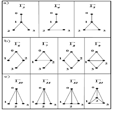
Figure 1: Inequivalent rooted graphs for $N=L=4$; the root vertex $0$ is directly linked with 1 (a), 2 (b) and 3 (c) vertices.

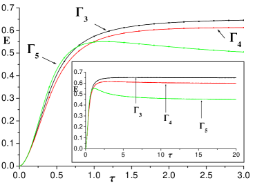
Figure 2: Plot of $E(\tau)$ for the systems $\Gamma_{j}$,$j=3,4,5$.

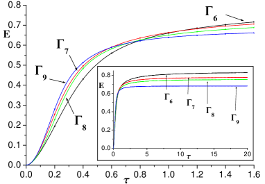
Figure 3: Plot of $E(\tau)$ for the systems $\Gamma_{j}$,$j=6,7,8,9$.

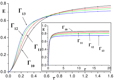
Figure 4: Plot of $E(\tau)$ for the systems $\Gamma_{j}$,$j=10,11,12,13$.

This peculiar behaviour can be somehow understood analytically in the following way. Let us consider for example the system represented by $\Gamma_{5}$; the latter belongs to a class of systems whose Hamiltonian, in the pure tunneling regime ($\varepsilon=0$), can be written as $H=-\tau(b_{0}^{\dagger}b_{1}+{\rm{h.c.}})-\tau\sum_{i\neq j=1}^{L-1}b_{i}^{\dagger}b_{j}.$It corresponds to the topology $\Gamma$ in which the vertex $0$ is connected only with the vertex $1$ whereas the subgraph with vertices $\{1,\ldots,L\}$ is a complete one. Now we provide a simple argument showing that, in the large tunneling amplitude limit and for a large number of vertices, the ground-state entanglement of the vertex $0$ for the systems described by the above Hamiltonian is vanishing.

By introducing the Fourier operators ${\tilde{b}}_{k}:=1/\sqrt{L-1}\sum_{j=1}^{L-1}\exp(\frac{2\pi kj}{L-1})b_{j}\;(k=0,\ldots,L-2)$ the Hamiltonian associated to $\Gamma_{5}$ (with $\varepsilon=0)$ can be rewritten as $H=-\tau(L-1)(H_{0}+H_{1}),$ where $H_{0}={\tilde{b}}_{0}^{\dagger}{\tilde{b}}_{0},\;H_{1}=(L-1)^{-1}[(b_{0}^{\dagger}b_{1}+{\rm{h.c.}})-N_{L-1}],$where $N_{L-1}:=\sum_{j=1}^{L-1}b_{j}^{\dagger}b_{j}.$ The second term in the equation above can be regarded, for $L\mapsto\infty,$ as a small perturbation of the first with coupling constant$\sim L^{-1}.$ It follows that the ground state of $H_{0}$ with $N=L$ particles, for $L=\infty$ is given by a condensate over the mode ${\tilde{b}}_{0},$ i.e., $|\Psi_{GS}\rangle_{L=\infty}\sim({\tilde{b}}_{0}^{\dagger})^{L}|0\rangle.$ In this latter state the mode $0$ clearly factors out with zero occupation number, therefore we have vanishing mode entanglement. A simple first-order pertubation evaluation gives $|\Psi_{GS}\rangle_{L}\sim|\Psi_{GS}\rangle_{L=\infty}-L^{-1}b_{0}^{\dagger}{\tilde{b}}_{0}^{\dagger(L-1)}|0\rangle$ which shows that, for large enough $L,$ the entanglement of the zero mode is a monotonically decreasing function of $L.$ This large $L$ behaviour is anticipated by the system $\Gamma_{5}$: here $L$ is finite and small, therefore $E(\tau)$ does not go to zero but it decreases and it reaches a finite non-zero value in the asymptotic regime i.e., $\tau\gg 1.$ The result presented above is robust against the turning on of a small self-interaction coupling $\varepsilon\neq 0$ Indeed even such a terms would be order $L^{-1}$ with respect $H_{0}$ gen

This discussion indicates that the size of lowest single particle eigenvalue of $\Gamma-\{0\}$ plays a major role in determining the entanglement properties we analyze in this paper. This quantity in turn is well-known to have a clear topological meaning, for example for a regular graph with order $r$ vertices one has $\varepsilon_{0}=-r$ graph . Roughly speaking, the greater the connectivity of $\Gamma-\{0\}$ the greater $|\varepsilon_{0}|.$

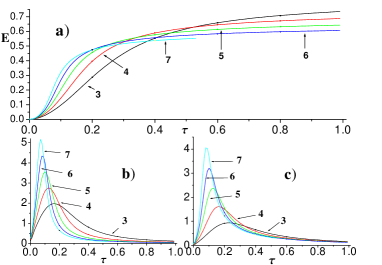
Figure 5: Plot of : a) $E(\tau)$, b) derivative of $E(\tau)$, c) derivative of $\langle n_{i}^{2}\rangle-\langle n_{i}\rangle^{2}$ for the complete graphs with $j=3,4,5,6,7$

Insultator-Superfluid cross-over.– In this section we show that the kind of bi-partite entanglement we analyzed in this paper provides useful insights on the itinerant vs localized character of the particles in the ground state. In particular $E(\tau)$ can be related to the local particle number variance that it is a standard tool to study the insulator-superfluid transition bec_mott . We give a description of the simulation results of for the case of complete graphs. To start with one can consider the simplest possible case, given by $L=2$ i.e., the bosonic dimer hines . It is elementary to see that the ground state of (1) with $\varepsilon=1,$ given then given by $|\Psi_{GS}(\tau)\rangle:=\cos(\theta/2)|11\rangle+\sin(\theta/2)(|02\rangle+|20\rangle)/\sqrt{2},$ where $\theta=-\tan^{-1}(2\tau/\varepsilon)$ from which it follows immediately that the ground-state entanglement is given by $E(\tau)=-\cos^{2}(\theta/2)\ln\cos^{2}(\theta/2)-\sin^{2}(\theta/2)\ln(\sin^{2}(\theta/2)/2).$ It is imeediate to see that $E(\tau)$ is a monotonic increasing function of $\tau;$ maximal entanglement is then achieved in the pure tunneling regime.

In order to measure the itinerant character of the particles over the graph is useful to analyze the ground-state variance of the local occupation numbers i.e., $\langle n_{i}^{2}\rangle-\langle n_{i}\rangle^{2},(i\in V).$ This quantity plays the role of a sort of order parameter in the insulator-superfluid transition: small (large) values of it are associated to an insulator (superfluid). In the dimer case one gets the variance $\sin^{2}(\theta)=1/2(1-1/\sqrt{1+4\tau^{2}})$ that it is again a monotonic increasing function of $\tau$; its derivative shows a peak for $\tau=1/2\sqrt{2}.$ The same kind of qualitative behaviour is displayed by $E(\tau)$ and by its derivative.

We considered complete graphs corresponding an increasing number of sites to i.e., $N=L=3,4,5,6,7$, see figure ($5$). In this case $E(\tau)$, which is plotted in the graphics $a)$, increses monotonically for all the interval $[0,\tau_{max}]$, $\tau_{max}=1$. In the inset of the figure ($5$) it is plotted the variance $\langle n_{i}^{2}\rangle-\langle n_{i}\rangle^{2},(i\in V)$, that, in view of the symmetry of the systems, is the same for all the sites $i$. As for the mode entanglement it increases monotonically for all the interval $[0,\tau_{max}]$. We have therefore plotted the derivative of this quantity and we have compared it with the derivative of the mode entanglement, see graphics $c)$ and $b)$ in figure ($5$). Of course the insulator-superfluid phase transition occurs only in the thermodynamic limit (when $N,L\rightarrow\infty$) so the peak in the derivative plot can only be regarded as a far precursor of this transition. In this case, the derivative exibits the behaviour expected by such a precursor, in fact, as $N=L$ increases it becomes more and more peaked; in presence of an actual phase transition it should display a singular behaviour in correspondance of a critical value $\tau_{c}$ of the tunneling parameter. These results clearly show that $E(\tau)$ has the same qualitative behaviour of the variance the local particle variance comp and therefore, at least for complete graphs, it represents on itself a useful quantity to analyze the cross-over between insulating and super-fluid phases. We observe that this result is reminescent of an analog one for the metal-insulator transition in the Fermionic Hubbard nodel you1 .

Conclusions.– We have analyzed ground-state entanglement of interacting bosons for all the four vertices graphs. The ground-states for all possible graph topologies have been obtained by numerical diagonalization and the entanglement of one vertex with respect to all the others has been computed as a function of the tunneling amplitude. This analysis allows to order graphs, for a given tunneling amplitude $\tau,$ in terms of the amount of this bi-partite ground-state entanglement $E(\tau).$ Remarkably this order actually depends on both $\tau$ and the graph topology: for small (large) $\tau$ the higher (lower) the modulus of the minimum single-particle eigenvalue of the graph $\Gamma$ (sub-graph $\Gamma-\{0\}$) the higher (lower) the mode entanglement. Moreover numerical results show un unexpected, non monotonic, behaviour of $E(\tau)$ for some particular graph topologies. Such a phenomenon can be understood analytically in the limit of no self-interaction. We finally showed, for complete graphs of different sizes, that $E(\tau)$ contains useful information about the cross-over between the insulator and superfuild regime. The analysis of the role of topology and self-interaction on multi-partite entaglement, for example by considering all possible bi-partitions of the graph at once, is a more demanding task clearly deserving future investigations

P.Z. gratefully acknowledges financial support by Cambridge-MIT Institute Limited and by the European Union project TOPQIP (Contract IST-2001-39215)

References

- (1) M. Horodecki, P. Horodecki and R. Horodecki, in “Quantum Information - Basic Concepts and Experiments”, Eds. G. Alber and M. Weiner, in print (Springer, Berlin, 2000).
- (2) See, e.g., D.P. DiVincenzo and C. Bennet, Nature 404, 247 (2000) and references therein.
- (3) A. Osterloh, L. Amico, G. Falci, and R. Fazio, Nature 416, 608 (2002); T.J. Osborne and M.A. Nielsen, Phys. Rev. A 66, 032110 (2002; G. Vidal, J. I. Latorre, E. Rico, and A. Kitaev Phys. Rev. Lett. 90, 227902 (2003) J. I. Latorre, E. Rico, G. Vidal quant-ph/0304098; X. Wang, H. Li, B. Hu quant-ph/0308118; S. Gu, H. Lin, Y. Li quant-ph/0307131; S. Gu, Y. Li, H. Lin quant-ph/0310030
- (4) Chris D. Godsil, Gordon F. Royle, Algebraic Graph Theory, Graduate Texts in Mathematics, Springer Verlag (2001)
- (5) M. P. A. Fisher et al., Phys. Rev. B 40, 546 (1989).
- (6) P. Zanardi, Phys. Rev. A 67, 054301 (2003
- (7) P. Zanardi, Ch. Zalka, L. Faoro. Phys. Rev. A 62 (2000) 030301(R)
- (8) A. Hamma, P. Zanardi quant-ph/0308131
- (9) P. Giorda, P. Zanardi, quant-ph/0304151
- (10) P. Zanardi, Phys. Rev. A65, 042101 (2002); P. Zanardi, X-G. Wang, J. Phys. A:Math. Gen., 35, 7947 (2002)
- (11) J. R. Gittings and A. J. Fisher, Phys. Rev. A 66, 032305 (2002)
- (12) S. van Enk,Phys. Rev. A67, 022303 (2003)
- (13) Y. Shi, Phys. Rev. A67, 024301 (2003)
- (14) J. Schliemann, D. Loss, and A. H. MacDonald, Phys. Rev. B 63, 085311 (2001); J. Schliemann, J. I. Cirac, M. Kus, M. Lewenstein, and D. Loss, Phys. Rev. A 64, 022303 (2001).
- (15) R. Paskauskas, L. You, Phys. Rev. A64, 043210 (2001)
- (16) Y. S. Li, B. Zeng, X. S. Liu and G. L. Long, Phys. Rev. A64, 054302 (2001)
- (17) H. M. Wiseman and J. A. Vaccaro Phys. Rev. Lett. 91, 097902 (2003)
- (18) P. Zanardi, Phys. Rev. Lett. 87, 077901 (2001); P. Zanardi, D. Lidar, and S. Lloyd, quant-ph/0308043.
- (19) N. Schuch, F. Verstraete, I Cirac quant-ph/0310124
- (20) D. Jaksch et al., Phys. Rev. Lett. 81, 3108 (1998).
- (21) G. J. Milburn et al., Phys. Rev. A55, 4318 (1997);
- (22) Z.B. Chen and Y.D. Zhang, Phys. Rev. A 65, 022318 (2002)
- (23) R. Ionicioiu and P. Zanardi, Phys. Rev. A66, 050301 (2002)
- (24) L.-M. Duan, J. I. Cirac, and P. Zoller, Phys. Rev. A65, 033619 (2002)
- (25) C. Simon, Phys. Rev. A 66, 052323 (2002)
- (26) A. P. Hines et al. , Phys. Rev. A67, 013609 (2003).
- (27) A. Micheli, D. Jaksch, J. I. Cirac, and P. Zoller, Phys. Rev. A67, 013607 (2003)
- (28) L. You, Phys. Rev. Lett. 90, 030402 (2003)
- (29) L.-M. Duan, E. Demler, M. D. Lukin, cond-mat/0210564
- (30) M. Greiner et al., Nature 415, 39 (2002).
- (31) We can further generalize the above argument as follows. The Hamiltonian (1) can be written, for as a sum of two terms and the first containing all the contributions involving the mode and the second describing just the sub-graph Let the diagonal form of If we define as the single-body ground state, the ground-state of with particle is a a condensate over the corresponding eigen-mode with zero particle in the vertex. One can write where is a sum over the excited single-body terms of By denoting with the number of edges linking the vertex with the rest of the graph, the second term in the equation above is at most of the order When the modulus of this ratio gets very small e.g., and for large the contribution is a perturbative one and at zero temperature all the particles tend to be localized within the sub-graph i.e., no entanglement of the vertex with the others.
- (32) This can be understood by observing that the reduced density matrix is a diagonal i.e., and is just the (normalized) Shannon entropy of the probability distribution whereas the local particle number variance is
- (33) S. -J. Gu, Y. -Q. Li, H. -Q. Lin quant-ph/0310030