Cavity Assisted Nondestructive Laser Cooling of Atomic Qubits

Abstract

We analyze two configurations for laser cooling of neutral atoms whose internal states store qubits. The atoms are trapped in an optical lattice which is placed inside a cavity. We show that the coupling of the atoms to the damped cavity mode can provide a mechanism which leads to cooling of the motion without destroying the quantum information.

1 Introduction

Quantum optical schemes for quantum information processing employ long lived internal (spin or hyperfine) states of atoms or ions to store the qubit [1]. In many of the proposals for scalable quantum computing these qubits are stored in a storage area, and must be moved together to perform e.g. a two-qubit gate operation entangling the atoms [2, 3]. Moving atoms will typically cause heating, and thus the question arises to what extent the motion of the qubit atoms can be cooled nondestructively, i.e. without affecting the coherence of the qubit. In the case of quantum computing with trapped ions this is achieved by sympathetic cooling [4]: the “qubit ion” is coupled via the Coulomb force to a second “cooling ion” (of a different species), which is laser cooled [5, 6]. This cooling is nondestructive because the Coulomb force is identical for the two qubit states $|0\rangle$, $|1\rangle$. Quantum computing with neutral atoms can be performed by storing atoms in optical lattices generated by counterpropagating laser beams. By moving the atoms in a spin dependent optical lattice [7, 8] one can induce controlled collisions between the qubits leading to multi particle entanglement [7, 9, 10]. One possibility for nondestructive cooling in an optical lattice is sympathetic collisional cooling by immersion of the qubit atoms stored in the lattice in an atomic Bose Einstein condensate [11]. Of course, laser cooling of qubit atoms stored in the wells of an optical lattice potential cannot be directly applied, as the optical pumping associated with the laser cooling process destroys the coherence. Instead we will investigate below a scenario of nondestructive laser cooling of atomic qubits in moving optical lattice potentials which is achieved by coupling to a (low-$Q$) optical cavity. These results are also of interest for implementations of quantum computation and quantum communication with optical cavities [12, 13, 14, 15, 16].

Cavity assisted laser cooling is a well-studied process [17, 18, 19, 20, 21, 22, 23], both theoretically and experimentally. In the present paper we will elaborate on two distinguishing features which make cavity assisted laser cooling of interest for quantum computing with atoms in optical lattices. We will study a scenario where a set of qubit atoms is stored in individual wells of an optical lattice potential. By moving the lattice we will heat the atom motion. However, to the extent the optical lattice potentials seen by the two qubit states are identical, this transport will not destroy the coherence of the internal atomic states. Cavity assisted recooling of the motional degrees works by converting phonons to cavity photons in a coherent laser assisted process. These cavity photons dissipate through the cavity mirror. With an appropriate choice of internal qubit states, this cooling process does not distinguish between the two qubits, and is thus nondestructive. We also note that moving $N$ qubits in an accelerating lattice will excite the collective center of mass mode of these atoms. This is precisely the mode which is cooled most efficiently by our cavity cooling scheme. The scheme we investigate is, in principle, capable to achieve ground state cooling in the optical wells, although in practice nondestructive cooling to the Lamb-Dicke regime, where the atom is localized in a region much smaller than the optical wave length, may be sufficient.

The paper is organized as follows. In Sec. 2 we present two different specific setups and we calculate the equations of motion in both cases for a single qubit and for the center of mass motion of N qubits. In Sec. 3 we derive analytical expressions for the steady state temperature $T_{f}$ and the cooling time $\tau$ of the atoms and compare them with numerical calculations. Finally, in Sec. 4 we discuss possible imperfections of the system.

2 The Model

In this section we introduce two different setups for cooling the motion of neutral atoms without destroying the quantum information stored in two long lived degenerate internal ground states $\left|g_{1}\right\rangle\equiv\left|0\right\rangle$ and $\left|g_{2}\right\rangle\equiv\left|1\right\rangle$. In the first setup the atoms are trapped and cooled by the field of a ring cavity while in the second case trapping is achieved by an optical lattice and the cavity is solely used for cooling the atoms. To be specific, we will choose the two qubit states to be two Zeeman states, e.g. $|J=1/2,M=\pm 1/2\rangle$, and we will assume identical (symmetric) coupling of these states to the laser and the cavity mode to achieve cooling which does not distinguish between the two qubit states. Our goal is to derive cooling equations first for a single qubit, and then for the center of mass motion of $N$ qubits.

2.1 Optical Lattice in a Ring Cavity

We consider neutral atoms in a ring cavity as shown in Fig. 1a). Two coherent fields $\beta_{R}$ and $\beta_{L}$ drive two counter-propagating running waves adding up to a standing wave inside the cavity. We first consider a single qubit in this ring cavity and then extend the system to $N$ qubits.

2.1.1 Single Qubit

In a frame rotating with the laser frequency $\omega_{L}$, the Hamiltonian describing the cavity fields and one atom is given by

$$H=H_{\rm A}+H_{\rm C}+H_{\rm AC}+H_{\rm F}+H_{\rm CF}+H_{\rm bath}+H_{\rm sys-bath}$$ (1)

with ($\hbar=1$)

$$H_{\rm A}=\frac{p^{2}}{2m}+(-\Delta)\left(\left|e_{1}\right\rangle\left\langle e_{1}\right|+\left|e_{2}\right\rangle\left\langle e_{2}\right|\right),$$ (2)

$$H_{\rm C}=(-\Delta_{c})(a_{R}^{\dagger}a_{R}+a_{L}^{\dagger}a_{L}),$$

$$H_{\rm AC}=g\left[\left(a_{R}\rme^{\rmi(kx-\omega_{L}t)}+a_{L}\rme^{-\rmi(kx+\omega_{L}t)}\right)\left(\sigma_{1}^{+}+\sigma_{2}^{+}\right)+{\rm h.c.}\right],$$

$$H_{\rm F}=\sum_{j=R,L}\int{\rm d}\omega\omega b_{\omega,j}^{\dagger}b_{\omega,j},$$

$$H_{\rm CF}=\rmi\sqrt{\kappa}\sum_{j=R,L}\int{\rm d}\omega\left(a_{j}^{\dagger}b_{\omega,j}\rme^{\rmi\omega_{L}t}-{\rm h.c.}\right).$$

Here the detuning of the laser from the atomic transition frequency $\omega_{\rm eg}$ is given by $\Delta=\omega_{L}-\omega_{\rm eg}$ and the detuning from the cavity frequency $\omega_{c}$ by $\Delta_{c}=\omega_{L}-\omega_{c}$. Furthermore, $H_{\rm A}$ gives the kinetic and the internal energy of the atom, respectively, where $p$ is the momentum operator and $m$ is the mass of the atom. The two long lived degenerate ground states carrying the qubit are $\left|g_{1}\right\rangle\equiv\left|0\right\rangle$ and $\left|g_{2}\right\rangle\equiv\left|1\right\rangle$, as sketched in Fig. 1 and we assume the atom to have two degenerate excited states $\left|e_{1}\right\rangle$ and $\left|e_{2}\right\rangle$. The Hamiltonian $H_{\rm C}$ describes a ring cavity with a clockwise and counter-clockwise propagating mode, and bosonic destruction (creation) operators $a_{R(L)}$ ($a^{\dagger}_{R(L)}$). In dipole and rotating wave approximation, the interaction of the atom with the cavity field has the form $H_{\rm AC}$, where $\sigma^{+}_{1}=\left|e_{1}\right\rangle\left\langle g_{1}\right|$, $\sigma^{+}_{2}=\left|e_{2}\right\rangle\left\langle g_{2}\right|$ and $\sigma^{-}_{j}=(\sigma^{+}_{j})^{\dagger}$, $j=1,2$. Furthermore, $g$ denotes the single photon Rabi frequency, and $k$ is the wave vector of the laser light. The free Hamiltonian for the external driving field is denoted by $H_{\rm F}$ and $H_{\rm CF}$ describes the interaction of this field with the two cavity modes, where $\kappa$ is the photon loss rate through the cavity mirrors. The bosonic annihilation (creation) operators for the field in the mode $\omega$, $b_{\omega,R(L)}$ ($b_{\omega,R(L)}^{\dagger}$) fulfill the commutation relations $[b_{\omega,R(L)},b_{\omega^{\prime},R(L)}^{\dagger}]=\delta(\omega-\omega^{\prime})$. Finally, the term $H_{\rm sys-bath}$ describes the interaction of the atom with a photonic bath $H_{\rm bath}$, which leads to spontaneous emission. These terms are of standard form and can be found e.g. in [24, 25].

We assume the electric field driving the two cavity modes to be coherent, representing a classical field with amplitudes $\beta_{\rm in,R(L)}(t)$. As described in detail in A we go to a picture where the incident driving field explicitly enters the Hamiltonian. This results in a vacuum input state for the cavity and the additional driving term

$$\widetilde{H}_{\rm CF}=\rmi\sqrt{2\kappa}\left(\beta_{\rm in}(t)A_{+}^{\dagger}-A_{+}\beta_{\rm in}(t)^{*}\right)$$ (3)

in the Hamiltonian. Here we have defined $A_{\pm}=\left(a_{R}\pm a_{L}\right)/\sqrt{2}$, and furthermore assumed symmetric driving $\beta_{{\rm in},R}(t)=\beta_{{\rm in},L}(t)\equiv\beta_{\rm in}(t)$.

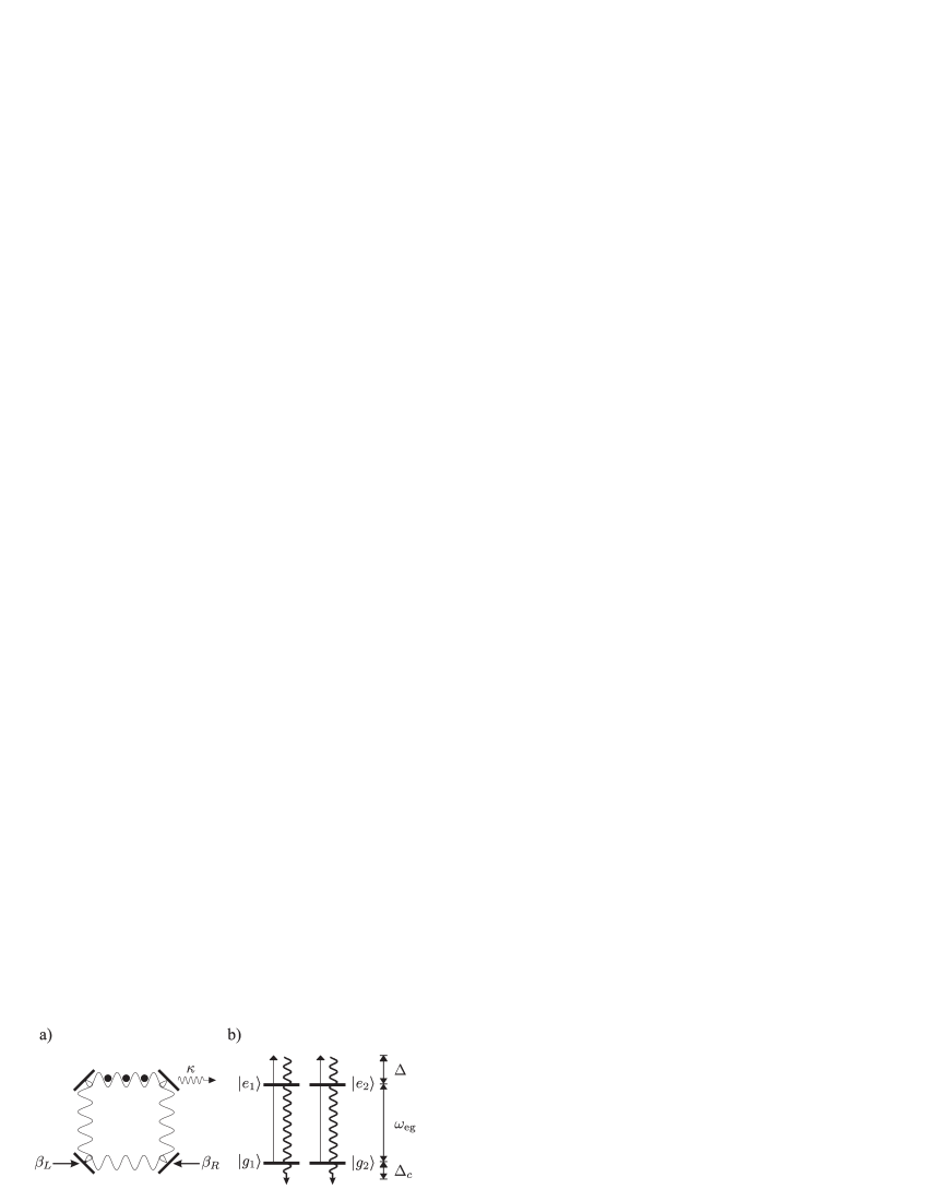
Figure 1: a) Experimental setup as described in the text. b) Schematic picture of the internal level structure, the involved frequencies and detunings. The ground state $\left|g_{1}\right\rangle$ $(\left|g_{2}\right\rangle)$ is identified with the qubit state $\left|0\right\rangle$ $(\left|1\right\rangle)$. As a concrete example one can chose the fine structure states (e.g. of Na or Rb) as shown in Fig. 7.

The dynamics of the system thus obeys a master equation (see e.g. [24])

$$\dot{\rho}=-\rmi\left[H_{{\rm sys}},\rho\right]+\mathcal{L}(\rho),$$ (4)

where the Hamiltonian of the system is given by $H_{\rm sys}=H_{\rm A}+H_{\rm C}+H_{\rm AC}+\widetilde{H}_{\rm CF}$. The Liouville superoperator $\mathcal{L}$ has the form

$$\mathcal{L}(\rho) = \frac{\kappa}{2}\sum_{i=\pm}\left(2A_{i}\rho A^{\dagger}_{i}-A^{\dagger}_{i}A_{i}\rho-\rho A^{\dagger}_{i}A_{i}\right)$$ (6)

$$+\frac{\gamma}{2}\sum_{i=\pm}\left(2\sigma^{-}_{i}\rho\sigma^{+}_{i}-\sigma^{+}_{i}\sigma^{-}_{i}\rho-\rho\sigma^{+}_{i}\sigma^{-}_{i}\right).$$

The first line Eq. (6) describes loss due to the imperfectness of the cavity mirrors, and the second line Eq. (6) is due to the spontaneous emission of the atom with emission rate $\gamma$. Note that based on the choice of atomic states and laser and cavity polarizations, the laser and cavity couplings as well as the spontaneous emission rates are assumed to be identical for the two qubit states.

Next we decompose the cavity mode operators $A_{\pm}$ into a $\mathbbm{C}$-number $\alpha_{\pm}=\langle A_{\pm}\rangle$ describing the coherent part and an operator part $\delta\!A_{\pm}=A-\alpha$ describing the fluctuations. The mean values $\left\langle A_{\pm}\right\rangle=\alpha_{\pm}$ are calculated in the steady state. From Eq. (4) the respective equations of motion for $\left\langle A_{\pm}\right\rangle$ can be easily obtained, yielding

$$\frac{\rmd}{\rmd t}{\left\langle A_{+}\right\rangle}=(\rmi\Delta_{c}-\frac{\kappa}{2})\left\langle A_{+}\right\rangle+\sqrt{2\kappa}\beta_{\rm in},$$

$$\frac{\rmd}{\rmd t}{\left\langle A_{-}\right\rangle}=(\rmi\Delta_{c}-\frac{\kappa}{2})\left\langle A_{-}\right\rangle.$$ (7)

From the steady state solution of Eqs. (2.1.1) we find

$$\alpha_{+}=\frac{\sqrt{2\kappa}\beta_{\rm in}}{-\rmi\Delta_{c}+\frac{\kappa}{2}}\equiv\alpha,\qquad\alpha_{-}=0.$$ (8)

Applying this transformation to the system Hamiltonian we find $H_{\rm sys}=H_{\rm A}+H_{\rm C}+\tilde{H}_{\rm int}$, where in $H_{\rm C}$ the operators $A_{\pm}$ are replaced by $\delta\!A_{\pm}$ and $\tilde{H}_{\rm int}$ is given by

$$\tilde{H}_{\rm int}=\sqrt{2}g\left[\left((\delta A_{+}+\alpha)\cos{kx}+\rmi\delta\!A_{-}\sin{kx}\right)\left(\sigma^{+}_{1}+\sigma^{+}_{2}\right)\right.$$

$$\left.\qquad+{\rm h.c.}\right].$$

The Liouville operator $\mathcal{L}$ reduces to

$$\mathcal{L}(\rho) = \frac{\kappa}{2}\sum_{i=\pm}\left(2\delta\!A_{i}\rho\delta\!A^{\dagger}_{i}-\delta\!A^{\dagger}_{i}\delta\!A_{i}\rho-\rho\delta\!A^{\dagger}_{i}\delta\!A_{i}\right),$$ (9)

where we have assumed large detunings $\Delta$ and consequently neglected the spontanous emission, as it is suppressed by a factor $\propto g^{2}/\Delta^{2}$. Furthermore, in this approximation we can adiabatically eliminate the excited states $\left|e_{1}\right\rangle$ and $\left|e_{2}\right\rangle$ and obtain

$$H_{{\rm eff}} =\mathbbm{1}_{i}\otimes\left(\frac{p^{2}}{2m}-\Delta_{c}\left(\delta\!A^{\dagger}_{+}\delta\!A_{+}+\delta\!A^{\dagger}_{-}\delta\!A_{-}\right)\right.$$

$$\left.+\frac{2g^{2}}{\Delta}\left(\alpha^{2}\cos^{2}kx+\rm i\alpha(\delta\!A^{\dagger}_{-}-\delta\!A_{-})\cos{kx}\sin{kx}+\delta\!A^{\dagger}_{-}\delta\!A_{-}\sin^{2}kx\right)\right),$$

where we have only kept the leading terms in $\delta\!A$, assuming small fluctuations $|\left\langle\delta A\right\rangle|\ll|\alpha|$. In Eq. (2.1.1) the operator $\mathbbm{1}_{i}=\left|g_{1}\right\rangle\left\langle g_{1}\right|+\left|g_{2}\right\rangle\left\langle g_{2}\right|$ which we do not write explicitly in the following. Thus, due to our choice of symmetric coupling and dissipation, the information encoded in the qubit (i.e. the amplitudes of the two internal ground states) is not affected by the time evolution Eq. (4). Furthermore, the operators $\delta\!A_{+}$ and $\delta\!A^{\dagger}_{+}$ do not couple to any other degrees of freedom of the system and, therefore, we drop them in the following.

The periodic optical lattice inside the cavity is given by the term $V_{0}\cos^{2}{kx}$ in Eq. (2.1.1) with a depth of $V_{0}=2g^{2}\alpha^{2}/|\Delta|$. For a blue (red) detuned lattice and a kinetic energy of the atom much smaller than the depth of the optical lattice (i.e. $\left\langle p^{2}\right\rangle/2m\ll V_{0}$), the atoms are trapped near the (anti)nodes of the standing wave. Thus, we can approximate each well of the lattice by a harmonic oscillator with frequency $\nu=2g\alpha k/\sqrt{m\Delta}$. In this approximation $\mathcal{L}$ is given by

$$\mathcal{L}(\rho)=\frac{\kappa}{2}\left(2a\rho a^{\dagger}-a^{\dagger}a\rho-\rho a^{\dagger}a\right),$$ (11)

where we have introduced $a\equiv\delta\!A_{-}$ and the system Hamiltonian reduces to

$$H_{\rm sys}=\nu c^{\dagger}c+\nu_{c}a^{\dagger}a+\rmi g_{{\rm eff}}\left(c+c^{\dagger}\right)\left(a^{\dagger}-a\right).$$ (12)

The bosonic creation (annihilation) operator $c^{\dagger}$ ($c$) describes the quantized motion of the atom in a harmonic potential of frequency $\nu$ coupled to the cavity mode $a$ with the effective coupling strength $g_{{\rm eff}}=\nu/2\alpha\eta$, as shown in Fig. 2. In Eq. (12) we also used the definitions $\nu_{c}=-\Delta_{c}+\frac{2g^{2}}{\Delta}$ for the frequency of the cavity mode $a$, and $\eta=\sqrt{k^{2}/2m\nu}$ the Lamb-Dicke parameter. The shift $2g^{2}/\Delta$ can be interpreted as a refractive index due to the back-action of the atom on the cavity field. In the limit $g/\nu\ll 1,\nu=\nu_{c}$ we can apply the rotating wave approximation (RWA) to Eq. (12), and find

$$H_{\rm RWA}=\nu c^{\dagger}c+\nu_{c}a^{\dagger}a+\rmi g_{{\rm eff}}\left(ca^{\dagger}-ac^{\dagger}\right).$$ (13)

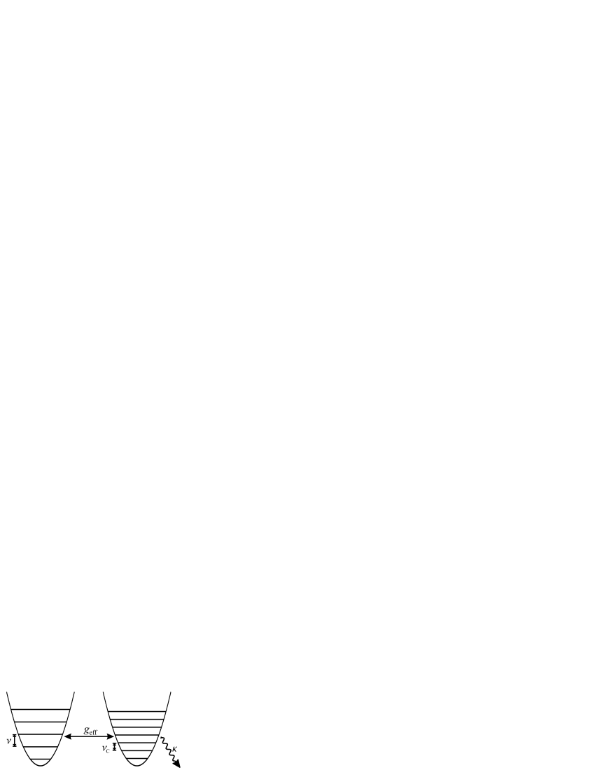
Figure 2: The two coupled harmonic oscillators corresponding to the atomic motion and the cavity with frequencies $\nu$ and $\nu_{c}$, respectively. The coupling strength is denoted by $g_{\rm eff}$ and $\kappa$ is the photon loss rate through the cavity mirrors.

We finally turn to the physical interpretation of our results. The coupled oscillator Hamiltonian Eq. (12) describes the coherent transfer of phonons (vibrational excitations) to cavity photons. Due to its high frequency, the optical cavity mode is coupled to an effective zero temperature heat bath. Cavity phonons will decay through the mirror according to Eq. (11), dissipating the energy.

A physically equivalent picture can be given in terms of a dissipative optical lattice according to Eq. (2.1.1). In the ring cavity we have two counterpropagating modes, which we rewrite as $\cos kx$ (+) and $\sin kx$ (-) standing wave modes. By driving the cavity symmetrically from the outside with two lasers, the standing wave $\cos kx$ will have a large occupation of phonons $|\alpha|^{2}$, giving rise to an optical lattice potential, while the not-driven $\sin kx$ mode will be in a vacuum state. Motion of an atom in the optical lattice will redistribute the photons among the two modes. In particular, atomic motion will transfer photons to the (initially empty) $\sin kx$ mode, i.e. the optical lattice potential will be slightly shifted by atomic motion. On the other hand, the photons occupying the $\sin kx$ mode can decay through the cavity mirror, giving rise to a damping. Thus we have the picture, where the atomic motion in the optical wells acts back on the lattice to produce a (small amplitude) displacement of the lattice. These oscillations of the optical lattice will damp to their equilibrium position by the cavity decay, thus cooling the motion of the atom. With an appropriate choice of qubit states we assure that the dissipative optical lattice potential seen by the two qubit states are identical. This ensures that the cooling does not destroy the coherence of the qubit.

Finally, we note that our laser cooling model maps on to a remarkably simple mathematical model of coupled harmonic oscillators with linear damping. Thus we find a straightforward solution in terms of Gaussian states of the two modes. Below we will extend the model to $N$ qubits, and then to the case of a time dependent moving lattice to illustrate the cooling dynamics.

2.1.2 N Qubits

The derivation of the $N$-particle Hamiltonian is similar to the calculations presented in Sec. 2.1.1 and leads to

$$H=\nu\sum_{\mu=1}^{N}c_{\mu}^{\dagger}c_{\mu}+\nu_{c}(N)a^{\dagger}a+\rmi g_{\rm eff}\sum_{\mu=1}^{N}\left(c_{\mu}+c_{\mu}^{\dagger}\right)\left(a^{\dagger}-a\right),$$ (14)

where the index $\mu$ labels the particles. All parameters apart from $\nu_{c}(N)=-\Delta_{c}+2g^{2}N/\Delta$ and the refractive index now given by $2g^{2}N/\Delta$ remain unchanged. In Eq. (14) we have assumed the effective coupling constant to be the same for each particle ($g_{\rm eff,\mu}=g_{\rm eff}$). The Hamiltonian Eq. (14) describes N harmonic oscillators corresponding to the quantized motion of the atoms coupled to the single cavity mode $a$. The coupling term in Eq. (14) has exactly the same form as in the single qubit case Eq. (12) if we define the center of mass (COM) annihilation (creation) operator $C$ ($C^{\dagger}$) given by $C=1/\sqrt{N}\sum_{\mu}c_{\mu}$ and introduce the coupling constant $\tilde{g}=\sqrt{N}g_{\rm eff}$. The resulting form of Eq. (14) already indicates that only the collective mode $C$ will be cooled in our approximative description. We note that previous publications [26, 27] have already shown in a semiclassical approximation, that also the (N-1) relative vibrational modes can be cooled with our setup, but on a much larger timescale.

As will be discussed in detail below, transport of $N$ atoms in an accelerating lattice leads to coherent oscillations of the center-of-mass mode of all the atoms. Our cooling scheme cools this particular collective mode with high efficiency due to the collective enhancement $g_{\rm eff}\rightarrow g_{\rm eff}\sqrt{N}$ of the phonon-photon.

2.2 Optical Lattice in a Standing Wave Cavity

As a possibly more convenient setup, we replace the ring cavity of Sec. 2.1 by a standing wave cavity providing the cooling. We assume the optical lattice holding to the atoms to be produced by two counter-propagating laser beams, which we shine into the resonator at a small angle, as shown in Fig. 3, whereas in the previous system the driving field entered the cavity through the cavity mirrors.

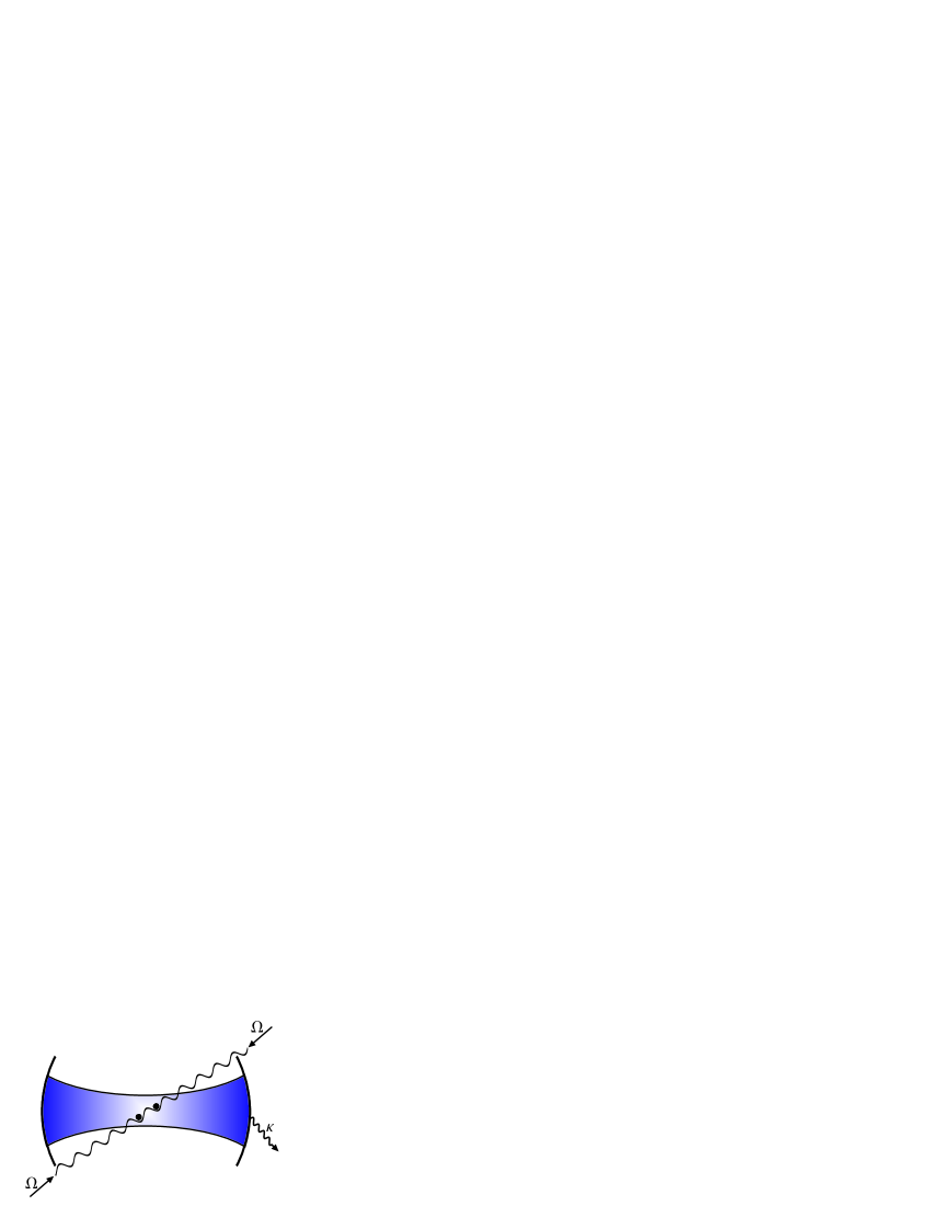
Figure 3: Schematic experimental setup as described in the text.

The total Hamiltonian takes on the form $H=H_{\rm A}+H_{\rm C}+H_{\rm AC}+H_{\rm AL}$, where

$$H_{\rm A}=\frac{p^{2}}{2m}+(-\Delta)(\left|e_{1}\right\rangle\left\langle e_{1}\right|+\left|e_{2}\right\rangle\left\langle e_{2}\right|),$$ (15)

$$H_{\rm C}=(-\Delta_{c})a^{\dagger}a,$$

$$H_{\rm AL}=\frac{\Omega}{2}\rmi\sin{kx}\left(\sigma^{+}-\sigma^{-}\right),$$

$$H_{\rm AC}=g\cos{k_{c}x}\left(a\sigma^{+}+a^{\dagger}\sigma^{-}\right),$$

and $\sigma^{\pm}=(\sigma_{1}^{\pm}+\sigma_{2}^{\pm})$. The Hamiltonians $H_{\rm A}$ and $H_{\rm C}$ denote the energy of the atom and the cavity with bosonic creation and annihilation operators $a^{\dagger}$ and $a$, respectively. The interaction of the laser with Rabi frequency $\Omega$ and the atom is denoted by $H_{\rm AL}$ and $H_{\rm AC}$ describes the atom-cavity coupling ($g$ again denotes the single photon Rabi frequency).

Applying the same approximations as in Sec. 2.1 we find an identical model with the replacements $\nu\rightarrow\tilde{\nu}=\Omega^{2}\eta^{2}/\Delta$ and $\nu_{c}\rightarrow\tilde{\nu}_{c}=-\Delta_{c}+g^{2}/\Delta$, as well as the effective coupling $g_{{\rm eff}}\rightarrow\tilde{g}_{{\rm eff}}=g\Omega\eta/2\Delta$ in Eq. (4). The Lamb-Dicke parameter $\eta$ is $\eta=\sqrt{k/2m\nu}\sim\sqrt{k_{c}/2m\nu}$, where $k_{c}$ and $k$ denote the wave vectors of the cavity and the laser light, respectively. A straightforward extension to $N$ qubits results again in a Hamiltonian of the form (14).

The physical interpretation of this setup is very similar to the previous one with the only difference that the optical lattice is formed by two additional lasers instead of the cavity itself. In this case the motion of the atoms transfers photons from the laser field into the (initially empty) cavity. As in the previous setup the decay of the cavity photons through the cavity mirrors leads to cooling of the atomic motion without affecting the qubit state.

2.2.1 Accelerated optical lattice

Finally, we generalize the model to an accelerated optical lattice. In the setup of Fig. 3 the lattice can easily be moved by introducing a time dependent relative phase $\phi(t)$ between the two counter-propagating laser beams [7, 8]. We find a system Hamiltonian

$$H =\nu c^{\dagger}c+\nu_{c}a^{\dagger}a-\frac{\nu\alpha}{2}\left(c+c^{\dagger}\right)-\rmi g\alpha\cos{(\phi(t))}\left(a^{\dagger}-a\right)$$ (16)

$$+\rmi g\cos{(\phi(t))}\left(c+c^{\dagger}\right)\left(a^{\dagger}-a\right)+\frac{\nu^{2}}{4}\alpha^{2},$$

with $\nu_{c}=-\Delta_{c}+g^{2}\cos^{2}{(\phi)}/\Delta$, $\alpha=\phi/\eta$. The values for $\nu$, $g$ and $\eta$ are defined as above.

3 Results

Below we solve the cooling equations Eq. (4). In Sec. 3.1 we derive analytical expressions for the atomic steady state temperature $T_{f}$ and the cooling time $\tau$. In Sec. 3.2 we show examples for the numerical solution of Eq. (4) in the case of a static lattice as well as for an accelerated lattice.

3.1 Analytical Calculations

The master equation (4) consists of a quadratic system Hamiltonian and a linear damping term. Thus, the Heisenberg equations for the expectation values of the second order moments can be found easily (see B, Eq. (28)). From these we calculate the atomic steady state temperature $T_{F}$

$$k_{B}T_{f}\equiv E_{0}=\nu\left\langle c^{\dagger}c\right\rangle_{\rm SS}=$$ (17)

$$=\frac{g_{\rm eff}^{2}}{2\nu}+\frac{\kappa^{2}+4(\nu-\nu_{c})^{2}}{16\nu_{c}}+\frac{8g_{\rm eff}^{4}\nu_{c}}{\nu\left[\kappa^{2}\nu+4\nu_{c}(-4g_{\rm eff}^{2}+\nu\nu_{c})\right]},$$

with $k_{B}$ the Boltzmann constant and $E_{0}$ the steady state energy. We note that the system is always cooled to the ground state in the limit $g_{\rm eff}\ll\nu\sim\nu_{c}$ (i.e. where the RWA Eq. (13) is valid).

The atomic energy $E_{\rm atom}(t)=\nu\left\langle c^{\dagger}c\right\rangle_{t}$ can be written in the form

$$E_{\rm atom}(t)=\sum_{k}c_{k}\rm e^{\lambda_{k}t}+E_{0},$$ (18)

where the $\lambda_{k}$ are eigenvalues (all having negative real parts) obtained from the equations of motion and the coefficients $c_{k}$ are found from the initial motional state of the atom. If one term dominates in the sum Eq. (18) then $1/|{\rm Re}\lambda_{k}|$ with the corresponding eigenvalue $\lambda_{k}$ gives the cooling time $\tau$. In general, however, the cooling time will be determined by the eigenvalue $\lambda_{k}$ with the largest real part unless the corresponding coefficient $c_{k}$ vanishes. We therefore find an upper bound for the cooling time $\tau$ by

$$\tau=\frac{1}{{\rm min}\{|{\rm Re}\lambda_{k}|\}}_{k}.$$ (19)

In RWA we can easily calculate the eigenvalues $\lambda_{k}$ from the equations of motion given in B, Eq. (29) and find simple analytic estimate for the cooling time $\tau$ in two interesting limits. In the ”Doppler limit”, i.e. $g_{\rm eff}\ll\nu\ll\kappa$, $\nu_{c}=\frac{\kappa}{2}$ we find $\tau\approx\kappa/4g_{\rm eff}^{2}$ and $k_{B}T_{f}\approx\frac{\kappa}{4}$, in close analogy to free space Doppler cooling (see e.g. [28]). In the ”sideband limit”, i.e. $g_{\rm eff}\sim\kappa\ll\nu\sim\nu_{c}$, we obtain $\tau\approx\frac{2}{\kappa}$ and $k_{B}T_{f}\approx g_{\rm eff}^{2}/2\nu$. In the numerical examples in Sec. 3.2 one can see that those analytical expressions are in very good agreement with the exact numerical calculations. These results for the single qubit case can be directly applied to the COM motion of $N$ qubits by replacing $g\rightarrow\tilde{g}$.

3.2 Numerical Results

In this section we show the numerical solution of Eq. (4) for different parameter regimes in the case of a static lattice as well as for an accelerated lattice.

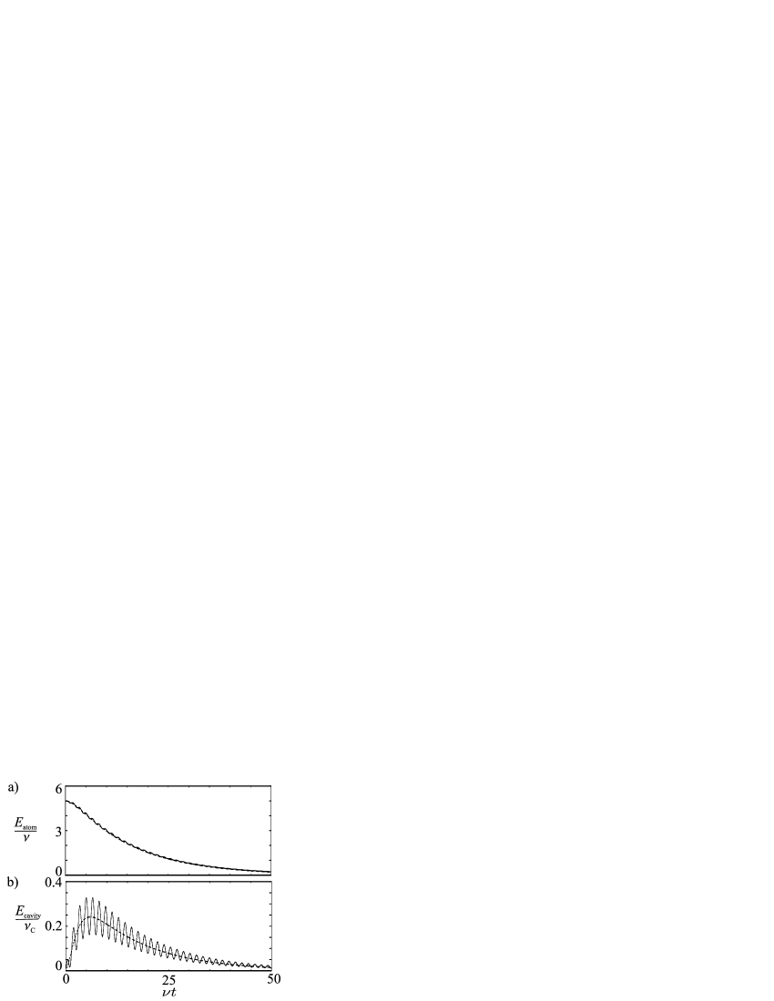
Figure 4: a) Energy of the atomic motion $E_{\rm atom}$ and b) energy of the cavity mode $E_{\rm cavity}$ as a function of time $\nu t$. The parameters are chosen $\kappa=1$, $\nu=\nu_{c}=2$ and $g_{\rm eff}=1/8$. The dashed lines show the time evolution with the effective Hamiltonian $H_{\rm eff}$ in RWA, the solid lines are without the RWA.

Fig. 4 shows the time evolution of the atomic energy $E_{\rm atom}(t)$ and the energy of the cavity mode $a$, $E_{\rm cavity}=\nu_{c}\left\langle a^{\dagger}a\right\rangle_{t}$, as a function of time $\nu t$. Initially the system is assumed to be in a product state with the cavity mode $a$ in its ground state and the mode for the atomic motion in a coherent state. The time evolution of the two energies shows that energy is transferred from the mode $c$ for the atomic motion into the cavity mode. The energy of the cavity mode decreases due to the photon loss through the cavity mirrors, which leads to a cooling of the atomic motion as well. Furthermore Fig. 4 shows a comparison between the time evolution in RWA and without RWA. We can see, that in the RWA no oscillations of the energies occur, i.e. in this approximation the energy is transferred smoothly from one mode into the other and dissipates at a rate $\kappa$.

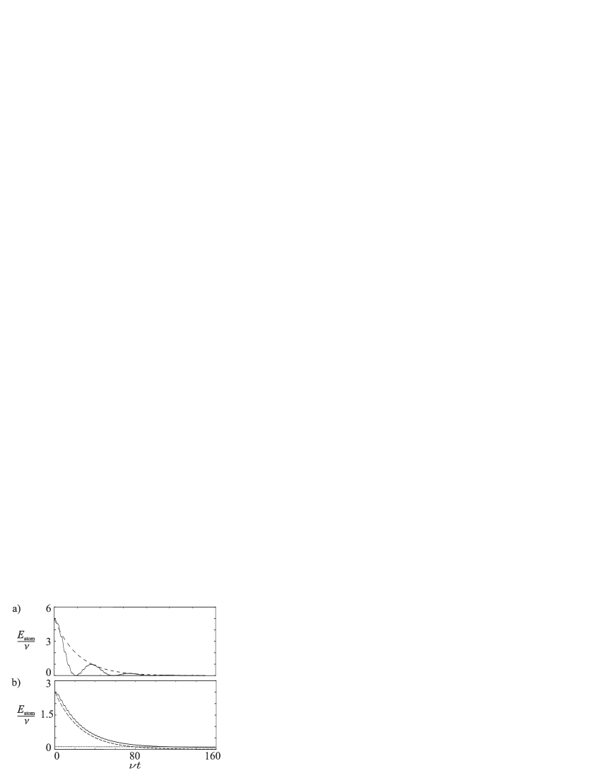
Figure 5: Energy of the atomic motion $E_{\rm atom}/\nu$ versus time $\nu t$. The parameters are chosen a) $\kappa=0.1$, $\nu=\nu_{c}=1$, $g_{\rm eff}=0.1$ and b) $\kappa=1$, $\nu=\nu_{c}=1$ and $g_{\rm eff}=0.1$. The dashed curves show an exponential decay with using the analytical expression for $\tau$. The dotted line in b) gives the analytical value for the final energy $E_{0}/\nu$.

In Fig. 5 we compare the analytical results for the cooling rates and the final temperatures with the exact numerical solution in two typical examples. One can see that the cooling times which we have estimated by using Eq. (13), fit the exact numerical calculations very well, and the final state temperature (which is almost zero in Fig. 5a coincides exactly with the analytical value calculated from Eq. (17).

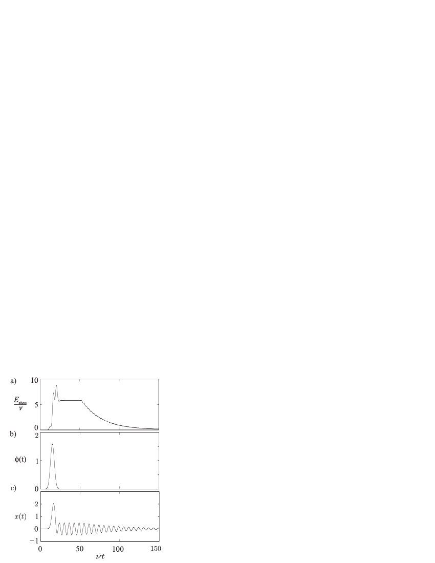
Figure 6: a) Energy of the atomic motion $E_{\rm atom}/\nu$ versus time $\nu t$. Initially the atom is in its motional ground state, then motional excitations are created by non adiabatic acceleration of the lattice. Afterwards cooling is switched on at $\nu t=51$ with parameters $\kappa=1$, $\nu=\nu_{c}=1$ and $g_{\rm eff}=0.1$. b) Expectation value $x(t)=\left\langle\hat{x}(t)\right\rangle$ of the atomic position in dimensionless units and c) the relative phase $\phi(t)$ between the two lasers.

Finally, Fig. 6 shows the excitation of the motional state of an atom, initially assumed to be in its motional ground state, by non adiabatic acceleration of the lattice. The chosen velocity profile is typical for a two qubit quantum gate where one atom is moved close to a second one for performing the gate operation. While here we assume that the motional state is excited during one such movement it might typically only be necessary to re-cool the atom after a few gate operations have been performed. After the motion has finished we turn on the cooling to bring the atom back into its motional ground state. The results are summarized in Fig. 6. The time evolution of the atomic energy

$$E_{A}=\nu\left\langle c^{\dagger}c\right\rangle-\frac{\nu\alpha}{2}\left(\left\langle c\right\rangle+\left\langle c^{\dagger}\right\rangle\right)+\frac{\nu^{2}}{4}\alpha^{2}-\frac{\rmi\nu\dot{\alpha}}{2}\left(\left\langle c^{\dagger}\right\rangle-\left\langle c\right\rangle\right)+\frac{\nu^{2}\dot{\alpha}}{4},$$ (20)

which includes the kinetic energy part due to the motion as well as the vibrational excitation inside the trap is shown in Fig. 6a. The motion of the optical lattice is caused by a time dependent relative phase $\phi(t)=kx_{0}(t)$ (c.f. Fig. 6b) with $x_{0}(t)$ the mean equilibrium position of the atom. During the acceleration, the mean atomic position $x(t)=\left\langle\hat{x}(t)\right\rangle$, shown in Fig.6c, follows its equilibrium position $x_{0}(t)$ quite well. After the acceleration has stopped and the cooling has been turned on the motion of the atom is cooled down to the temperature $T_{f}$ (Eq.17) within a few trap periods.

4 Imperfections

In this section we discuss sources of imperfections leading to qubit errors for a specific internal level structure of the neutral atoms storing the qubits. We consider the fine structure levels of an alkali atom as e.g. Na or Rb shown in Fig. 7 and the laser light ideally travelling along the quantization axis $z$. We assume the qubit state $\left|0\right\rangle$ ($\left|1\right\rangle$) to be encoded in the $m_{j}=-1/2$ ($m_{j}=+1/2$) state of the $S_{\frac{1}{2}}$ manifold. This qubit state is coupled to the excited state $m_{j}=-3/2$ ($m_{j}=+3/2$) of the $P_{\frac{3}{2}}$ manifold by a $\sigma^{-}$ ($\sigma^{+}$) polarized laser with detuning $\Delta_{1}$ ($\Delta_{2}$). We consider two kinds of imperfections (i) qubit flip errors due to misalignment of the laser leading to small errors in the polarization vector $\delta{\bf\epsilon}$ and (ii) stray magnetic fields $\delta{\bf B}$ parallel to the quantization axis or equivalently imbalances in the two Rabi frequencies leading to qubit phase errors, i.e. the accumulation of a relative phase between $\left|0\right\rangle$ and $\left|1\right\rangle$ during the cooling process.

The probability $P_{\rm flip}$ for a spin flip error ($\left|0\right\rangle\leftrightarrow\left|1\right\rangle$) to occur in a given time interval $\tau$ is found to be

$$P_{\rm flip}=\frac{\Omega^{4}}{18\Delta^{2}}\tau^{2}\delta\epsilon_{3}^{2},$$ (21)

where $\delta\epsilon_{3}$ is the component of the polarization vector in the direction of the quantization axis. Inserting typical values $\tau\sim 20/\nu$ (cooling time found for the parameters used in Fig. 4) and $\delta\epsilon_{3}\sim 10^{-4}$ we find $P_{\rm flip}\sim 10^{-3}$.

A magnetic field in $z$-direction $\delta B_{3}$ leads to a Zeeman shift $\delta E=gm_{j}\mu_{B}\delta B$, with $\mu_{B}$ denoting the Bohr magneton and $g$ the Landé factor of the different states. The resulting difference in the transition frequencies from $\left|0\right\rangle\leftrightarrow\left|e_{1}\right\rangle$ and $\left|1\right\rangle\leftrightarrow\left|e_{2}\right\rangle$ leads to two different Stark shifts $\Omega^{2}/\Delta_{1}$ and $\Omega^{2}/\Delta_{2}$. Note that imbalances in the Rabi frequencies or differences in the trapping potentials of the two qubit states also lead to differences in these Stark shifts and can thus be treated in an identical way. The relative phase accumulated in time $\tau$ is given by

$$\phi_{\rm rel}=\frac{\Omega^{2}}{2\Delta_{2}^{2}}\tau\mu_{B}\delta B_{3}.$$ (22)

For the typical values used above and $\delta B_{3}\sim 1G$ we obtain a relative phase $\phi_{\rm rel}\sim 5\times 10^{-3}$.

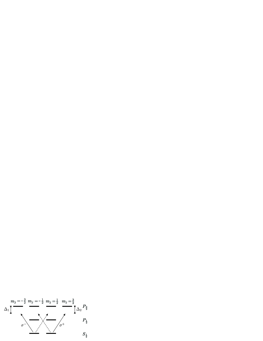
Figure 7: Fine structure and laser configuration as described in the text.

5 Conclusion

In this paper we have studied the nondestructive cooling of atomic qubits in an optical lattice by coupling to a dissipative optical cavity. In particular, we have proposed two specific experimental configurations, where the optical lattice was produced in the interior of an optical cavity, and the required dissipative mechanism was provided by photon loss through the mirrors of the cavity. In the first setup two counter-propagating laser beams were driving two modes of a ring cavity, resulting in an intra-cavity standing wave. We interpreted the resulting cooling in terms of a dissipative optical lattice which by an appropriate choice of atomic states became independent of the qubit state. In the second setup the ring cavity was replaced by a standing wave cavity and an optical potential was generated by two counter-propagating external laser beams intersecting the cavity at a small angle. In both cases the physics of cooling could be described as two coupled oscillators consisting of the phonon mode coupled parametrically to the optical cavity mode, which was damped by cavity loss providing the dissipative element for the cooling process.

Transport of $N$ atoms in the lattice gives rise to coherent oscillations of the center-of-mass mode of all the atoms. Our cooling scheme cools this particular collective mode with high efficiency due to the collective enhancement $g_{\rm eff}\rightarrow g_{\rm eff}\sqrt{N}$ of the coupling of the phonon to the photon modes. We find cooling times which are similar to those observed for other schemes [11] and are much smaller than the relevant decoherence times for the internal atomic states used in quantum information processing with neutral atoms. Therefore our scheme can be applied repeatedly to cool the motion of atoms which was excited during gate operations that involved moving the atoms. While the present work has emphasized application of this cooling scheme in a quantum information context, coupling the motion of atoms in optical lattices to photon modes of a cavity might also be interesting from the perspective of quantum degenerate gases in optical lattices.

Appendix A Transformation to a Classical Driving Field

We describe the transformation which allows the incident field to be represented by a classical driving field in the Hamiltonian (1), similar to the work by Mollow [29]. The state vector $\left|\psi(t)\right\rangle$ giving the system and the driving field satisfies the Schrödinger equation

$$\rmi\frac{\rm d}{{\rm d}t}\left|\psi(t)\right\rangle=H\left|\psi(t)\right\rangle,$$ (23)

where $H$ is given by Eq. (1). The initital state is assumed to be a product state of the system and a coherent field state

$$\left|\psi(0)\right\rangle=\left|\psi_{\rm sys}(0)\right\rangle\otimes D(\{\beta_{\omega,R},\beta_{\omega,L}\})\left|\rm vac\right\rangle,$$ (24)

where $\left|\rm vac\right\rangle$ is the vacuum state and

$$D(\{\beta_{\omega,R},\beta_{\omega,L}\})=\exp\left(\sum_{j=R,L}\int{\rm d}\omega\left(\beta_{\omega,j}b_{\omega,j}^{\dagger}-\beta_{\omega,j}^{*}b_{\omega,j}\right)\right)$$ (25)

is the coherent displacement operator (see e.g. [29]). In order to transform the coherent incident field to a classical driving field we apply the unitary transformation

$$\left|\psi(t)\right\rangle\rightarrow D^{\dagger}(\{\beta_{\omega,R}\rme^{-\rmi\omega t},\beta_{\omega,L}\rme^{-\rmi\omega t}\})\left|\psi(t)\right\rangle,$$ (26)

which results in an initial vacuum state for the driving field and in the transformation $b_{\omega,R(L)}\rightarrow b_{\omega,R(L)}+\beta_{\omega,R(L)}\rme^{-\rmi\omega t}$. Assuming symmetric driving $\beta_{\omega,R}=\beta_{\omega,L}\equiv\beta_{\omega}$ the Hamiltonian now has the form Eq. (1) with the additional term $\widetilde{H}_{\rm CF}$ defined in Eq. (3) and we have used

$$\beta_{\rm in}(t)=\frac{1}{\sqrt{2\pi}}\int{\rm d}\omega\rme^{\rmi(\omega_{L}-\omega)t}\beta_{\omega}.$$ (27)

Appendix B Damping Equations

The Heisenberg equations for the expectation values of the second order moments can be obtained from the master equation (4) with the system Hamiltonian Eq. (12), yielding

$$\frac{\rmd}{\rmd t}{\left\langle c^{\dagger}c\right\rangle}=g_{\rm eff}\left(\left\langle ca\right\rangle-\left\langle ca^{\dagger}\right\rangle-\left\langle c^{\dagger}a\right\rangle+\left\langle c^{\dagger}a^{\dagger}\right\rangle\right),$$ (28)

$$\frac{\rmd}{\rmd t}{\left\langle a^{\dagger}a\right\rangle}=g_{\rm eff}\left(\left\langle ca\right\rangle+\left\langle ca^{\dagger}\right\rangle+\left\langle c^{\dagger}a\right\rangle+\left\langle c^{\dagger}a^{\dagger}\right\rangle\right),$$

$$\frac{\rmd}{\rmd t}{\left\langle ca\right\rangle}=g_{\rm eff}\left(\left\langle c^{\dagger}c\right\rangle+\left\langle a^{\dagger}a\right\rangle+\left\langle c^{2}\right\rangle-\left\langle a^{2}\right\rangle\right)+(-\rmi\nu-\rmi\nu_{c}-\frac{\kappa}{2})\left\langle ca\right\rangle+g_{\rm eff},$$

$$\frac{\rmd}{\rmd t}{\left\langle ca^{\dagger}\right\rangle}=g_{\rm eff}\left(\left\langle c^{\dagger}c\right\rangle-\left\langle a^{\dagger}a\right\rangle+\left\langle c^{2}\right\rangle+\left\langle a^{\dagger^{2}}\right\rangle\right)+(-\rmi\nu+\rmi\nu_{c}-\frac{\kappa}{2})\left\langle ca^{\dagger}\right\rangle,$$

$$\frac{\rmd}{\rmd t}{\left\langle c^{\dagger}a\right\rangle}=g_{\rm eff}\left(\left\langle c^{\dagger}c\right\rangle-\left\langle a^{\dagger}a\right\rangle+\left\langle c^{\dagger^{2}}\right\rangle-\left\langle a^{2}\right\rangle\right)+(\rmi\nu-\rmi\nu_{c}-\frac{\kappa}{2})\left\langle c^{\dagger}a\right\rangle,$$

$$\frac{\rmd}{\rmd t}{\left\langle c^{\dagger}a^{\dagger}\right\rangle}=g_{\rm eff}\left(\left\langle c^{\dagger}c\right\rangle+\left\langle a^{\dagger}a\right\rangle+\left\langle c^{\dagger^{2}}\right\rangle-\left\langle a^{\dagger^{2}}\right\rangle\right)+(\rmi\nu+\rmi\nu_{c}-\frac{\kappa}{2})\left\langle c^{\dagger}a^{\dagger}\right\rangle+g_{\rm eff},$$

$$\frac{\rmd}{\rmd t}{\left\langle c^{2}\right\rangle}=2g_{\rm eff}\left(-\left\langle ca\right\rangle+\left\langle ca^{\dagger}\right\rangle\right)+2\rmi\nu\left\langle c^{2}\right\rangle,$$

$$\frac{\rmd}{\rmd t}{\left\langle a^{2}\right\rangle}=2g_{\rm eff}\left(\left\langle ca\right\rangle+\left\langle c^{\dagger}a\right\rangle\right)+\left(-2\rmi\nu_{c}-\kappa\right)\left\langle a^{2}\right\rangle,$$

$$\frac{\rmd}{\rmd t}{\left\langle c^{\dagger^{2}}\right\rangle}=2g_{\rm eff}\left(\left\langle c^{\dagger}a\right\rangle-\left\langle ca^{\dagger}\right\rangle\right)+2\rmi\nu\left\langle c^{\dagger^{2}}\right\rangle,$$

$$\frac{\rmd}{\rmd t}{\left\langle a^{\dagger^{2}}\right\rangle}=2g_{\rm eff}\left(\left\langle c^{\dagger}a^{\dagger}\right\rangle+\left\langle ca^{\dagger}\right\rangle\right)+\left(2\rmi\nu_{c}-\kappa\right)\left\langle a^{\dagger^{2}}\right\rangle.$$

In RWA the time evolution of the expectation values of the quadratic operators is given by a homogeneous set of linear differential equations, which can be written in the form

$$\frac{\rmd}{\rmd t}{\vec{y}(t)}=\mathcal{M}\vec{y}(t).$$ (29)

Here $\vec{y}(t)$ is given by

$$\vec{y}(t)=\left(\left\langle c^{\dagger}c\right\rangle,\left\langle a^{\dagger}a\right\rangle,\left\langle ca^{\dagger}\right\rangle,\left\langle c^{\dagger}a\right\rangle\right)^{\rm T},$$ (30)

and the time evolution matrix $\mathcal{M}$ has the form

$$\mathcal{M}=\left(\begin{array}[]{cccc}0&0&-g_{\rm eff}&-g_{\rm eff}\\ 0&-\kappa&g_{\rm eff}&g_{\rm eff}\\ g_{\rm eff}&-g_{\rm eff}&\rmi(\nu_{c}-\nu)-\frac{\kappa}{2}&0\\ g_{\rm eff}&-g_{\rm eff}&0&\rmi(\nu-\nu_{c})-\frac{\kappa}{2}\\ \end{array}\right).$$ (35)

References

References

- [1] J.I. Cirac, L.M. Duan, D. Jaksch and P. Zoller Proceedings of the International School of Physics “Enrico Fermi” Course CXLVIII, Experimental Quantum Computation and Information, IOS Press (2002).
- [2] D.Kielpinski, C.Monroe and D.J.Wineland , Nature 417, 709 (2002).
- [3] J.I.Cirac and P.Zoller, Nature 404, 579 (2000).
- [4] D. Kielpinski, B. E. King, C. J. Myatt, C. A. Sackett, Q. A. Turchette, W. M. Itano, C. Monroe, D. J. Wineland, and W. H.Zurek, Phys. Rev. A 61, 032310 (2000).
- [5] J. Eschner, G. Morigi, F. Schmidt-Kaler and R. Blatt J. Opt. Soc. Am. B 20, 1003 (2003).
- [6] H.J. Metcalf and P. van der Straten, J. Opt. Soc. Am. B 20, 909 (2003).
- [7] D. Jaksch, H.-J. Briegel, J.I. Cirac, C.W. Gardiner and P. Zoller Phys. Rev. Lett. 82, 1975 (1999)
- [8] O. Mandel, M. Greiner, A. Widera, T. Rom, T.W. Hänsch and I. Bloch, Phys. Rev. Lett 91, 010407 (2003).
- [9] O. Mandel, M. Greiner, A. Widera, T. Rom, T. W. Hänsch, and I. Bloch quant-ph/0308080 (2003).
- [10] G.K.Brennen, C.M.Caves, P.S.Jessen and I.H.Deutsch, Phys. Rev. Lett. 82, 1060 (1999).
- [11] A. J. Daley, P. O. Fedichev and P. Zoller, quant-ph/0308129 (2003).
- [12] T. Pellizzari, S. A. Gardiner, J. I. Cirac, and P. Zoller, Phys. Rev. Lett. 75, 3788 (1995).
- [13] A. S. Parkins, H. J. Kimble, Phys. Rev. A 61, 052104 (2000).
- [14] S. van Enk, J. I. Cirac, P. Zoller, H. J. Kimble, and H. Mabuchi, J. Mod. Opt. 44, 1727 (1997).
- [15] Philippe Grangier, Georges Reymond, Nicolas Schlosser, Fortschritte der Physik 48, 859 (2000).
- [16] A. Hemmerich, Phys. Rev. A 60, 943 (1999).
- [17] P.Domokos and H.Ritsch, JOSA B 20, 1098 (2003).
- [18] V.Vuletić and S.Chu, Phys. Rev. Lett 84, 3787 (2000).
- [19] P.W.H. Pinkse, T. Fischer, P. Maunz, and G. Rempe Nature 404, 365 (2000).
- [20] C. J. Hood, T. W. Lynn, A. C. Doherty, A. S. Parkins, and H. J. Kimble, Science 287, 1447 (2000).
- [21] D. Kruse, M. Ruder, J. Benhelm, C. von Cube, C. Zimmermann, Ph.W. Courteille, Th. Elsässer, B. Nagorny, and A. Hemmerich, Phys. Rev. A 67, 051802(R) (2003).
- [22] B. Nagorny, Th. Elsässer, H. Richter, A. Hemmerich, D. Kruse, C. Zimmermann, and Ph. Courteille, Phys.Rev A 67 031401(R) (2003).
- [23] Th. Elsässer, B. Nagorny, A. Hemmerich Phys.Rev A 67 051401 (2003).
- [24] D.F. Walls and G.J. Milburn, Quantum Optics, Springer Berlin Heidelberg (1994).
- [25] C.W. Gardiner and P. Zoller, Quantum Noise, Springer Berlin Heidelberg (2000).
- [26] P. Horak and H. Ritsch, Phys. Rev. A 64,033422 (2001).
- [27] M. Gangl and H. Ritsch, Phys. Rev. A 61,011402 (2000).
- [28] H.J. Metcalf and P. van der Straten, Laser Cooling and Trapping, Springer New York (1999).
- [29] B. R. Mollow, Phys. Rev. A 12, 1919 (1975).