Entanglement and Frustration in Ordered Systems

Abstract

This article reviews and extends recent results concerning entanglement and frustration in multipartite systems which have some symmetry with respect to the ordering of the particles. Starting point of the discussion are Bell inequalities: their relation to frustration in classical systems and their satisfaction for quantum states which have a symmetric extension. It is then discussed how more general global symmetries of multipartite systems constrain the entanglement between two neighboring particles. We prove that maximal entanglement (measured in terms of the entanglement of formation) is always attained for the ground state of a certain nearest neighbor interaction Hamiltonian having the considered symmetry with the achievable amount of entanglement being a function of the ground state energy. Systems of Gaussian states, i.e. quantum harmonic oscillators, are investigated in more detail and the results are compared to what is known about ordered qubit systems.

1 Introduction

Entanglement is the type of correlations which can be shared only with a finite number of parties—or to express it with the words of C.H. Bennett: ”Entanglement is monogamous“ (cf. [1]). This is maybe one of the main characteristics of entanglement and it clearly distinguishes entanglement from classical correlations. The present paper is devoted to investigate this ”monogamy property“ of entanglement in symmetric multipartite systems with the particular focus on the relation to frustration, the existence of local hidden variable models and to ground states of Hamiltonians having the considered symmetry. The article is based on a talk given at the QIT-EQIS workshop in Kyoto 2003 and it essentially reviews and extends results from [2] and [3, 4, 5].

In order to understand a characteristic feature of entanglement it is useful to study the counterpart in classical correlations first—this will clarify the difference between the quantum and the classical world. To this end Sec.2 will as a starting point discuss frustration in classical systems and their relation to Bell inequalities. In Sec.3 we will then utilize these observations in order to prove in a simple way that there exists a local hidden variable model for quantum states having symmetric extensions. Sec.4 considers more general symmetries and investigates the relation between the problem of maximizing the entanglement between nearest neighbors under a global symmetry constraint (e.g. translational symmetry) and the task of calculating ground state energies of certain nearest neighbor interaction Hamiltonians. Finally, Sec.5 will apply the ideas of the preceding section to Gaussian systems with symmetries characterized by symmetric graphs.

2 Bell inequalities and frustration in classical systems

Constraints on the possible range of correlations in the form of inequalities have been investigated for many years, even before physicists developed an interest in that subject due to the work of Bell [6] (see the monograph by Fréchet [7]). The relation between Bell inequalities and frustration in classical systems was then pointed out and studied in the early eighties in particular by Fine [3].

In spite of the simplicity of this connection there are, however, surprisingly many publications in the field of quantum information theory in which this knowledge has apparently disappeared. The following section will recall the relations between joint distributions, local hidden variable models, frustration and Bell inequalities.

2.1 Frustration in classical systems is due to loops

Let us consider a set of observables $X_{1},\ldots,X_{n}$ described within classical probability theory and let us denote the probability that observable $X_{i}$ leads to the outcome $x$ by $P_{X_{i}}(x)$. Obviously, there exists always a joint probability distribution $P_{X_{1},\ldots,X_{n}}=\prod_{i}P_{X_{i}}$ which returns all the single distributions as marginals. However, if we fix in addition the pair distributions $P_{X_{i},X_{j}}$ for a certain subset of pairs $(i,j)$ in a non-trivial way, a joint distribution with these marginals in general no longer exists. A necessary condition for the existence of $P_{X_{1},\ldots,X_{n}}$ is of course the compatibility of overlapping distributions in the sense that

$$\sum_{x_{2}}P_{X_{1},X_{2}}(x_{1},x_{2})=\sum_{x_{3}}P_{X_{1},X_{3}}(x_{1},x_{3})=P_{X_{1}}(x_{1}).$$ (1)

However, it is in general not sufficient, and the standard counter-example is a set of three observables with three pair distributions corresponding to total anti-correlations.

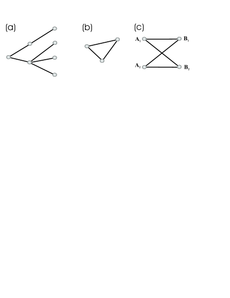
Figure 1: Frustration in classical systems is due to loops. Let the vertices and edges of a graph be assigned to observables and given pair distributions (correlations) respectivley. Then (a) for tree graphs there exists always a joint distribution returning all the given distributions as marginals, (b) loops may cause frustration and (c) a necessary and sufficient condition for the existence of a joint distribution in a two-colorable graph is given by Bell’s inequalities.

It is very useful to depict the problem graphically and to assign a vertex to every observable and an edge to each of the fixed pair distributions. In this picture, compatibility of the pair distributions is sufficient for the existence of a joint distribution $P_{X_{1},\ldots,X_{n}}$ if the graph does not contain any loops:

Proposition 1

Consider a graph, such that every vertex $k$ corresponds to one of $n$ observables $X_{k}$ and every edge $(k,l)$ corresponds to a given pair distribution $P_{X_{k},X_{l}}$. If all overlapping distributions are compatible in the sense of Eq.(1) and the graph does not contain any loop, then there exists a joint probability distribution $P_{X_{1},\ldots,X_{n}}$ which returns all the given distributions as marginals.

Proof: The proof can easily be formulated in terms of an induction. Assume there exists already a joint distribution $P_{X_{1},\ldots,X_{i}}$ which is compatible with all fixed pair distributions $P_{X_{k},X_{l}}$ where $k,l\leq i$ and has the same marginal $P_{X_{i}}$ as all given pair distributions $P_{X_{i},X_{j}}$ where $j>i$. Then we can construct a new distribution

$$P_{X_{1},\ldots,X_{i+1}}=P_{X_{1},\ldots,X_{i}}\;P_{X_{i},X_{i+1}}\;P^{-1}_{X_{i}}$$ (2)

which has all the required properties for a set of $i+1$ vertices. Since each step in the induction adds one edge and one vertex to the graph corresponding to the previous step, the construction only works for tree graphs, i.e., graphs without loops—otherwise one would at some point have to add an edge without adding a new vertex.

The final joint distribution is then given by

$$P_{X_{1},\ldots,X_{n}}=\left[\prod_{(k,l)}P_{X_{k},X_{l}}\right]\cdot\left[\prod_{j}P^{(1-e_{j})}_{X_{j}}\right],$$ (3)

where $e_{j}$ is the number of edges at the $j$’th vertex and the products have to be taken over all edges $(k,l)$ and vertices $j$ respectively.         

Prop. 1 shows that classically frustration is due to loops. This is in contrast to quantum mechanical systems, which can be frustrated even without loops.

2.2 Joint distributions and local hidden variable models

If the graph characterizing the fixed correlations between pairs of observables is two-colorable like in Fig.1(c) then a necessary and sufficient condition for the existence of a joint distribution is given by the complete set of Bell inequalities, i.e., by the existence of a local hidden variable model. In this sense the correlations of a quantum state which violates a Bell inequality lead to unresolvable frustration when described within classical probability theory.

Let us briefly recall the above mentioned result. We say that a set of measured correlations $\big{\{}P_{A_{i}B_{j}}\big{\}}$ between observables $A_{1},\ldots,A_{m_{A}}$ and $B_{1},\ldots,B_{m_{B}}$ admit a description within a local hidden variable model [3, 8, 9], if we can write

$$P_{A_{i}B_{j}}(a,b)=\int_{\Lambda}M(d\lambda)\chi_{A_{i}}(a,\lambda)\chi_{B_{j}}(b,\lambda).$$ (4)

Here $\lambda\in\Lambda$ is the hidden variable and the source of the correlation experiment is characterized by the probabilities with which the different $\lambda$ occur, i.e., by a probability measure $M$ on $\Lambda$. The response function $\chi_{A_{i}}(a,\lambda)$ gives the probability that measuring the system in state $\lambda$ with observable $A_{i}$ leads to the outcome $a$. The locality assumption in Eq.(4) is expressed in the fact that the response functions factorize, such that $\chi_{A_{i}}(a,\lambda)$ does not depend on $B_{j}$ and $\chi_{B_{j}}(b,\lambda)$ is independent of $A_{i}$.

The local hidden variable description of a set of correlations is equivalent to the existence of a joint probability distribution [3]:

Proposition 2

There exists a joint probability distribution for all given pair distributions $\big{\{}P_{A_{i}B_{j}}\big{\}}$ if and only if the correlations admit a description within a local hidden variable model.

Proof: Let $A=(A_{1},\ldots,A_{m_{A}})$, $a=(a_{1},\ldots,a_{m_{A}})$ be vectors of observables and their respective outcomes, and similarly for $B,\ b$. If $P_{A,B}$ is the joint distribution for all pair distributions $P_{A_{i},B_{j}}$, then

$$P_{A_{i},B_{j}}(\alpha,\beta)=\sum_{a,b}P_{A,B}(a,b)\;\delta_{\alpha,a_{i}}\;\delta_{\beta,b_{j}}$$ (5)

is an admissible (deterministic) local hidden variable model with $P_{A,B}$ playing the role of the measure $M$ and the two delta functions corresponding to the characteristic functions in Eq.(4).

Conversely, if $\big{(}\Lambda$, $M$, $\{\chi_{A_{i}}\}$, $\{\chi_{B_{j}}\}\big{)}$ are probability space, measure and response functions for a local hidden variable model, then

$$P_{A,B}(a,b)\equiv\int\!M(d\lambda)\prod_{i=1}^{m_{A}}\chi_{A_{i}}(a_{i},\lambda)\prod_{j=1}^{m_{B}}\chi_{B_{j}}(b_{j},\lambda)$$ (6)

is a joint distribution, which returns all pair distributions $P_{A_{i},B_{j}}$ as marginals.         

Note that Prop.2 naturally generalizes to $n$-partite systems, where correlations of the form $P_{A_{i}B_{j}\ldots N_{k}}$ instead of pair distributions are given.

3 Quantum states with symmetric extensions

As already mentioned frustration in quantum systems are possible even without loops in the configuration. The simplest example is a system of three qubits distributed to Alice, Bob and Charlie, where Alice wants to be maximally entangled with both her colleagues. Clearly, this is not possible and one way to see this is to realize that in such a scenario Alice could teleport an unknown qubit perfectly to both, Bob and Charlie, which contradicts the no-cloning theorem[10]. In fact, if Alice is maximally entangled with Bob she cannot share any correlations with Charlie, neither entanglement nor classical correlations and it has recently been proven that there is even a quantitative trade-off between the amount of entanglement Alice shares with Bob and the maximal amount of classical correlations shared with Charlie [11].

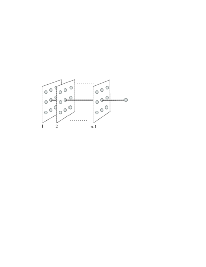
Figure 2: Consider a multipartite quantum systems composed out of a single particle (on the right) and $(n-1)$ “layers” of $m$ particles each. Assume complete permutation symmetry within each layer and let $\rho_{n}$ be the $n$-partite reduced state containing one particle of each layer plus the remaining single particle. Then $\rho_{n}$ admits a local hidden variable description for all correlations of an arbitrary number of observables on the $n$’th site and $m$ observables on each of the first $(n-1)$ sites.

We will in the following restrict to symmetric situations, where we have for instance Alice being surrounded by several Bobs and Charlies in a symmetric manner. Using the observations of the previous section, we can easily recover results of [4] and [5]:

Proposition 3

Let $\rho$ be a density matrix acting on a Hilbert space ${\cal H}_{A}\otimes{\cal H}_{B}^{\otimes m}$ such that all bipartite reduced states of the form $\rho_{AB_{j}}$ are equal. Then the state $\rho_{AB}\equiv\rho_{AB_{j}}$ admits a local hidden variable model with respect to all correlations between $m$ observables on site $B$ and an arbitrary number of observables measured on site $A$.

Proof: Let $\{F_{i}(a_{i})\}$, $\{G_{j}(b_{j})\}$ be the POVM operators corresponding to the measurement devices $A_{i}$ and $B_{j}$ with respective measurement outcomes $a_{i}$ and $b_{j}$. Then

$$P_{A_{i},B_{1},\ldots,B_{m}}(a_{i},b_{1},\ldots,b_{m})={\rm tr}\left[\rho F_{i}(a_{i})\otimes\bigotimes_{j=1}^{m}G_{j}(b_{j})\right]$$ (7)

is an admissible joint probability distribution compatible with all pair distributions $P_{A_{i},B_{j}}(a_{i},b_{j})={\rm tr}\left[\rho_{AB}F_{i}(a_{i})\otimes G_{j}(b_{j})\right]$. By applying Prop.1 and Prop.2 we have then that there exists a local hidden variable model for all correlations of an arbitrary number of observables acting on $A$ and $m$ measurement devices for $B$.         

Prop. 3 shows that if the number $m$ of equal neighbors in a quantum system is increased, then the bipartite correlations between the central particle and one of the neighbors become more and more classical. In fact, is was conjectured by Schumacher and proven by Werner (cf.[4, 12]) that if $m$ tends to infinity, then $\rho_{AB}$ cannot contain any entanglement—this is the only possibility of having a starlike extension with arbitrary many parties.

The following result generalizes Prop.3 to cases in which local hidden variable models for more than two parties can be constructed:

Proposition 4

Let $\rho$ acting on ${\cal H}^{\otimes N}$ be a density operator characterizing a state of $N=(n-1)m+1$ particles with permutation symmetry within each of $(n-1)$ disjoint sets of $m$ particles (see Fig.2). Take the $n$-partite reduced state $\rho_{n}$ which contains one particle of each set plus the remaining particle. Then $\rho_{n}$ admits a local hidden variable description for all correlations of an arbitrary number of observables on the $n$’th “single particle” site and $m$ observables on each of the remaining $(n-1)$ sites.

Proof: Let $\big{\{}F_{j}^{(i)}(a_{j}^{(i)})\big{\}}$ be the POVM corresponding to the $j$’th observable on site $i$ with respective outcome $a_{j}^{(i)}$. Then

$${\rm tr}\left[\rho\bigotimes_{k=1}^{m}\bigotimes_{i=1}^{n-1}F_{k}^{(i)}(a_{k}^{(i)})\otimes F_{j}^{(n)}(a_{j}^{(n)})\right]$$ (8)

is an admissible joint distribution for one observable ($j$) on the $n$’th site and $m$ observables on the remaining $(n-1)$ sites. Having the tensor factors properly ordered, this distribution is compatible with all correlations measured on $\rho_{n}$. This is seen by noting that taking the sum over $a_{k}^{(i)}$ in Eq.(8) corresponds to tracing out the $k$’th particle in the $i$’th set (“layer” in Fig.2). Due to the assumed permutation symmetry of $\rho$ it does, however, not matter which $(m-1)$ particles in each layer are traced out—we will always end up with the $n$-partite reduced state $\rho_{n}$.

By Prop.1 the probability distribution in Eq.(8) can be extended to a joint distribution including an arbitrary number of observables on the $n$’th site and by the multipartite generalization of Prop.2 there exists a local hidden variable model for all the considered correlations.         

4 Maximizing entanglement and minimizing energy

Prop. 3 and Prop. 4 show that an increasing symmetry of a quantum state (in the sense of an increasing number of equal neighbors) constrains the entanglement in such a way that violating Bell inequalities of a certain type is no longer possible. In the following we will consider multipartite quantum systems which have more general symmetries with respect to the ordering of the particles and investigate quantitatively how this global symmetry constraints the entanglement between two neighboring particles.

The considered symmetry group will always be a subgroup $G$ of the group ${\cal S}_{n}$ of all permutations of $n$ parties. The global density operator $\rho$ then commutes with all group elements and it is in particular invariant under the group averaging

$$\rho\mapsto{\cal T}(\rho):=\frac{1}{|G|}\sum_{g\in G}U_{g}\rho U_{g}^{\dagger}\;.$$ (9)

It is in many cases again advantageous to depict the problem graphically and to assume that the group $G$ is the symmetry group of a graph whose vertices correspond to particles, i.e., tensor factors of the total Hilbert space. For simplicity we will only consider edge transitive graphs here. This provides a natural notion of “neighboring” particles, namely those corresponding to adjacent vertices in the graph, and we will not have to specify which neighbors we are considering since they are all equal. Prominent examples of edge transitive graphs are stars, rings, cubic, hexagonal and trigonal lattices, permutational invariant clusters and the platonic solids.

Typically, states with these symmetries appear as ground states (or equilibrium states) of particles on a lattice with equal nearest neighbor interaction along the edges of the considered graph. We will show that the state which has the largest nearest neighbor entanglement under such a symmetry constraint is always the ground state of a certain nearest neighbor interaction Hamiltonian and that, moreover, the maximal achievable amount of entanglement is a function of the ground state energy.

This statement is rather obvious if we quantify the entanglement using a linear functional like the the overlap $f=\langle\Phi_{-}|\rho_{AB}|\Phi_{-}\rangle$ with the singlet state $\Phi_{-}$ of two qubits. In fact, in this case the maximum is always achieved for the ground state of the antiferromagnetic Heisenberg Hamiltonian, since we can write

$$|\Phi_{-}\rangle\langle\Phi_{-}|=\frac{1}{4}\Big{[}{\bf 1}-\sigma_{x}\otimes\sigma_{x}-\sigma_{y}\otimes\sigma_{y}-\sigma_{z}\otimes\sigma_{z}\Big{]}.$$ (10)

In this way we can for instance relate the ground state energy density of the infinite antiferromagnetic Heisenberg spin-$\frac{1}{2}$ chain to the maximal achievable singlet fraction of a state with infinite translation symmetry, which is then given by $f_{max}=\ln 2$.

However, an analogous statement is still true if we measure the entanglement in terms of a highly nonlinear functional, the entanglement of formation[14]. In contrast to the singlet fraction the entanglement of formation is a proper entanglement measure and it is closely related to the amount of pure state entanglement needed to prepare a state by means of local operations and classical communication. It is defined as

$$E_{F}(\rho_{AB})=\inf\left\{\sum_{i}p_{i}E(\Psi_{i})\Big{|}\sum_{i}p_{i}|\Psi_{i}\rangle\langle\Psi_{i}|=\rho\right\}\;,$$ (11)

where $E(\Psi)=S\big{(}{\rm tr}_{A}\big{[}|\Psi\rangle\langle\Psi|\big{]}\big{)}$ is the pure state entanglement of $\Psi$ given by the von Neumann entropy $S$ of the reduced state. Due to the fact that Eq.(11) is a so-called convex hull construction, we can prove the following:

Proposition 5

Consider the set ${\cal D}_{G}$ of multipartite quantum states with (permutation) symmetry group $G$ of an edge transitive graph. The maximal entanglement $E_{F}(\rho_{AB})$ between two neighboring particles of a state $\rho\in{\cal D}_{G}$ is attained for the ground state projector of a nearest neighbor interaction Hamiltonian with interactions along the edges of the considered graph. The maximal achievable entanglement is then a function of the ground state energy.

Proof: First note that by the concavity of the entropy we can take the infimum in Eq.(11) over all decompositions of $\rho_{AB}$ into mixed states $\{\sigma_{i}\}$ as well. Moreover, $E_{F}$ is by construction the convex hull of the functional $x\mapsto S\big{(}{\rm tr}_{A}[x]\big{)}$, which can equivalently be expressed as the supremum over all affine functions, which lie below it (cf.[15]). That is

$$E_{F}(\rho_{AB}) = \inf_{\{p_{i},\sigma_{i}\}}\left\{\sum_{i}p_{i}S\big{(}{\rm tr}_{A}[\sigma_{i}]\big{)}\Big{|}\sum_{i}p_{i}\sigma_{i}=\rho\right\}$$ (12)

$$= \sup_{h}\left\{{\rm tr}\left[\rho_{AB}h\right]\Big{|}\forall\sigma:{\rm tr}\left[\sigma h\right]\leq S\big{(}{\rm tr}_{A}[\sigma]\big{)}\right\}$$ (13)

$$= -\inf_{h}\left\{{\rm tr}\left[\rho_{AB}h\right]\Big{|}\forall\sigma:{\rm tr}\left[\sigma h\right]+S\big{(}{\rm tr}_{A}[\sigma]\big{)}\geq 0\right\}$$ (14)

$$= -\inf_{s}{\rm tr}\left[\rho_{AB}h(s)\right],$$ (15)

where $h(s)$ is a fictive parametrization of the set of “interactions” $h$ defined in Eq.(14).

By assumption $\rho_{AB}$ is a bipartite reduced state of a global state $\rho\in{\cal D}_{G}$ which is invariant under averaging over the group $G$. We can therefore write

$${\rm tr}\left[\rho_{AB}h(s)\right] = {\rm tr}\left[\rho\big{(}h(s)\otimes{\bf 1}\big{)}\right]={\rm tr}\left[{\cal T}\big{(}\rho\big{)}\big{(}h(s)\otimes{\bf 1}\big{)}\right]$$ (16)

$$= {\rm tr}\left[\rho{\cal T}\big{(}h(s)\otimes{\bf 1}\big{)}\right]=:{\rm tr}\left[\rho H(s)\right],$$ (17)

where $H(s)$ is a “Hamiltonian” with equal nearest neighbor interactions $h(s)$ along the edges of the considered graph. Due to the symmetry of $H(s)$ we can now drop the constraint $\rho\in{\cal D}_{G}$ in calculating the maximal achievable $E_{F}(\rho_{AB})$:

$$\sup_{\rho\in{\cal D}_{G}}E_{F}(\rho_{AB}) = -\inf_{s}\inf_{\tau}{\rm tr}\left[\tau H(s)\right]=-\inf_{s}e_{0}(s).$$ (18)

Here, $e_{0}$ is the ground state energy of the Hamiltonian $H(s)$ and the normalized projector onto the ground state space of the extremal Hamiltonian has then both, the required symmetry and the maximal entanglement properties.         

There are two drawbacks concerning the application of Prop.5. First of all, the parametrization of $h(s)$ is in general not known explicitly. In fact, there are only very few systems for which we are able to calculate $E_{F}(\rho_{AB})$. Besides highly symmetric one-parameter families of states [16, 17] this is at present only feasible for systems of two qubits [18] and symmetric two-mode Gaussian states [19].

The second problem is the calculation of the ground state energy $e_{0}(s)$ for large systems. Though some particular two-qubit interactions lead to exactly solvable models in one dimension, the set of these models is apparently not large enough in order to answer the question about the maximal possible $E_{F}(\rho_{AB})$ for an infinite qubit chain in a straight forward manner. Using results from Ref.[20] we can write the concurrence of two qubits (which is in turn a monotone function of $E_{F}$ [18]) as

$$c\big{(}\rho_{AB}\big{)}=\max\left\{0,-\inf_{\det{X}=1}{\rm tr}\left[\rho_{AB}(X\otimes X^{\dagger}{\bf F})\right]\right\},$$ (19)

where ${\bf F}$ is the flip operator. For a chain of qubits this leads to a somehow deformed XXZ + Z-field model which is, unfortunately, not exactly solvable.

However, for Hamiltonians which are quadratic in bosonic operators, i.e., interactions with Gaussian ground states, both problems—calculating $E_{F}$ (that is parameterizing $h(s)$) and calculating $e_{0}(s)$—are feasible.

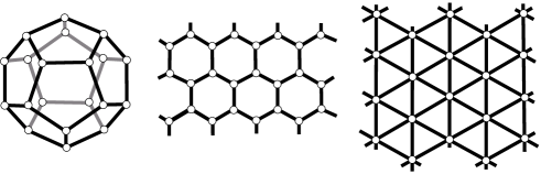
Figure 3: Examples of symmetric graphs are the five platonic solids (e.g. the dodecahedron) and the hexagonal and trigonal lattice. If every vertex corresponds to a single mode of a Gaussian state then the entanglement $E_{F}$ between nearest neighbors is maximized for the ground state of the nearest neighbor Hamiltonian given in Eq.(21). Although the entanglement is finite in each case, the respective ground states are infinitely squeezed.

5 Gaussian states on symmetric graphs

Let us consider a bosonic system of $n$ modes described by a set of canonical operators $(Q_{1},\ldots,Q_{n},P_{1},\ldots,P_{n})=:R$ obeying the canonical commutation relations $[Q_{k},P_{l}]=i\delta_{kl}{\bf 1}$. States with Gaussian Wigner distribution—so-called Gaussian states—are completely characterized by their first and second moments with respect to the canonical operators [21]. Physically they may describe modes of the electromagnetic field, atomic ensembles interacting with such fields, the motional state of a collection of ions in a trap or the low energy (bosonic) excitations of many other systems. All the information about correlations and entanglement properties of these states is contained in the covariance matrix

$$\Gamma_{kl}={\rm tr}\left[\rho\Big{\{}R_{k}-\langle R_{k}\rangle,R_{l}-\langle R_{l}\rangle\Big{\}}_{+}\right],$$ (20)

where $\langle R_{k}\rangle={\rm tr}\left[\rho R_{k}\right]$ and $\{\cdot,\cdot\}_{+}$ is the anti-commutator.

It was proven in Ref.[2] that for the case of Gaussian states on symmetric graphs, where every vertex corresponds to a single mode (one quantum harmonic oscillator), the Hamiltonian whose ground state maximizes $E_{F}(\rho_{AB})$ is of the form

$$H = \sum_{(k,l)}(Q_{k}+Q_{l})^{2}+(P_{k}-P_{l})^{2}$$ (21)

$$= \sum_{(k,l)}(a_{k}^{\dagger}a_{k}+\frac{1}{2})+\frac{1}{2}(a_{k}a_{l}+a_{k}^{\dagger}a_{l}^{\dagger})$$ (22)

$$=: \sum_{ij}h_{ij}R_{i}R_{j}\,$$ (23)

where the first two sums run over all edges $(k,l)$ of the graph and the Hamiltonian matrix $h\equiv h_{Q}\oplus h_{P}$ is block diagonal with the blocks $h_{Q}$ and $h_{P}$ being easily determined from the adjacency matrix of the graph. The ground state energy $e_{0}$ of the Hamiltonian and the covariance matrix of the respective ground state $\Gamma_{0}$ are then given by

$$e_{0}=||\sqrt{h_{Q}h_{P}}||_{1}\;,\qquad\Gamma_{0}=\sqrt{h_{P}h_{Q}^{-1}}\oplus\sqrt{h_{Q}h_{P}^{-1}}.$$ (24)

Although the entanglement is finite in all non-trivial cases all the ground states are infinitely squeezed, which is mathematically expressed in the fact that $\Gamma_{0}$ has zero eigenvalues.

Figure 4: The maximal achievable entanglement $E_{F}$ (ebits) between two particles in an $N$-partite permutational symmetric cluster. The lower curve corresponds to $N$-mode Gaussian states, and the upper curve shows the result for an $N$-qubit system. Both vanish asymptotically as $\sim\frac{1}{N^{2}}\log_{2}{N}$.

Figs. 5 and 4 show the (analytic) results for a translational invariant ring and a permutational invariant cluster of harmonic oscillators and compare them to what is known from the case of qubit systems. Surprisingly, the maximal value of $E_{F}$ is of the same order of magnitude for both systems and as it is expected for a ring of qubits, the ring of harmonic oscillators shows an odd-even oscillation with respect to the number of particles.

This together with other results from Ref.[2] indicates three different tendencies for the maximal $E_{F}$:

1. It decreases with the number of adjacent vertices.

2. It decreases with the total number of vertices.

3. It is suppressed in loops with an odd number of vertices, which give thus rise to additional frustration.

Figure 5: Maximal nearest neighbor entanglement (ebits) in a ring of $N$ harmonic oscillators (the dotted curves represent the envelopes). In the limit $N\rightarrow\infty$ this approaches $0.30$ ebits, which is comparable to the $0.29$ ebits Wootters found as a lower bound for the case of an infinite qubit chain.

References

- [1] B.M. Terhal, LANL quant-ph/0307120 (2003).
- [2] M.M. Wolf, F. Verstraete, J.I. Cirac, to appear in Phys. Rev. Lett.; LANL quant-ph/0307060 (2003).
- [3] A. Fine, J. Math. Phys. 23, 1306 (1982).
- [4] R.F. Werner, Lett. Math. Phys. 17, 359 (1989).
- [5] B. Terhal, A.C. Doherty, D. Schwab, Phys. Rev. Lett. 90, 157903 (2003).
- [6] J.S. Bell, Physics 1, 195 (1964).
- [7] M. Fréchet, Les Probabilités Associées a un Système D’Événtments Compatibles et Dépandants, Hermann, Paris (1940).
- [8] R.F. Werner, M.M. Wolf, Quant. Inf. Comp. 1(3), 1 (2001).
- [9] M.D. Mermin, Rev. Mod. Phys. 65, 803 (1993).
- [10] W.K. Wootters, W.H. Zurek., Nature 299, 802 (1982).
- [11] M. Koashi, A. Winter, LANL quant-ph/0310037 (2003).
- [12] A.C. Doherty, P.A. Parrilo, M. Spedalieri, LANL quant-ph/0308032 (2003).
- [13] T. Eggeling, R.F. Werner, M.M. Wolf, in preparation.
- [14] C.H. Bennett, D.P. DiVincenzo, J.A. Smolin, W.K. Wootters, Phys. Rev. A 54, 3824 (1996).
- [15] K.M.R. Audenaert, S.L. Braunstein, LANL quant-ph/0303045 (2003).
- [16] K.G.H. Vollbrecht, R.F. Werner, Phys. Rev. A 64, 062307 (2001).
- [17] B.M. Terhal, K.G.H. Vollbrecht Phys. Rev. Lett. 85, 2625 (2000).
- [18] W.K. Wootters, Phys. Rev. Lett. 80, 2245 (1998).
- [19] G. Giedke, M.M. Wolf, O. Krüger, R.F. Werner, J.I. Cirac Phys. Rev. Lett. 91, 107901 (2003).
- [20] F. Verstraete, J. Dehaene, B. De Moor Phys. Rev. A 65, 032308 (2002).
- [21] A.S. Holevo, Probabilistic and statistical aspects of quantum theory, North-Holland Publishing Company, (1982).
- [22] A. Einstein, B. Podolsky, N. Rosen, Phys. Rev. 47, 777 (1935).
- [23] M. Koashi, V. Buzek, N. Imoto, Phys. Rev. A 62, 050302(R) (2000).
- [24] W.K. Wootters, Contemp. Math. 305, 299 (2002); K. O’Connor, W.K. Wootters, Phys. Rev. A 63, 052302 (2001).