Vacuum-field atom trapping
in a wide aperture spherical resonator.

Abstract

We consider the situation where a two-level atom is placed in the vicinity of the center of a spherical cavity with a large numerical aperture. The vacuum field at the center of the cavity is actually equivalent to the one obtained in a microcavity, and both the dissipative and the reactive parts of the atom’s spontaneous emission are significantly modified. Using an explicit calculation of the spatial dependence of the radiative relaxation rate and of the associated level shift, we show that for a weakly excitating light field, the atom can be attracted to the center of the cavity by vacuum-induced light shifts.

I Introduction

Many theoretical and experimental work has been devoted during recent years to the so-called “cavity QED” regime, where strong coupling is achieved between a few atoms and a field mode contained inside a microwave or optical cavity. In particular, it has been demonstrated that the spontaneous emission rate of an atom inside the cavity is different from its value in free space note ; D ; K ; GRGH ; GD ; HHK ; HCTF ; JAHMMH ; DIJM ; ZLML ; HF ; MYM ; JMD1 . This effect can be discussed from several different approaches, and here it will be basically attributed to a change of the spectral density of the modes of the vacuum electromagnetic field, which is due to the cavity resonating structure JMD1 . This approach is particularly convenient when the cavity does not have one single high-finesse mode, but rather many nearly degenerate modes, as it is the case in confocal or spherical cavities. More precisely, we will show that a “wide aperture” concentric resonator using spherical mirrors with a large numerical aperture, can in principle change significantly the spontaneous emission rate of an atom sitting close to the cavity center, even with moderate finesse. Similar result were already demonstrated, using either a spherical cavity HCTF ; HF ; JMD1 or “hour-glass” modes in a confocal cavity MYM .

In such experiments, the atom has to sit within the active region volume, which is usually of very small size (of order $(10\lambda)^{3}$ to $(100\lambda)^{3}$). In refs HF ; MYM , a possible solution was implemented by using a narrow atomic beam, and by reducing the cavity finesse in order to have an extended area in which a spherical wave is “self-imaged” on itself. However, getting large effects will put more severe constraints both on the quality of the cavity and on the localisation of the atoms. A different way to implement the proposed scheme in a spherical cavity, that we would like to discuss in more detail here, is to use light-induced forces in order to attract the atom to the cavity center. A possible implementation could be to couple a light beam inside the cavity, and then to use the dipole force to hold the atoms in the right position, i.e., close to the cavity center. The effect of strong atom-cavity coupling on the dipole force has been studied theoretically MLG ; SC , and very interesting effects can be expected : since the atomic relaxation will be modified by the cavity, the balance between the trapping and heating effects of the dipole trap will be changed with respect to free space, which could result in an improvement of the trap itself.

A good understanding of these effects requires first to know the full space dependence of the cavity-induced damping and level shifts. In this letter, we will look at the situation where the atom lies close to the center of a spherical cavity with a large numerical aperture. We will show that large changes both in the atom damping rate and in its energy levels can be expected, even with a moderate cavity finesse, provided that the atom sits (relatively, but not extremely) close to the cavity center JMD1 . Moreover, we will show that for a weak excitating field, the atom can be trapped by vacuum-induced light shifts HBR ; ESBS , which create a force whose spatial dependence is related to the shape of the mode spectral density. In the following, we will assume that the cavity damping rate $\kappa$ is much larger than the free-space atom damping rate $\Gamma_{vac}$. In that case, the cavity still acts as a continuum with respect to the atomic relaxation. This will allow us to treat simply the atom-field coupling using frequency- dependant coupling coefficients. For simplicity, we will also assume a weak excitation of the atom. This assumption is however not crucial, and possible extensions will be discussed at the end of the paper.

II Light-induced forces in the cavity QED regime

Let us consider a neutral, slowly moving two-level atom in the dipole approximation. The Hamiltonian describing the atom-light coupling is :

$$H=H_{f}+H_{a}-{\bf D.E}({\bf r})$$ (1)

where $\bf D$ is the atom dipole moment and $\bf E$ is the electric field. The free field and atom hamiltonians are respectively $H_{f}=\sum_{k}\hbar\omega_{k}(n_{k}+1/2)$ and $H_{a}={\bf p}^{2}/(2m)+\hbar\omega_{o}S^{(z)}$. Here, $\bf r$ and $\bf p$ are the atom’s position and momentum, $m$ is its mass, and the dipole operator can be written ${\bf D}={\bf d}(e^{i\omega_{L}t}S^{(+)}+e^{-i\omega_{L}t}S^{(-)})$, where $S^{(+)}$ and $S^{(-)}$ are the usual two-level rising and lowering operators in the frame rotating at the angular frequency $\omega_{L}$ of an externally applied laser (we have $S^{(z)}=(S^{(+)}S^{(-)}-S^{(-)}S^{(+)})/2$). The electric field operator is expanded as usual on a basis of orthogonal modes, but we do not specify that these modes should be plane waves. One has therefore :

$${\bf E}({\bf r},t)=i\sum_{k}{\bf e}_{k}({\bf r})\;a_{k}(t)\;e^{-i\omega_{k}t}+h.c.$$ (2)

where $k$ is a mode label which include polarization, and ${\bf e}_{k}({\bf r})$ is the contribution of mode $k$ to the field at point ${\bf r}$ close to the cavity center. It will be convenient to refer optical frequencies to a reference $\omega_{L}$, which can be the frequency of an externally applied laser as said above, and to define :

$${\bf A}({\bf r},t)=i\sum_{k}{\bf e}_{k}({\bf r})\;a_{k}(t)\;e^{-i(\omega_{k}-\omega_{L})t}$$ (3)

so that :

$${\bf E}({\bf r},t)={\bf A}({\bf r},t)e^{-i\omega_{L}t}+{\bf A}^{\dagger}({\bf r},t)e^{i\omega_{L}t}.$$ (4)

Moving to a frame rotating at the frequency $\omega_{L}$ and using the rotating wave approximation, the interaction part of the Hamiltonian can be written :

$$H_{int}=-S^{(+)}{\bf d.A}-{\bf d.A^{\dagger}}S^{(-)}$$ (5)

From the expression of the hamiltonian one can simply get the force acting on the atomGA  :

$${\bf F}({\bf r},t)=\frac{d{\bf p}}{dt}=-{\bf\nabla}H={\bf\nabla}(S^{(+)}(t)\;{\bf d.A}({\bf r},t))+h.c.$$ (6)

In this expression, the only space-dependant part is ${\bf e}_{k}({\bf r})$, so the force can also be written :

$${\bf F}({\bf r},t)=i\;S^{(+)}(t)\;\sum_{k}{\bf\nabla}[\,{\bf d}.{\bf e}_{k}({\bf r})]\;a_{k}(t)\;e^{-i(\omega_{k}-\omega_{L})t}+h.c.$$ (7)

From the Hamiltonian, one gets the Heisenberg equations for the field operators $a_{k}$ CDG , which can be integrated formally, yielding (${\bf d}.{\bf e}_{k}$ is taken real) :

$$a_{k}(t)=a_{k}(t_{0})+\frac{{\bf d}.{\bf e}_{k}}{\hbar}\int_{0}^{t-t_{0}}d\tau S^{(-)}(t-\tau)e^{i(\omega_{k}-\omega_{L})(t-\tau)}$$ (8)

Using this result in the definition of the fields operators, one sees that the field splits in two parts ${\bf E}={\bf E_{o}}+{\bf E_{s}}$, where ${\bf E_{o}}$ and ${\bf E_{s}}$ are the well-known “vacuum field” and “source field” terms, which do not commute CDG . Similarly, the expression of the force splits in two parts :

$${\bf F}={\bf F_{o}}+{\bf F_{s}}$$ (9)

By choosing the normal ordering when separating the two non-commuting terms, the first part ${\bf F_{o}}$ gives the usual expression of the light-induced force GA . The second term ${\bf F_{s}}$ is zero in the absence of a cavity, because the gradient of the source field is zero at the dipole place. However, as we will show now, this is no longer true inside a cavity. Still assuming normal ordering, one gets :

$${\bf F_{s}} = \sum_{k}\frac{i\;{\bf\nabla}\left[{\bf d}.{\bf e}_{k}({\bf r})\right]\,{\bf d}.{\bf e}_{k}({\bf r})}{\hbar}\int_{0}^{t-t_{0}}d\tau S^{(+)}(t)S^{(-)}(t-\tau)\;e^{-i(\omega_{k}-\omega_{L})\tau}+h.c.$$ (10)

$$= {\bf\nabla}\left[\sum_{k}\frac{i\;({\bf d}.{\bf e}_{k}({\bf r}))^{2}}{2\hbar}\int_{0}^{t-t_{0}}d\tau S^{(+)}(t)S^{(-)}(t-\tau)\;e^{-i(\omega_{k}-\omega_{L})\tau}\right]+h.c.$$

In order to get the physical meaning of this integral, let us write the Heisenberg equation for $S^{(-)}$ and use the expression of $a_{k}$ in order to get :

$$\frac{dS^{(-)}}{dt}=i\delta_{L}S^{(-)}-2iS^{(z)}\frac{{\bf d}.{\bf A}_{o}}{\hbar}+2\sum_{k}\frac{({\bf d}.{\bf e}_{k})^{2}}{\hbar^{2}}\int_{0}^{t-t_{0}}d\tau S^{(z)}(t)S^{(-)}(t-\tau)e^{-i(\omega_{k}-\omega_{L})\tau},$$ (11)

where $\delta_{L}=\omega_{L}-\omega_{o}$. The integral appearing here has the same structure as the one appearing in eq. 10 under the gradient, and corresponds to the well known relaxation and light shift terms in the evolution of the dipole components. It can be calculated as usual using a Markov approximation CDG , which is possible here because as said above we assumed that the cavity features are wide compared to the free-space relaxation rate of the atom. In the weak excitation limit, which is assumed here, one can approximate the evolution of the correlation functions by their free evolution during the short memory time of the reservoir. Note that an extension should be made to the strong excitation regime by considering relaxation in a dressed state basis DC . Making the approximation $S^{(-)}(t-\tau)=S^{(-)}(t)\,e^{-i(\omega_{L}-\omega_{0})\tau}$ during the correlation time CDG , one can define the quantities :

$$\sum_{k}\frac{({\bf d.e}_{k}({\bf r}))^{2}}{\hbar^{2}}\int_{0}^{t-t_{0}}d\tau\;\;e^{-i(\omega_{k}-\omega_{o})\tau} = \sum_{k}\frac{({\bf d.e}_{k}({\bf r}))^{2}}{\hbar^{2}}\left(\pi\delta(\omega_{k}-\omega_{o})+i{\cal P}\left(\frac{1}{\omega_{k}-\omega_{o}}\right)\right)$$ (12)

$$= \Gamma({\bf r})/2+i\Delta({\bf r})$$

where one has therefore :

$$\Gamma({\bf r}) = \frac{2\pi}{\hbar^{2}}\sum_{k}({\bf d.e}_{k}({\bf r}))^{2}\delta(\omega_{k}-\omega_{o})$$ (13)

$$\Delta({\bf r}) = \sum_{k}\frac{({\bf d.e}_{k}({\bf r}))^{2}}{\hbar^{2}}{\cal P}\left(\frac{1}{\omega_{k}-\omega_{o}}\right)$$ (14)

Using these definitions and $S^{(z)}S^{(-)}=-S^{(-)}/2$, eq. 11 becomes as expected

$$\frac{dS^{(-)}}{dt}=(i\delta_{L}-i\Delta({\bf r})-\frac{\Gamma({\bf r})}{2})\;S^{(-)}-2iS^{(z)}\frac{{\bf d}.{\bf A}_{o}}{\hbar}$$ (15)

so that the atomic frequency $\omega_{0}$ becomes $\omega_{0}+\Delta({\bf r})$. We note that the free-space value of $\Delta({\bf r})$ is a diverging quantity, which is usually assumed to be absorbed in the definition of the atomic levels; therefore, one considers here only the (finite) change of $\Delta({\bf r})$ with respect to this free-space value, that will be denoted $\Delta^{\prime}({\bf r})$ :

$$\Delta^{\prime}({\bf r})=\Delta_{cav}({\bf r})-\Delta_{vac}({\bf r})$$ (16)

In the expression of the extra term in the force, one can use either $\Delta^{\prime}({\bf r})$ or $\Delta_{cav}({\bf r})$, since the gradient of $\Delta_{vac}({\bf r})$ is zero anyway, and one obtains finally :

$${\bf F_{s}} = \hbar/2\;\left(S^{(+)}S^{(-)}\;{\bf\nabla}(-\Delta^{\prime}({\bf r})+i\Gamma({\bf r})/2)+{\bf\nabla}(-\Delta^{\prime}({\bf r})-i\Gamma({\bf r})/2)\;S^{(+)}S^{(-)}\right)$$ (17)

$$= -\,{\bf\nabla}(\hbar\,\Delta^{\prime}({\bf r}))\;\;\Pi_{e}$$

where $\Pi_{e}=S^{(+)}S^{(-)}=S^{(z)}+1/2$ is the excited state population. Therefore the gradient of the cavity-induced light shift creates a force, which can attract the atom towards the cavity center for an appropriate choice of the atom-cavity detuning. Physically, it makes sense that ${\bf F_{s}}$ is also proportionnal to the excited level population. In order to characterize more precisely the behaviour of this force, one needs now the explicit space dependence of $\Delta^{\prime}({\bf r})$. The same calculation will also give the space-dependent damping $\Gamma({\bf r})/2$, which will be useful for calculating the steady state and evolution of the atomic operators.

III Cavity-induced relaxation rates and light shifts

For definiteness, we will consider the case of a spherical cavity of radius R and of reflectivity and transmittivity coefficients $\rho$ and $\tau$, with $\rho^{2}+\tau^{2}=1$, and $\tau^{2}=T$. We will assume that $kR\gg 1$ (typically $kR=10^{5}$), and a moderate cavity finesse (in the range 10-100). A crucial parameter is the solid angle subtended by the cavity, that will be denoted $\Delta\Omega_{cav}$. For instance, a cavity half-aperture angle of $45$ degrees gives ${\Delta\Omega_{cav}\over 4\pi}=0.3$, and therefore ${\Delta\Omega_{vac}\over 4\pi}=0.7$ as the fraction of space still occupied by vacuum modes. All parameters quoted above seem accessible from an experimental point of view, and we will show now that they allow one to get quite significant cavity-induced effects.

In order to calculate the explicit space and frequency dependence of the relaxation rate and level shift, we have followed two parallel approaches, which are described in detail in another publication JMD1 . The first one is to solve explicitly the field equations in a spherical geometry, taking into account the considerable simplifications which appear since we are interested in the field at distances smaller than $\sim 100\lambda\!\!\!\!{\makebox[1.0pt]{}^{-}}$ off the origin. In geometric optics this involves light-rays with an impact parameter smaller than $100\lambda\!\!\!\!{\makebox[1.0pt]{}^{-}}$, and therefore, in the multipole expansion of the field, it will be sufficient to consider harmonics up to order $l\leq 100$. Actually, up to $300$ harmonics have be used in order to check consistency. Another very important point is that the continuity equations of the fields on the mirrors must be expressed at a distance $R\simeq$ 1 cm. With $\lambda=780$ nm, this corresponds to $kR\simeq 80000$, which is quite large, and allows one to use asymptotic forms of the solutions on the mirrors. Under these assumptions, it can be shown that the expression of $\Delta^{\prime}({\bf r})$ and $\Gamma({\bf r})/2$ can be given an explicit operatorial form in the space of mode functions, and then evaluated numerically in a spherical harmonics basis JMD1 .

Besides this “exact” calculation, we have also looked for an approximate solution, inspired by ray-optics considerations, and eventually checked by comparison with the complete numerical calculation. Using this cross-checking method, we obtain finally that the effect of the cavity can be described to a very good approximation by the following formulas:

$${\Gamma({\bf r})\over\Gamma_{vac}}=\int_{4\pi}{d\hat{\Omega}\over 4\pi}\;\;{3\over 2}(1-({{\bf d}.\hat{\Omega}\over d})^{2})\big{(}{T\over\mid\!{1-\rho e^{2i\phi}}\!\mid^{2}}\cos^{2}\bigl{(}k\hat{\Omega}.{\bf r})\;+\;{T\over\mid\!{1+\rho e^{2i\phi}}\!\mid^{2}}\sin^{2}\bigl{(}k\hat{\Omega}.{\bf r})\big{)}$$ (18)

$${\Delta^{\prime}({\bf r})\over\Gamma_{vac}}=\int_{4\pi}{d\hat{\Omega}\over 4\pi}\;\;{3\over 2}(1-({{\bf d}.\hat{\Omega}\over d})^{2})\big{(}{\rho\;\sin(2\phi)\over\mid\!{1-\rho e^{2i\phi}}\!\mid^{2}}\cos^{2}\bigl{(}k\hat{\Omega}.{\bf r})\;-\;{\rho\;\sin(2\phi)\over\mid\!{1+\rho e^{2i\phi}}\!\mid^{2}}\sin^{2}\bigl{(}k\hat{\Omega}.{\bf r})\big{)}$$ (19)

where the notation $\hat{\Omega}$ describes a direction in space, while $\phi$ is a cavity detuning parameter that will be detailed below. These expressions have a straighforward interpretation, because they appear basically as integrals over the direction of light rays : in the integral over the directions, $\rho$ is the mirror reflectivity for rays subtended by the cavity, and is zero for rays outside the cavity solid angle. The different factors appearing in the integrals can be interpreted in the following way :

• The first factor under the integral corresponds to polarisation effects, taking into account the transverse character of the field.

• The second (resonance) factor is of the usual Fabry-Perot form, where $\phi$ is the cavity phase shift which includes first a term $\phi_{0}=\omega_{0}R/c$. The complete calculation shows that, in order to obtain a correct result outside the cavity center, $\phi$ should include also a contribution from spherical aberrations, that is : $\phi=\phi_{0}+\frac{k(r^{2}-(\hat{\Omega}.{\bf r})^{2})}{2R}$. This second term corresponds to the extra phase shift experienced by rays going through point ${\bf r}$ while propagating along the $\hat{\Omega}$ direction. The resonance factor has different expressions for the damping and the lamb shift terms, which correspond respectively to the active and reactive parts of the coupling. This is clearly apparent from the integrals of eq. 13 and 14, which involve either a delta function or a principal part. In the first case, the integration is trivial, and yields the resonance term of eq. 18, while in the second case the result is obtained by contour integration JMD1 , and gives the (dispersive) second term of eq. 19.

• The third term under the integrals is the stationnary wave pattern corresponding either to odd modes (with an anti-node in the center and a $\cos^{2}\bigl{(}k\hat{\Omega}.{\bf r})$ space dependence) or to even modes (with a node in the center and a $\sin^{2}\bigl{(}k\hat{\Omega}.{\bf r})$ space dependence).

• Finally, the integration over the mirrors is conveniently performed in spherical coordinates, by taking the $z$ axis along the cavity axis, and varying the azimuthal angle $\theta$ from $0$ to $\theta_{mirror}=\theta_{m}$. Improved accuracy (better than $1\%$) is obtained if one takes into account the fact that the rays which would be reflected near the edge of the mirror are actually lost due to diffraction and fail to do as many round-trips as the other ones. We have shown JMD1 that this effect can be taken into account very simply by decreasing $\theta_{m}$ to $\theta_{eff}=\theta_{m}-\delta\theta$, with $\delta\theta=1/\sqrt{kRT}$ for symmetrical mirrors.

The first results which can be obtained from the previous formulas are obviously the shift and damping at the cavity center, as a function of the atom-cavity detuning. For a dipole orientation parallel to the cavity axis, we obtain straightforwardly :

$${\Gamma_{par}({\bf 0})\over\Gamma_{vac}}={\Delta\Omega_{vac}\over 4\pi}(1+{\sin^{2}\theta_{m}\over 2})+{\Delta\Omega_{cav}\over 4\pi}(1-{\cos\theta_{m}(1+\cos\theta_{m})\over 2}){T\over\mid\!{1-\rho e^{2i\phi_{0}}}\!\mid^{2}}$$ (20)

$${\Delta^{\prime}_{par}({\bf 0})\over\Gamma_{vac}}={\Delta\Omega_{cav}\over 4\pi}(1-{\cos\theta_{m}(1+\cos\theta_{m})\over 2}){\rho\;\sin(2\phi_{0})\over\mid\!{1-\rho e^{2i\phi_{0}}}\!\mid^{2}}$$ (21)

while for a dipole orientation perpendicular to the cavity axis, we have :

$${\Gamma_{perp}({\bf 0})\over\Gamma_{vac}}={\Delta\Omega_{vac}\over 4\pi}(1-{\sin^{2}\theta_{m}\over 4})+{\Delta\Omega_{cav}\over 4\pi}(1+{\cos\theta_{m}(1+\cos\theta_{m})\over 4}){T\over\mid\!{1-\rho e^{2i\phi_{0}}}\!\mid^{2}}$$ (22)

$${\Delta^{\prime}_{perp}({\bf 0})\over\Gamma_{vac}}={\Delta\Omega_{cav}\over 4\pi}(1+{\cos\theta_{m}(1+\cos\theta_{m})\over 4}){\rho\;\sin(2\phi_{0})\over\mid\!{1-\rho e^{2i\phi_{0}}}\!\mid^{2}}$$ (23)

We note that these expressions yield for a randomly oriented dipole :

$${\Gamma_{av}({\bf 0})\over\Gamma_{vac}}={\Delta\Omega_{vac}\over 4\pi}+{\Delta\Omega_{cav}\over 4\pi}{T\over\mid\!{1-\rho e^{2i\phi_{0}}}\!\mid^{2}},\;\;\;{\Delta^{\prime}_{av}({\bf 0})\over\Gamma_{vac}}={\Delta\Omega_{cav}\over 4\pi}{\rho\;\sin(2\phi_{0})\over\mid\!{1-\rho e^{2i\phi_{0}}}\!\mid^{2}}$$ (24)

which have a straightforward interpretation in terms of resonant enhancement of the rays subtended by the cavity. We note that these results are the same as those given in ref. HCTF , up to factor two resulting from the fact that this reference was considering spatially averaged values rather than the peak value at the cavity center (see below for the space dependence). These functions are plotted on fig. 1 for ${\Omega_{cav}\over 4\pi}=0.3$ and $\rho=0.98$. It can be seen that very significant effects occur for these quite reasonable parameters, yielding more than 30-fold increase in the damping rate at the cavity center.

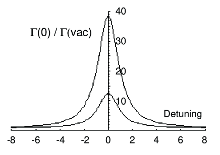
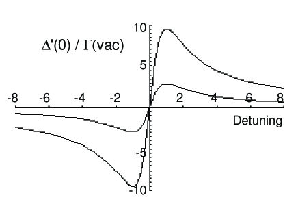
Figure 1: Normalized damping $\Gamma(0)/\Gamma_{vac}$ (left) and level shift $\Delta^{\prime}(0)/\Gamma_{vac}$ (right) at the cavity center, as a function of the atom-cavity detuning $(\omega_{0}-\omega_{cav})$ normalized to the cavity linewidth. The amplitude reflection coefficient of the mirrors is taken to be $\rho=0.98$, and the numerical aperture of the cavity is 0.7. The upper curves correspond to a dipole oriented perpendicular to the cavity axis, and the lower curves to a dipole oriented along the cavity axis.

We can then look at the results as a function of space for a given frequency, which are essential for the present paper. Two atom-cavity detunings are specially worth looking at : the resonant frequency at the cavity center, which yields maximum change in the damping rate but no cavity shift, and frequencies detuned by plus or minus half a cavity linewidth, which yield maximum cavity shifts. As an example, the results for the damping rates are plotted on fig. 2. The general values of the damping and level shifts for arbitrary values of the reflectivities $\rho_{1}$, $\rho_{2}$ of the two mirrors are given in JMD1 , Appendix C.

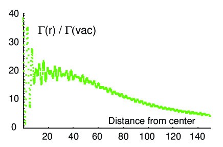
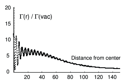
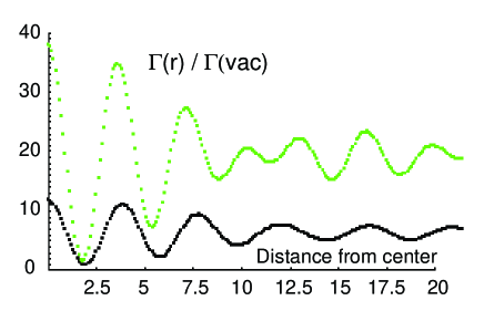
Figure 2: Spatial variation of the atomic damping $\Gamma(r)/\Gamma_{vac}$ on the cavity axis, obtained from the analytical formula given in the text. The atom-cavity detuning is taken equal to zero at the cavity center (see Fig. 1), and the horizontal axis unit is $1/k$. The amplitude reflection coefficient of the mirrors is $\rho=0.98$, and the numerical aperture of the cavity is 0.7. The upper left curve corresponds to a dipole oriented perpendicular to the cavity axis, the upper right curve to a dipole oriented along the cavity axis, and the lower curve is a zoom close to the cavity center.

IV Discussion

From the results of the previous section one can deduce some features of the “vacuum-induced” force given by eq. 17. For simplicity, we consider an atom at point $\bf{r}$ with zero velocity. The simplest configuration in which this force should be dominant is a weak stationnary wave resonant on the atom, but detuned from the cavity. In that case, both the usual scattering and dipole force are zero, while the cavity-induced light shift is maximum for a detuning of about half a cavity width. It can be seen easily that the force is attractive when the cavity is detuned to the blue side of the atomic resonance $(\omega_{0}<\omega_{cav})$ . This can be understood physically by realizing that the cavity “repels” the excited state level, and that this level has to go down in order to get an attractive potential. The corresponding potential wells are a few $\hbar\Gamma$ (see eq. 17), which is quite significant if cold atoms are used.

Besides the effect described here in the weak excitation regime, another possibility is to couple a laser beam inside the cavity, with a red atom-laser detuning, in order to create a dipole trap attracting the atom towards the cavity center. A very interesting effect can then be expected : since the atomic relaxation will be modified by the cavity, the balance between the trapping and heating effects of the dipole trap will be changed with respect to free space, enabling new regimes where the dipole force can be both attractive and damped. In that case, the calculation above should be extended to moving atoms (non-zero velocity) in order to calculate friction forces, as well as to calculate the diffusion coefficient. For very cold atoms, the quantum aspect of motion should also be included; this could be done in principle since we have obtained the explicit space dependence of the trapping potential.

V Conclusion

As a conclusion, we have shown that macroscopic cavities with large numerical apertures are interesting candidates for cavity QED experiments in the optical domain. The possibility to use light-induced force to hold the atom close to the cavity center is quite attractive, and it offers the possibility to study a well defined quantum system, including its external degrees of freedom. The expressions that we have obtained are general, and by using the results of ref. JMD1 they can be applied to any kind of low-finesse cavity, including the case of a “half-cavity” with only one mirror imaging the dipole onto itself inn1 ; inn2 ; inn3 .

References

- (1) Bibliographic note : this paper was written in 1995, and it is presented here in its original form with minor editing. The results were initially presented by Jean-Marc Daul at the conference “Quantum Optics in Wavelength Scale Structures”, Cargèse, Corsica, August 26-September 2, 1995. The same results were also presented by Philippe Grangier at the Annual Meeting of the TMR Network “Microlasers and Cavity QED”, Les Houches, France, April 21-25, 1997.
- (2) K.H. Drexhage in Progress in Optics XII, ed E. Wolf (North-Holland, Amsterdam, 1974).
- (3) D. Kleppner, Phys. Rev. Lett. 47, 233 (1981).
- (4) P. Goy, J.M. Raymond, M. Gross, and S. Haroche, Phys. Rev. Lett. 50, 1903 (1983).
- (5) G. Gabrielse and H. Dehmelt, Phys. Rev. Lett 55, 67 (1985).
- (6) R.G. Hulet, E.S. Hilfer, and D. Kleppner, Phys. Rev. Lett. 55 2137 (1985).
- (7) D.J. Heinzen, J.J. Childs, J.E. Thomas, and M.S. Feld, Phys. Rev. Lett. 58, 1320 (1987).
- (8) W. Jhe, A. Anderson, E.A. Hinds, D. Meschede, L. Moi and S. Haroche, Phys. Rev. Lett. 58, 666 (1987).
- (9) F. De Martini, G. Innocenti, G.R. Jacobovitz and P. Mataloni, Phys. Rev. Lett. 59 2955 (1987).
- (10) Y. Zhu, A. Lezama, T.W. Mossberg, and M. Lewenstein, Phys. Rev. Lett. 61, 1946 (1988).
- (11) D.J. Heinzen and M.S. Feld, Phys. Rev. Lett. 59, 2623 (1987).
- (12) S.E. Morin, C.C. Yu, and T.W. Mossberg, Phys. Rev. Lett. 73, 1489 (1994).
- (13) Jean-Marc Daul and Philippe Grangier, Cavity Quantum Electrodynamics in a wide aperture spherical resonator, Part I : Cavity-induced damping and level shifts, previous article (see also eprint quant-ph/0311047).
- (14) T.W. Mossberg, M. Lewenstein, and D.J. Gauthier, Phys. Rev. Lett. 67, 1723 (1991).
- (15) S. Haroche, M. Brune, J.M. Raimond, Europhys. Lett. 14, 19 (1991)
- (16) B.-G. Englert, J. Schwinger, A.O. Barut, and M.O. Scully, Europhys. Lett. 14, 25 (1991)
- (17) C. Cohen-Tannoudji, J. Dupont-Roc, G. Grynberg, “Atom-Photon Interactions. Basic Processes and Applications”, complement A.V, (Wiley, New York, 1992).
- (18) J. Dalibard, J. Dupont-Roc, and C. Cohen-Tannoudji, J. Physique, 43, 1617 (1982); 45, 637 (1984).63
- (19) J.P. Gordon and A. Ashkin, Phys. Rev. A 21, 1606 (1980).
- (20) J. Dalibard and C. Cohen-Tannoudji, J. Opt. Soc. Am. B 2, 1707 (1985).
- (21) C. Schön and J. I. Cirac, Phys. Rev. A 67, 043813 (2003)
- (22) J. Eschner, Ch. Raab, F. Schmidt-Kaler, and R. Blatt, Nature 413, 495-498 (2001).
- (23) M. A. Wilson, P. Bushev, J. Eschner, F. Schmidt-Kaler, C. Becher, R. Blatt, and U. Dorner, Phys. Rev. Lett. 91, 213602 (2003).
- (24) P. Bushev, A. Wilson, J. Eschner, C. Raab, F. Schmidt-Kaler, C. Becher, and R. Blatt, Phys. Rev. Lett. 92, 223602 (2004).