Robust High-Fidelity Teleportation of an Atomic State through the Detection of Cavity Decay

Abstract

We propose a scheme for quantum teleportation of an atomic state based on the detection of cavity decay. The internal state of an atom trapped in a cavity can be disembodiedly transferred to another atom trapped in a distant cavity by measuring interference of polarized photons through single-photon detectors. In comparison with the original proposal by S. Bose, P.L. Knight, M.B. Plenio, and V. Vedral [Phys. Rev. Lett. 83, 5158 (1999)], our protocol of teleportation has a high fidelity of almost unity, and inherent robustness, such as the insensitivity of fidelity to randomness in the atom’s position, and to detection inefficiency. All these favorable features make the scheme feasible with the current experimental technology.

PACS numbers: 03.67.-a, 42.50.Gy, 32.80.Qk

I introduction

Since the pioneering contribution of Bennett et al.[1], teleportation, which has recently attracted considerable attention as the means of disembodied transfer of an unknown quantum state, comes to be recognized as one of the basic methods of quantum communication and, more generally, lies at the heart of the whole field of quantum information. Experimental realizations of quantum teleportation have so far been focused on the discrete-variables case, which involves photonic polarization states[2, 3] and vacuum–one-photon states[4], as well as the continuous-variables one[5]. However, since atoms are favorable for the storage and processing of quantum information, teleportation of atomic states will be the next important benchmark on the way to obtaining a complete set of quantum information processing tools. Recently, a number of proposals[6, 7] based on cavity quantum electrodynamics (QED) have been presented for the teleportation of internal states of atoms. However, in the earlier ones[6], atoms, which are not suited for long distance transportation, have been used as flying qubits. From a practical point of view, photons are the best candidate for flying qubits as the fast and robust natural carriers of quantum information over long distance. In Ref.[7], Bose et al. designed a scheme for quantum teleportation with a successful combination of the two advantages: atoms act as stationary qubits, while photons play the role of flying qubits.

In this paper, we propose a scheme, which is similar to but more robust and efficient than that of Bose et al.[7], to teleport the internal state of an atom trapped in a cavity onto a second atom trapped in another distant cavity by detecting the photon decays from the cavities through single-photon detectors. Instead of fighting against the decay of the cavity field, which is seemed as a decoherence process resulting from the unavoidable interaction of the cavity system with its surroundings, we have designed an elegant scheme to use it as a constructive factor in the teleportation of an atomic state. This kind of idea was widely discussed and exploited very recently. Many schemes with this feature have been known for entangling two or more atoms[8, 9] as well as for entangling macroscopic atomic ensembles[10]. Related protocols for quantum gate operations and even universal quantum computation have also been proposed[11]. Most of these schemes are based on the detection of cavity decay and thus will succeed probabilistically only for particular measurement results.

Although quantum information is similarly carried by photonic states, our scheme is quite different from the previous quantum communication protocols[12]. In the proposals in Ref.[12], quantum information is directly transferred from an atom to another atom (both the atoms are trapped in cavities) through a photon, thus the high requirement for the experimental technology of feeding a photon into a cavity from the outside must be fulfilled. However, in our scheme, the requirement is replaced by detecting interference of polarized photons leaking out from both cavities, which is highly developed and relatively simple to realize.

Compared with the original scheme[7], our protocol has some favorable features such as robustness and high fidelity. Based on these helpful advantages, which will be discussed in detail later, our scheme of teleportation is expected to be implemented with the current cavity QED experimental technology of trapping and manipulating single atoms[13, 14, 15]. Very recently, another similar teleportation scheme was proposed by Cho and Lee[16]. Both our scheme and that of Cho and Lee are based on adiabatic processes, however, the pumping laser pulses in different schemes are of different fashions. In Ref.[16], the atoms are driven by $\pi$-polarized classical laser pulses which are perpendicular to the cavity axes, whereas in our scheme, the driving laser pulses are kept collinear with the cavity axes[9] and are circularly polarized. This distinction makes the two schemes essentially different.

The paper is organized as follows: In Sec. II, in order to illustrate our scheme explicitly, we first analyze the physical system of the scheme. In Sec. III, we introduce the teleportation scheme in detail. A discussion on the fidelity and advantages of our scheme is presented in Sec. IV. We summarize the results in Sec. V.

II the physical system

The framework of our proposal is schematically shown in Fig. 1. The system we are considering consists of two optical cavities, with atoms 1 and 2 trapped in cavities A and B, respectively. The two atoms are identical alkali atoms with different level structures involved, which are composed of hyperfine and Zeeman sublevels[17, 18]. Both the atoms are driven adiabatically through classical laser pulses which are collinear with the cavity axes. Then the emitted photons, with quantum information carried on the polarization states, will leak out from both of the cavities and interfere at the device for Bell state measurement (BSM). Alice possesses cavity A, atom 1 and BSM, and Bob holds cavity B and atom 2. The whole procedure can be simply described as follow. Alice first maps her atomic state to her polarization cavity state, while Bob, at the same time, prepares a maximally entangled state of his atom and his polarization cavity modes. Then all that Alice has to do is just to wait for the detection result of the BSM device. Finally, Alice informs Bob of the detection result via a classical communication channel, and Bob performs an appropriate local unitary transformation to his atom to obtain the original teleported state. With all these steps completed, Alice can efficiently teleport an unknown internal state of her atom to that of Bob.

FIG. 1.: The schematic setup to teleport the internal state of atom 1 trapped in cavity A to that of atom 2 trapped in cavity B. BSM represents the device for the Bell state measurement. The two fiber loops have the same length.

In our proposal, the atoms are driven by classical laser pulses, which are collinear with the cavity axes, through adiabatic passages. This new kind of adiabatic scheme has been proposed by Duan et al. very recently[9]. As we know, the coupling rate $g$ between the atomic internal levels and the cavity mode depends on the atom position $\stackrel{{\scriptstyle\rightarrow}}{{r}}$ through the relation $g(\stackrel{{\scriptstyle\rightarrow}}{{r}})=C_{g}S(\stackrel{{\scriptstyle\rightarrow}}{{r}})$, where $C_{g}$ is the corresponding Clebsch-Gordan (CG) coefficient, and $S(\stackrel{{\scriptstyle\rightarrow}}{{r}})$ is the spatial mode function of the cavity mode with a definite constant $g_{0}$ incorporated. Till now, most of the schemes based on high-Q optical cavities assumed that the coupling rate $g$ is fixed. This assumption is tenable only when the atom is localized to the Lamb-Dicke limit. However, it is still a bugbear in experiment to satisfy the Lamb-Dicke condition, which prescribes that the thermal oscillation amplitude of the atom must be small compared with the optical wavelength. Therefore, an ingenious method is required to overcome this experimental obstacle. If we keep the pumping laser incident from one mirror of the cavity and collinear with the cavity axis, the classical driving pulse has the same spatial mode structure as the cavity mode. Accordingly, the Rabi frequency $\Omega$ between the atomic internal levels and laser pulse can be similarly factorized as $\Omega(\stackrel{{\scriptstyle\rightarrow}}{{r}},t)=C_{\Omega}S(\stackrel{{\scriptstyle\rightarrow}}{{r}})\widetilde{E}(t)$, where $C_{\Omega}$ is the corresponding CG coefficient (in the following, all the $C_{g_{i}}$ and $C_{\Omega_{j}}$ are the corresponding CG coefficients), and $\widetilde{E}(t)$ is proportional to the slowly-varying amplitude of the driving pulse by a constant $R$. If an adiabatic evolution is appropriately designed so that the relevant dynamics only depend on the ratio $\Omega(\stackrel{{\scriptstyle\rightarrow}}{{r}},t)/g(\stackrel{{\scriptstyle\rightarrow}}{{r}})$, which becomes independent of the random atom position $\stackrel{{\scriptstyle\rightarrow}}{{r}}$, it will go beyond the restriction of the Lamb-Dicke condition.

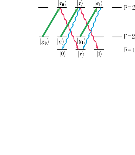
FIG. 2.: The relevant level structures and transitions of atom 1 and atom 2. The two atoms are identical alkali atoms, for example ⁸⁷Rb, but involve different atomic levels. Atom 1 exploits $\left|g_{0}\right\rangle$, $\left|g_{1}\right\rangle$, $\left|e_{0}\right\rangle$, $\left|e_{1}\right\rangle$, and $\left|r\right\rangle$, while atom 2 exploits $\left|g\right\rangle$, $\left|e\right\rangle$, $\left|0\right\rangle$, and $\left|1\right\rangle$. The states $\left|g_{0}\right\rangle$, $\left|g_{1}\right\rangle$, $\left|g\right\rangle$ ($\left|r\right\rangle$, $\left|0\right\rangle$, $\left|1\right\rangle$) correspond to the Zeeman sublevels of the $F=2$ ($F=1$) ground hyperfine level, and $\left|e_{0}\right\rangle$, $\left|e_{1}\right\rangle$, $\left|e\right\rangle$ correspond to the Zeeman sublevels of the $F=2$ excited hyperfine level.

The level structures of atom 1 and atom 2 are jointly shown in Fig. 2. Such atomic level structures can be achieved in ⁸⁷Rb, so we take ⁸⁷Rb as our choice. The states $\left|g_{0}\right\rangle$, $\left|g_{1}\right\rangle$, $\left|g\right\rangle$, $\left|0\right\rangle$, $\left|1\right\rangle$, and $\left|r\right\rangle$ correspond to $\left|F\right.=2,m=-\left.2\right\rangle$, $\left|F\right.=2,m=\left.0\right\rangle$, $\left|F\right.=2,m=-\left.1\right\rangle$, $\left|F\right.=1,m=-\left.1\right\rangle$, $\left|F\right.=1,m=\left.1\right\rangle$, and $\left|F\right.=1,m=\left.0\right\rangle$ of $5S_{1/2}$, respectively. $\left|e_{0}\right\rangle$, $\left|e_{1}\right\rangle$, and $\left|e\right\rangle$ correspond to $\left|F\right.=2,m=-\left.1\right\rangle$, $\left|F\right.=2,m=\left.1\right\rangle$, and $\left|F\right.=2,m=\left.0\right\rangle$ of $5P_{1/2}$, respectively. The qubit of Alice (atom 1) is encoded in $\left|g_{0}\right\rangle$ and $\left|g_{1}\right\rangle$, while the qubit of Bob (atom 2) is encoded in $\left|0\right\rangle$ and $\left|1\right\rangle$. The transitions $\left|g_{0}\right\rangle\rightarrow\left|e_{0}\right\rangle$, $\left|g_{1}\right\rangle\rightarrow\left|e_{1}\right\rangle$ and $\left|g\right\rangle\rightarrow\left|e\right\rangle$ are driven resonantly and adiabatically by right-circularly polarized classical laser pulses, with the corresponding Rabi frequencies signified by $\Omega_{0}(t)$, $\Omega_{1}(t)$ and $\Omega_{2}(t)$ respectively. The transitions $\left|e_{0}\right\rangle\rightarrow\left|r\right\rangle$ and $\left|e\right\rangle\rightarrow\left|1\right\rangle$ ($\left|e_{1}\right\rangle\rightarrow\left|r\right\rangle$ and $\left|e\right\rangle\rightarrow\left|0\right\rangle$) are resonantly coupled to the cavity mode $a_{L}$ ($a_{R}$) with left-circularly (right-circularly) polarization. Because of the symmetry of the atomic level structures, the coupling rates corresponding to $\left|e_{0}\right\rangle\rightarrow\left|r\right\rangle$ and $\left|e_{1}\right\rangle\rightarrow\left|r\right\rangle$ can be simultaneously denoted by $g_{1}$, while those corresponding to $\left|e\right\rangle\rightarrow\left|0\right\rangle$ and $\left|e\right\rangle\rightarrow\left|1\right\rangle$ can be simultaneously denoted by $g_{2}$. Without loss of generality, all the Rabi frequencies and coupling rates are assumed to be real.

III the teleportation scheme

The arbitrary unknown state of atom 1 that is to be transferred from Alice to Bob can be written as

$$\left|\psi\right\rangle_{1}=a\left|g_{0}\right\rangle_{1}+b\left|g_{1}\right\rangle_{1},$$ (1)

where $a$ and $b$ are complex probability amplitudes, and $\left|a\right|^{2}+\left|b\right|^{2}=1$. With cavity A prepared in the vacuum state $\left|0\right\rangle_{A}$, the initial state of the whole system of Alice is $(a\left|g_{0}\right\rangle_{1}+b\left|g_{1}\right\rangle_{1})\left|0\right\rangle_{A}$. If the transitions $\left|g_{0}\right\rangle\rightarrow\left|e_{0}\right\rangle$ and $\left|g_{1}\right\rangle\rightarrow\left|e_{1}\right\rangle$ are driven adiabatically by laser pulse collinear with the cavity axis, atom 1 will be transferred with probability $P_{1}\approx 1$ to the state $\left|r\right\rangle_{1}$ by emitting a photon from the transition $\left|e_{0}\right\rangle\rightarrow\left|r\right\rangle$ or $\left|e_{1}\right\rangle\rightarrow\left|r\right\rangle$. The Hamiltonian of Alice’s system in the rotating frame is given by (assuming $\hbar=1$)

$$H_{1} = i\Omega_{0}(t)(A_{0}-A_{0}^{\dagger})+i\Omega_{1}(t)(A_{1}-A_{1}^{\dagger})-$$ ()

$$ig_{1}(a_{L}^{A\dagger}A_{L}^{A}-A_{L}^{A\dagger}a_{L}^{A})-ig_{1}(a_{R}^{A\dagger}A_{R}^{A}-A_{R}^{A\dagger}a_{R}^{A}),$$

where $A_{0}=\left|g_{0}\right\rangle_{1}\left\langle e_{0}\right|$, $A_{1}=\left|g_{1}\right\rangle_{1}\left\langle e_{1}\right|$, $A_{L}^{A}=\left|r\right\rangle_{1}\left\langle e_{0}\right|$, $A_{R}^{A}=\left|r\right\rangle_{1}\left\langle e_{1}\right|$, and $a_{L}^{A}$ ($a_{R}^{A}$) represents the annihilation operator for the left-circularly (right-circularly) polarized mode of cavity A. The Hamiltonian $H_{1}$ has two orthogonal dark states:

$$\left|D_{0}\right\rangle=\frac{g_{1}\left|g_{0}\right\rangle_{1}\left|0\right\rangle_{A}+\Omega_{0}(t)\left|r\right\rangle_{1}\left|L\right\rangle_{A}}{\sqrt{g_{1}^{2}+\Omega_{0}^{2}(t)}},$$ (3)

and

$$\left|D_{1}\right\rangle=\frac{g_{1}\left|g_{1}\right\rangle_{1}\left|0\right\rangle_{A}+\Omega_{1}(t)\left|r\right\rangle_{1}\left|R\right\rangle_{A}}{\sqrt{g_{1}^{2}+\Omega_{1}^{2}(t)}}.$$ (4)

Under the adiabatic approximation, the state of Alice’s system at time $t$ has the form

$$\left|\Psi(t)\right\rangle_{1A}=ae^{i\varphi_{0}(t)}\left|D_{0}\right\rangle+be^{i\varphi_{1}(t)}\left|D_{1}\right\rangle,$$ (5)

with

$$\varphi_{k}(t)=i\int_{0}^{t}d\tau\left\langle D_{k}\right|\frac{\partial}{\partial\tau}\left|D_{k}\right\rangle-\int_{0}^{t}d\tau E_{k}(\tau),$$ (6)

where $k=0,1$, and $E_{k}(t)$ is the corresponding energy eigenvalue. Here, we have $E_{0}(t)=E_{1}(t)=0$. In Equation (6), the first term on the right side is the adiabatic phase or so-called Berry phase, and the second term is the dynamical phase. Obviously, we have $\varphi_{0}(t)=\varphi_{1}(t)=0$, so $\left|\Psi(t)\right\rangle_{1A}$ becomes

$$\left|\Psi(t)\right\rangle_{1A} = a\left|D_{0}\right\rangle+b\left|D_{1}\right\rangle$$ (7)

$$= (a\cos\theta_{0}(t)\left|g_{0}\right\rangle_{1}+b\cos\theta_{1}(t)\left|g_{1}\right\rangle_{1})\left|0\right\rangle_{A}$$ ()

$$+\left|r\right\rangle_{1}(a\sin\theta_{0}(t)\left|L\right\rangle_{A}+b\sin\theta_{1}(t)\left|R\right\rangle_{A}),$$

with

$$\cos\theta_{i}(t)=g_{1}/\sqrt{g_{1}^{2}+\Omega_{i}^{2}(t)},$$ (9)

and

$$\sin\theta_{i}(t)=\Omega_{i}(t)/\sqrt{g_{1}^{2}+\Omega_{i}^{2}(t)},$$ (10)

where $i=0,1$. The initial state $(a\left|g_{0}\right\rangle_{1}+b\left|g_{1}\right\rangle_{1})\left|0\right\rangle_{A}$ finally evolves into $\left|r\right\rangle_{1}(a\left|L\right\rangle_{A}+b\left|R\right\rangle_{A})$ with $\Omega_{i}(t)$ increasing gradually.

At the same time, Bob switches on a similar laser pulse, which drives the transition $\left|g\right\rangle\rightarrow\left|e\right\rangle$ adiabatically. With cavity B also prepared in the vacuum state $\left|0\right\rangle_{B}$, atom 2, initially prepared in $\left|g\right\rangle_{2}$, will be transferred with probability $P_{2}\approx 1$ to the states $\left|0\right\rangle_{2}$ and $\left|1\right\rangle_{2}$ by emitting a photon from the transition $\left|e\right\rangle\rightarrow\left|0\right\rangle$ or $\left|e\right\rangle\rightarrow\left|1\right\rangle$. The Hamiltonian of Bob’s system in the rotating frame is given by

$$H_{2} = i\Omega_{2}(t)(A_{2}-A_{2}^{\dagger})-ig_{2}(a_{L}^{B\dagger}A_{L}^{B}-A_{L}^{B\dagger}a_{L}^{B})$$ ()

$$-ig_{2}(a_{R}^{B\dagger}A_{R}^{B}-A_{R}^{B\dagger}a_{R}^{B}),$$

where $A_{2}=\left|g\right\rangle_{2}\left\langle e\right|$, $A_{L}^{B}=\left|1\right\rangle_{2}\left\langle e\right|$, $A_{R}^{B}=\left|0\right\rangle_{2}\left\langle e\right|$, and $a_{L}^{B}$ ($a_{R}^{B}$) represents the annihilation operator for the left-circularly (right-circularly) polarized mode of cavity B. The Hamiltonian $H_{2}$ has a dark state:

$$\left|D_{2}\right\rangle=\frac{\sqrt{2}g_{2}\left|g\right\rangle_{2}\left|0\right\rangle_{B}+\Omega_{2}(t)\frac{\left|0\right\rangle_{2}\left|R\right\rangle_{B}+\left|1\right\rangle_{2}\left|L\right\rangle_{B}}{\sqrt{2}}}{\sqrt{2g_{2}^{2}+\Omega_{2}^{2}(t)}}.$$ (12)

Under the adiabatic approximation, the state of Bob’s system at time $t$ has the form

$$\left|\Phi(t)\right\rangle_{2B} = \cos\theta_{2}(t)\left|g\right\rangle_{2}\left|0\right\rangle_{B}$$ ()

$$+\sin\theta_{2}(t)(\left|0\right\rangle_{2}\left|R\right\rangle_{B}+\left|1\right\rangle_{2}\left|L\right\rangle_{B})/\sqrt{2},$$

with

$$\cos\theta_{2}(t)=\sqrt{2}g_{2}/\sqrt{2g_{2}^{2}+\Omega_{2}^{2}(t)},$$ (14)

and

$$\sin\theta_{2}(t)=\Omega_{2}(t)/\sqrt{2g_{2}^{2}+\Omega_{2}^{2}(t)}.$$ (15)

The initial state $\left|0\right\rangle_{B}\left|g\right\rangle_{2}$ finally evolves into $(\left|0\right\rangle_{2}\left|R\right\rangle_{B}+\left|1\right\rangle_{2}\left|L\right\rangle_{B})/\sqrt{2}$ with $\Omega_{2}(t)$ increasing gradually.

Because of the imperfection of the cavities, the two emitted photons will leak out from them and interfere at the device for BSM. Although the complete BSM has been realized successfully in experiment[3], it is inefficient since nonlinear processes are involved. Several mostly used BSMs are based on linear optical elements, and only succeed in $50\%$ or smaller of all the cases. The BSM of our scheme, which has a success probability of the upper bound $50\%$, is shown in Fig. 3 (see Ref.[19]). A straightforward analysis shows that, with the BSM successfully completed on $\left|r\right\rangle_{1}(a\left|L\right\rangle_{A}+b\left|R\right\rangle_{A})(\left|0\right\rangle_{2}\left|R\right\rangle_{B}+\left|1\right\rangle_{2}\left|L\right\rangle_{B})/\sqrt{2}$, which is the joint state of Alice’s and Bob’s systems, the state of atom 2 becomes $a\left|0\right\rangle_{2}\pm b\left|1\right\rangle_{2}$. Concretely, if $D_{1,4}$ or $D_{2,3}$ ($D_{1,3}$ or $D_{2,4}$) are triggered, atom 2 will be on the state $a\left|0\right\rangle_{2}+b\left|1\right\rangle_{2}$ ($a\left|0\right\rangle_{2}-b\left|1\right\rangle_{2}$). Otherwise, the teleportation fails. After Alice has sent the result of the response of the detectors to Bob, he performs an appropriate unitary operation on atom 2, and the teleportation is thus finished.

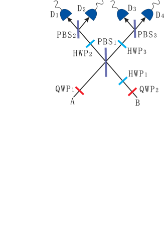
FIG. 3.: The device for Bell state measurement. $PBS_{1,2,3}$ denote polarization beam splitters, $QWP_{1,2}$ signify quarter wave plates, and $D_{1,2,3,4}$ represent detectors. $HWP_{1}$ is a $90^{\circ}$ half wave plate, while $HWP_{2,3}$ are $45^{\circ}$ half wave plates.

In addition, we briefly consider the preparation of the initial state $a\left|g_{0}\right\rangle_{1}+b\left|g_{1}\right\rangle_{1}$ in the experimental demonstration. In Ref.[18], a method is proposed by Law and Eberly to prepare an arbitrarily prescribed superposition of internal Zeeman levels of an atom by Raman pulses. If we apply this method, the initial state can be easily generated. For example, we assume that atom 1 would be firstly prepared in the state $\left|g_{0}\right\rangle_{1}$ by optical pumping. Fig. 4 shows the pulse sequence to generate the initial state $a\left|g_{0}\right\rangle_{1}+b\left|g_{1}\right\rangle_{1}$. Step (1) forces the state $\left|g_{0}\right\rangle_{1}$ to evolve into $a\left|g_{0}\right\rangle_{1}+b\left|0\right\rangle_{1}$. In this step, the area of the Raman pulse should be adjusted according to the CG coefficients and the complex probability amplitudes $a$ and $b$. Step (2) completely transfers the occupation of the state $\left|0\right\rangle_{1}$ to that of the state $\left|g_{1}\right\rangle_{1}$, and thus the state of atom 1 becomes $a\left|g_{0}\right\rangle_{1}+b\left|g_{1}\right\rangle_{1}$. In this step, the required Raman pulse is a $\pi$ pulse.

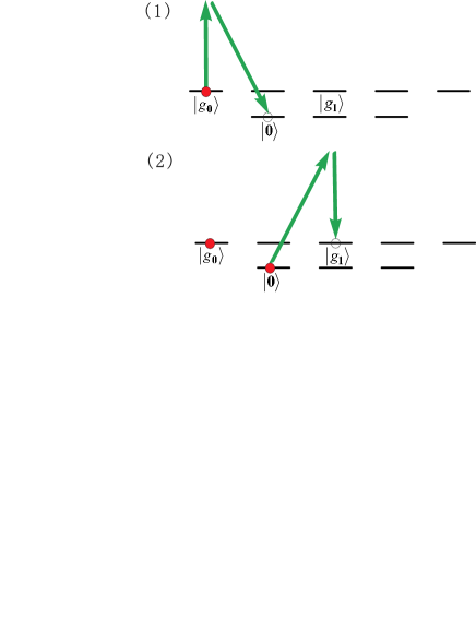
FIG. 4.: A 2-pulse sequence to prepare the initial state $a\left|g_{0}\right\rangle_{1}+b\left|g_{1}\right\rangle_{1}$. The solid circles represent the occupied states, while the empty circles represent the states to be occupied.

IV discussion on the fidelity and advantages of the scheme

Now we turn to the estimation of the fidelity. The BSM does a perfect job only when the output pulse shapes of the two photons match exactly, however, this condition can not be satisfied in our scheme. Approximately, the pulse shape of Bob’s photon[9] is analytically given by

$$f_{B}(t)=\sqrt{\kappa}\sin\theta_{2}(t)\exp[-(\kappa/2)\int_{0}^{t}\sin^{2}\theta_{2}(\tau)d\tau],$$ (16)

where $\kappa$ represents the common decay rate of cavity A and B. The pulse shape of Alice’s photon $f_{A}(t)$ alters with the initial state of atom 1. For special case $\left|\psi\right\rangle_{1}=\left|g_{i}\right\rangle_{1}$ ($i=0,1$), we have

$$f_{Ai}(t)=\sqrt{\kappa}\sin\theta_{i}(t)\exp[-(\kappa/2)\int_{0}^{t}\sin^{2}\theta_{i}(\tau)d\tau],$$ (17)

where $f_{Ai}(t)$ is the corresponding pulse shape. For general case, $f_{A}(t)$ varies from $f_{A0}(t)$ to $f_{A1}(t)$. Therefore the fidelity of our teleportation is highly determined by the difference $\delta$ between $f_{A0}(t)$ and $f_{A1}(t)$. Because

$$\sin\theta_{i}(t) = \Omega_{i}(t)/\sqrt{g_{1}^{2}+\Omega_{i}^{2}(t)}$$ (18)

$$= C_{\Omega_{i}}\widetilde{E}_{1}(t)/\sqrt{C_{g_{1}}^{2}+C_{\Omega_{i}}^{2}\widetilde{E}_{1}^{2}(t)},$$ ()

where $\widetilde{E}_{1}(t)$ is proportional to the slowly-varying amplitude of Alice’s driving pulse by a constant $R$, $\delta$ is entirely generated by the inequality of $C_{\Omega_{i}}$. Here, $C_{\Omega_{0}}=\sqrt{1/3}$ and $C_{\Omega_{1}}=\sqrt{1/2}$. Fortunately, if we choose an appropriate driving pulse shape, $\delta$ can be small enough to be neglected. An example is shown in Fig. 5, where, and in the following, the pulse shape functions are renormalized according to $\int_{0}^{T}f^{2}(t)dt=1$ ($T$ is the driving pulse duration) for convenience of comparison. The two curves overlap very well, and with $\delta$ quantified through $\delta=1-\int_{0}^{T}f_{A0}(t)f_{A1}(t)dt$, we obtain $1-\delta=0.992$. Because

$$\sin\theta_{2}(t) = \Omega_{2}(t)/\sqrt{2g_{2}^{2}+\Omega_{2}^{2}(t)}$$ (19)

$$= C_{\Omega_{2}}\widetilde{E}_{2}(t)/\sqrt{2C_{g_{2}}^{2}+C_{\Omega_{2}}^{2}\widetilde{E}_{2}^{2}(t)},$$ ()

where $\widetilde{E}_{2}(t)$ is proportional to the slowly-varying amplitude of Bob’s driving pulse by a constant $R$, when $\widetilde{E}_{2}(t)$ is chosen to satisfy

$$\widetilde{E}_{2}(t)=(\sqrt{2}C_{g_{2}}C_{\Omega_{1}}/C_{g_{1}}C_{\Omega_{2}})\widetilde{E}_{1}(t)=\sqrt{2/3}\widetilde{E}_{1}(t),$$ (20)

we have $f_{B}(t)=f_{A1}(t)$. The state-dependent fidelity $F$ of the final state of atom 2 with respect to the initial state of atom 1 has the following form

$$F=\sqrt{\left|a\right|^{4}+\left|b\right|^{4}+2\left|a\right|^{2}\left|b\right|^{2}\left(\int_{0}^{T}f_{A}(t)f_{B}(t)dt\right)^{2}}.$$ (21)

Then it is straightforward that $F\gtrsim 1-\delta$ for arbitrary state, so we almost have a fidelity of unity. Furthermore, as the inequality of $C_{\Omega_{i}}$ does not result in the large $\delta$ and thus the large loss in the fidelity, our scheme has another favorable feature. Reasonable as it seems, the fidelity is insensitive to the ratio $\widetilde{E}_{2}(t)/\widetilde{E}_{1}(t)$, with $\widetilde{E}_{1}(t)$ and $\widetilde{E}_{2}(t)$ sharing the same normalized driving pulse shape. So $\widetilde{E}_{2}(t)/\widetilde{E}_{1}(t)$ is not required to equal $\sqrt{2/3}$ accurately.

FIG. 5.: The pulse shape functions $f_{A0}(t)$ (solid curve) and $f_{A1}(t)$ (dashed curve). To satisfy the adiabatic condition, we have taken the driving pulse duration $T=40/\kappa$. $\widetilde{E}_{1}(t)$ is in a Gaussian shape with the peak at $t=T/2$ and the width $t_{w}=\sqrt{2}T/10$, and $E_{1m}=C_{g_{1}}/$ $C_{\Omega_{0}}$, where $E_{1m}$ is the maximum of $\widetilde{E}_{1}(t)$.

A presentation of the advantages of our scheme is now in order. First, our scheme has a high fidelity, with a large success probability of $50\%$ achieved in the ideal case. As shown above, if the driving pulses are chosen appropriately, the fidelity can be made higher than $0.99$ for arbitrary state, and thus approaches unity approximately. Second, our scheme is intrinsically robust to spontaneous emission. This atomic decay is highly suppressed by the adiabatic method, and it only results in the loss of photons even if it happens. Third, compared with the original scheme[7], our scheme also has inherent robustness to output coupling inefficiency of the cavities, transmission loss, and detector inefficiency. In our scheme, all these practical noises and technical imperfections only lead to the loss of photons, and thus loss of the success probability, but have no influence on the fidelity. Whereas in the original scheme, distinguishing between one and two photons is required, so the decrease of the fidelity is inevitable. Besides, the fidelity is insensitive to the ratio of the slowly-varying amplitudes of the driving pulses $\widetilde{E}_{2}(t)/\widetilde{E}_{1}(t)$. This feature removes the requirement to accurately control the intensity of the laser pulse. Finally, our scheme successfully overcomes the experimental difficulties caused by the randomness of the coupling rate. The Lamb-Dicke condition is no longer needed to be satisfied. A far-off resonance trapping (FORT) beam[13, 14, 15] forms many potential wells along the cavity axis, and the bottoms of different potential wells have different coupling rates. In current experiments, one can not control and even does not know precisely in which well the atom is trapped. But in our scheme this kind of uncertainty of the coupling rate is well conquered. So our scheme of teleportation is expected to be implemented with the current cavity QED experimental technology of trapping and manipulating single atoms.

In comparison with the recent similar teleportation scheme[16], our scheme is more robust to the randomness in the atom’s position. First, we do not need each atom to be trapped in the same FORT potential well, and even we need no information on which well the atom is trapped in. Second, the thermal oscillation of the atom, which should be considered when the Lamb-Dicke condition is not satisfied, has no influence on the fidelity of our scheme. Thus the fidelity of our scheme is not random, and is determined with the driving pulses chosen. Furthermore, our scheme wins an advantage over that of Ref.[16] on the high fidelity. Affected by the thermal oscillation of the atom and the randomness on which well the atom is trapped in, the average fidelity of the scheme in Ref.[16] is not as high as that of our scheme.

V conclusion

In summary, we have presented a scheme to teleport the internal state of an atom trapped in a cavity to another atom trapped in a distant cavity by measuring interference of polarized photons through single-photon detectors. Our scheme has a high fidelity of almost unity and a large success probability. Compared with the original scheme, it has several advantages including intrinsic robustness to detection inefficiency and randomness in the atom’s position, and thus well fit the status of the current experiment technology.

REFERENCES

- [1] C.H. Bennett, G. Brassard, C. Crépeau, R. Jozsa, A. Peres, and W.K. Wootters, Phys. Rev. Lett. 70, 1895 (1993).
- [2] D. Bouwmeester, J.-W. Pan, K. Mattle, M. Eibl, H. Weinfurter, and A. Zeilinger, Nature (London) 390, 575 (1997); D. Boschi, S. Branca, F. De Martini, L. Hardy, and S. Popescu, Phys. Rev. Lett. 80, 1121 (1998).
- [3] Y.-H. Kim, S.P. Kulik, and Y. Shih, Phys.Rev.Lett. 86, 1370 (2001).
- [4] E. Lombardi, F. Sciarrino, S. Popescu, and F. De Martini, Phys.Rev.Lett. 88, 070402 (2002); S. Giacomini, F. Sciarrino, E. Lombardi, and F. De Martini, Phys. Rev. A 66, 030302(R) (2002).
- [5] A. Furusawa, J.L. Sorensen, S.L. Braunstein, C.A. Fuchs, H.J. Kimble, and E.S. Polzik, Science 282, 706 (1998); T.C. Zhang, K.W. Goh, C.W. Chou, P. Lodahl, and H.J. Kimble, Phys. Rev. A 67, 033802 (2003).
- [6] L. Davidovich, N. Zagury, M. Brune, J.M. Raimond, and S. Haroche, Phys. Rev. A 50, R895 (1994); J.I. Cirac and A.S. Parkins, Phys. Rev. A 50, R4441 (1994); M.H.Y. Moussa, Phys. Rev. A 55, R3287 (1997); S.-B. Zheng and G.-C. Guo, Phys. Lett. A 232, 171 (1997).
- [7] S. Bose, P.L. Knight, M.B. Plenio, and V. Vedral, Phys. Rev. Lett. 83, 5158 (1999).
- [8] M.B. Plenio, S.F. Huelga, A. Beige, and P.L. Knight, Phys. Rev. A 59, 2468 (1999); J. Hong and H.-W. Lee, Phys. Rev. Lett. 89, 237901 (2002); X.-L. Feng, Z.-M. Zhang, X.-D. Li, S.-Q. Gong, and Z.-Z. Xu, Phys. Rev. Lett. 90, 217902 (2003);A.S. Sorensen and K. Molmer, Phys. Rev. Lett. 90, 127903 (2003); D.E. Browne, M.B. Plenio, and S.F. Huelga, Phys. Rev. Lett. 91, 067901 (2003).
- [9] L.-M. Duan, A. Kuzmich, and H.J. Kimble, Phys. Rev. A 67, 032305 (2003); L.-M. Duan and H.J. Kimble, Phys. Rev. Lett. 90, 253601 (2003).
- [10] L.-M. Duan, M.D. Lukin, J.I. Cirac, and P. Zoller, Nature 414, 413 (2001); L.-M. Duan, Phys. Rev. Lett. 88, 170402 (2002).
- [11] A. Beige, D. Braun, B. Tregenna, and P.L. Knight, Phys. Rev. Lett. 85, 1762 (2000); J. Pachos and H. Walther, Phys. Rev. Lett. 89, 187903 (2002); X.X. Yi, X.H. Su, and L. You, Phys. Rev. Lett. 90, 097902 (2003); A.S. Sorensen and K. Molmer, Phys. Rev. Lett. 91, 097905 (2003).
- [12] J.I. Cirac, P. Zoller, H.J. Kimble, and H. Mabuchi, Phys. Rev. Lett. 78, 3221 (1997); T. Pellizzari, Phys. Rev. Lett. 79, 5242 (1997); S.J. van Enk, J.I. Cirac, and P. Zoller, Phys. Rev. Lett. 78, 4293 (1997).
- [13] C.J. Hood, M.S. Chapman, T.W. Lynn and H.J. Kimble, Phys.Rev.Lett. 80, 4157 (1998); C.J. Hood, T.W. Lyan, A.C. Doherty, A.S. Parkins, and H.J. Kimble, Science 287, 1447 (2000).
- [14] J. Ye, D.W. Vernooy and H.J. Kimble, Phys.Rev.Lett. 83, 4987 (1999).
- [15] J. McKeever, J.R. Buck, A.D. Boozer, A. Kuzmich, H.-C. Nagerl, D.M. Stamper-Kurn, and H.J. Kimble, Phys.Rev.Lett. 90, 133602 (2003).
- [16] J. Cho and H.-W. Lee, quant-ph/0307197 (2003).
- [17] W. Lange and H.J. Kimble, Phys. Rev. A 61, 063817 (2000).
- [18] C.K. Law and J.H. Eberly, Opt. Express 2, 368 (1998).
- [19] J.-W. Pan and A. Zeilinger, Phys. Rev. A 57, 2208 (1998).