Multilinear Formulas and Skepticism of Quantum Computing

Abstract

Several researchers, including Leonid Levin, Gerard ’t Hooft, and Stephen Wolfram, have argued that quantum mechanics will break down before the factoring of large numbers becomes possible.  If this is true, then there should be a natural set of quantum states that can account for all quantum computing experiments performed to date, but not for Shor’s factoring algorithm.  We investigate as a candidate the set of states expressible by a polynomial number of additions and tensor products.  Using a recent lower bound on multilinear formula size due to Raz, we then show that states arising in quantum error-correction require $n^{\Omega(\log n)}$ additions and tensor products even to approximate, which incidentally yields the first superpolynomial gap between general and multilinear formula size of functions.  More broadly, we introduce a complexity classification of pure quantum states, and prove many basic facts about this classification.  Our goal is to refine vague ideas about a breakdown of quantum mechanics into specific hypotheses that might be experimentally testable in the near future.

1 Introduction

QC of the sort that factors long numbers seems firmly rooted in science fiction … The present attitude would be analogous to, say, Maxwell selling the Daemon of his famous thought experiment as a path to cheaper electricity from heat. —Leonid Levin [35]

Quantum computing presents a dilemma: is it reasonable to study a type of computer that has never been built, and might never be built in one’s lifetime?  Some researchers strongly believe the answer is ‘no.’  Their objections generally fall into four categories:

1. There is a fundamental physical reason why large quantum computers can never be built.

2. Even if (A) fails, large quantum computers will never be built in practice.

3. Even if (A) and (B) fail, the speedup offered by quantum computers is of limited theoretical interest.

4. Even if (A), (B), and (C) fail, the speedup is of limited practical value.

The objections can be classified along two axes:

Theoretical Practical

Physical (A) (B)

Algorithmic (C) (D)

  

This paper focuses on objection (A).  Its goal is not to win a debate about this objection, but to lay the groundwork for a rigorous discussion, and thus hopefully lead to new science.  Section 2 provides the philosophical motivation for our paper, by examining the arguments of several quantum computing skeptics, including Leonid Levin, Gerard ’t Hooft, and Stephen Wolfram.  It concludes that a key weakness of their arguments is their failure to answer the following question: Exactly what property separates the quantum states we are sure we can create, from those that suffice for Shor’s factoring algorithm?  We call such a property a Sure/Shor separator.  Section 3 develops a complexity theory of pure quantum states, that studies possible Sure/Shor separators.  In particular, it introduces tree states, which informally are those states $\left|\psi\right\rangle\in\mathcal{H}_{2}^{\otimes n}$ expressible by a polynomial-size ‘tree’ of addition and tensor product gates.  For example, $\alpha\left|0\right\rangle^{\otimes n}+\beta\left|1\right\rangle^{\otimes n}$ and $\left(\alpha\left|0\right\rangle+\beta\left|1\right\rangle\right)^{\otimes n}$ are both tree states.  Section 4 investigates basic properties of this class of states.  Among other results, it shows that any tree state is representable by a tree of polynomial size and logarithmic depth; and that most states do not even have large inner product with any tree state.

Our main results, proved in Section 5, are lower bounds on tree size for various natural families of quantum states.  In particular, Section 5.1 analyzes “subgroup states,” which are uniform superpositions $\left|S\right\rangle$ over all elements of a subgroup $S\leq\mathbb{Z}_{2}^{n}$.  The importance of these states arises from their central role in stabilizer codes, a type of quantum error-correcting code.  We first show that if $S$ is chosen uniformly at random, then with high probability $\left|S\right\rangle$ cannot be represented by any tree of size $n^{o\left(\log n\right)}$.  This result has a corollary of independent complexity-theoretic interest: the first superpolynomial gap between the formula size and the multilinear formula size of a function $f:\left\{0,1\right\}^{n}\rightarrow\mathbb{R}$.  We then present two improvements of our basic lower bound.  First, we show that a random subgroup state cannot even be approximated well in trace distance by any tree of size $n^{o\left(\log n\right)}$.  Second, we “derandomize” the lower bound, by using Reed-Solomon codes to construct an explicit subgroup state with tree size $n^{\Omega\left(\log n\right)}$.

Section 5.2 analyzes the states that arise in Shor’s factoring algorithm—for example, a uniform superposition over all multiples of a fixed positive integer $p$, written in binary.  Originally, we had hoped to show a superpolynomial tree size lower bound for these states as well.  However, we are only able to show such a bound assuming a number-theoretic conjecture.

Our lower bounds use a sophisticated recent technique of Raz [41, 42], which was introduced to show that the permanent and determinant of a matrix require superpolynomial-size multilinear formulas.  Currently, Raz’s technique is only able to show lower bounds of the form $n^{\Omega\left(\log n\right)}$, but we conjecture that $2^{\Omega\left(n\right)}$ lower bounds hold in all of the cases discussed above.

One might wonder how tree size relates to more physical properties of quantum states, such as their robustness to decoherence.  Section 5.3 addresses this question.  In particular, it shows that if $\left|S\right\rangle$ is a superposition over codewords of any sufficiently good erasure code, then $\left|S\right\rangle$ has tree size $n^{\Omega\left(\log n\right)}$, although not vice versa.  It also argues that Raz’s lower bound technique is connected to a notion called “persistence of entanglement,” but gives examples showing that the connection is not exact.

Section 6 addresses the following question.  If the state of a quantum computer at every time step is a tree state, then can the computer be simulated classically?  In other words, letting $\mathsf{TreeBQP}$ be the class of languages accepted by such a machine, does $\mathsf{TreeBQP}=\mathsf{BPP}$?  A positive answer would make tree states more attractive as a Sure/Shor separator.  For once we admit any states incompatible with the polynomial-time Church-Turing thesis, it seems like we might as well go all the way, and admit all states preparable by polynomial-size quantum circuits!  Although we leave this question open, we do show that $\mathsf{TreeBQP}\subseteq\mathsf{\Sigma}_{3}^{\mathsf{P}}\cap\mathsf{\Pi}_{3}^{\mathsf{P}}$, where $\mathsf{\Sigma}_{3}^{\mathsf{P}}\cap\mathsf{\Pi}_{3}^{\mathsf{P}}$ is the third level of the polynomial hierarchy $\mathsf{PH}$.  By contrast, it is conjectured that $\mathsf{BQP}\not\subset\mathsf{PH}$, though admittedly not on strong evidence.

Section 7 discusses the implications of our results for experimental physics.  It advocates a dialectic between theory and experiment, in which theorists would propose a class of quantum states that encompasses everything seen so far, and then experimenters would try to prepare states not in that class.  It also asks whether states with superpolynomial tree size have already been observed in condensed-matter systems; and more broadly, what sort of evidence is needed to establish a state’s existence.  Other issues addressed in Section 7 include how to deal with mixed states and particle position and momentum states, and the experimental relevance of asymptotic bounds.

Finally, two appendices investigate quantum state complexity measures other than tree size.  Appendix 3 shows relationships among tree size, circuit size, bounded-depth tree size, Vidal’s $\chi$ complexity [46], and several other measures.  It also relates questions about quantum state classes to more traditional questions about computational complexity classes.  Appendix 10 studies a weakening of tree size called “manifestly orthogonal tree size,” and shows that this measure can sometimes be characterized exactly, enabling us to prove exponential lower bounds.  Our techniques in Appendix 10 might be of independent interest to complexity theorists.

We conclude in Section 8 with some open problems.

2 How Quantum Mechanics Could Fail

This section discusses objection (A), that quantum computing is impossible for a fundamental physical reason.  Among computer scientists, this objection is most closely associated with Leonid Levin [35].  The following passage captures much of the flavor of his critique:

The major problem [with quantum computing] is the requirement that basic quantum equations hold to multi-hundredth if not millionth decimal positions where the significant digits of the relevant quantum amplitudes reside.  We have never seen a physical law valid to over a dozen decimals.  Typically, every few new decimal places require major rethinking of most basic concepts.  Are quantum amplitudes still complex numbers to such accuracies or do they become quaternions, colored graphs, or sick-humored gremlins? [35]

Among other things, Levin argues that quantum computing is analogous to the unit-cost arithmetic model, and should be rejected for essentially the same reasons; that claims to the contrary rest on a confusion between metric and topological approximation; that quantum fault-tolerance theorems depend on extravagant assumptions; and that even if a quantum computer failed, we could not measure its state to prove a breakdown of quantum mechanics, and thus would be unlikely to learn anything new.

A few responses to Levin’s arguments can be offered immediately.  First, even classically, one can flip a coin a thousand times to produce probabilities of order $2^{-1000}$.  Should one dismiss such probabilities as unphysical?  At the very least, it is not obvious that amplitudes should behave differently than probabilities with respect to error—since both evolve linearly, and neither is directly observable.

Second, if Levin believes that quantum mechanics will fail, but is agnostic about what will replace it, then his argument can be turned around.  How do we know that the successor to quantum mechanics will limit us to $\mathsf{BPP}$, rather than letting us solve (say) $\mathsf{PSPACE}$-complete problems?  This is more than a logical point.  Abrams and Lloyd [4] argue that a wide class of nonlinear variants of the Schrödinger equation would allow $\mathsf{NP}$-complete and even $\mathsf{\#P}$-complete problems to be solved in polynomial time.  And Penrose [39], who proposed a model for ‘objective collapse’ of the wavefunction, believes that his proposal takes us outside the set of computable functions entirely!

Third, to falsify quantum mechanics, it would suffice to show that a quantum computer evolved to some state far from the state that quantum mechanics predicts.  Measuring the exact state is unnecessary.  Nobel prizes have been awarded in the past ‘merely’ for falsifying a previously held theory, rather than replacing it by a new one.  An example is the physics Nobel awarded to Fitch [19] and Cronin [17] in 1980 for discovering CP symmetry violation.

Perhaps the key to understanding Levin’s unease about quantum computing lies in his remark that “we have never seen a physical law valid to over a dozen decimals.”  Here he touches on a serious epistemological question: How far should we extrapolate from today’s experiments to where quantum mechanics has never been tested?  We will try to address this question by reviewing the evidence for quantum mechanics.  For our purposes it will not suffice to declare the predictions of quantum mechanics “verified to one part in a trillion,” because we need to distinguish at least three different types of prediction: interference, entanglement, and Schrödinger cats.  Let us consider these in turn.

1. Interference.  If the different paths that an electron could take in its orbit around a nucleus did not interfere destructively, canceling each other out, then electrons would not have quantized energy levels.  So being accelerating electric charges, they would lose energy and spiral into their respective nuclei, and all matter would disintegrate.  That this has not happened—together with the results of (for example) single-photon double-slit experiments—is compelling evidence for the reality of quantum interference.

2. Entanglement.  One might accept that a single particle’s position is described by a wave in three-dimensional phase space, but deny that two particles are described by a wave in six-dimensional phase space.  However, the Bell inequality experiments of Aspect et al. [8] and successors have convinced all but a few physicists that quantum entanglement exists, can be maintained over large distances, and cannot be explained by local hidden-variable theories.

3. Schrödinger Cats.  Accepting two- and three-particle entanglement is not the same as accepting that whole molecules, cats, humans, and galaxies can be in coherent superposition states.  However, recently Arndt et al. [7] have performed the double-slit interference experiment using $C_{60}$ molecules (buckyballs) instead of photons; while Friedman et al. [20] have found evidence that a superconducting current, consisting of billions of electrons, can enter a coherent superposition of flowing clockwise around a coil and flowing counterclockwise (see Leggett [34] for a survey of such experiments).  Though short of cats, these experiments at least allow us to say the following: if we could build a general-purpose quantum computer with as many components as have already been placed into coherent superposition, then on certain problems, that computer would outperform any computer in the world today.

Having reviewed some of the evidence for quantum mechanics, we must now ask what alternatives have been proposed that might also explain the evidence.  The simplest alternatives are those in which quantum states “spontaneously collapse” with some probability, as in the GRW (Ghirardi-Rimini-Weber) theory [23].  The drawbacks of the GRW theory include violations of energy conservation, and parameters that must be fine-tuned to avoid conflicting with experiments.  More relevant for us, though, is that the collapses postulated by the theory are only in the position basis, so that quantum information stored in internal degrees of freedom (such as spin) is unaffected.  Furthermore, even if we extended the theory to collapse those internal degrees, large quantum computers could still be built.  For the theory predicts roughly one collapse per particle per $10^{15}$ seconds, with a collapse affecting everything in a $10^{-7}$-meter vicinity.  So even in such a vicinity, one could perform a computation involving (say) $10^{10}$ particles for $10^{5}$ seconds.  Finally, as pointed out to us by Rob Spekkens, standard quantum error-correction techniques might be used to overcome even GRW-type decoherence.

A second class of alternatives includes those of ’t Hooft [30] and Wolfram [48], in which something like a deterministic cellular automaton underlies quantum mechanics.  On the basis of his theory, ’t Hooft predicts that “[i]t will never be possible to construct a ‘quantum computer’ that can factor a large number faster, and within a smaller region of space, than a classical machine would do, if the latter could be built out of parts at least as large and as slow as the Planckian dimensions” [30].  Similarly, Wolfram states that “[i]ndeed within the usual formalism [of quantum mechanics] one can construct quantum computers that may be able to solve at least a few specific problems exponentially faster than ordinary Turing machines.  But particularly after my discoveries … I strongly suspect that even if this is formally the case, it will still not turn out to be a true representation of ultimate physical reality, but will instead just be found to reflect various idealizations made in the models used so far” [48, p.771].

The obvious question then is how these theories account for Bell inequality violations.  We confess to being unable to understand ’t Hooft’s answer to this question, except that he believes that the usual notions of causality and locality might no longer apply in quantum gravity.  As for Wolfram’s theory, which involves “long-range threads” to account for Bell inequality violations, we argued in [1] that it fails Wolfram’s own desiderata of causal and relativistic invariance.

So the challenge for quantum computing skeptics is clear.  Ideally, come up with an alternative to quantum mechanics—even an idealized toy theory—that can account for all present-day experiments, yet would not allow large-scale quantum computation.  Failing that, at least say what you take quantum mechanics’ domain of validity to be.  One way to do this would be to propose a set $S$ of quantum states that you believe corresponds to possible physical states of affairs.  The set $S$ must contain all “Sure states” (informally, the states that have already been demonstrated in the lab), but no “Shor states” (again informally, the states that can be shown to suffice for factoring, say, $500$-digit numbers).  If $S$ satisfies both of these constraints, then we call $S$ a Sure/Shor separator (see Figure 1).

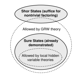
Figure 1: A Sure/Shor separator must contain all Sure states but no Shor states.  That is why neither local hidden variables nor the GRW theory yields a Sure/Shor separator.

Of course, an alternative theory need not involve a sharp cutoff between possible and impossible states.  So it is perfectly acceptable for a skeptic to define a “complexity measure” $C\left(\left|\psi\right\rangle\right)$ for quantum states, and then say something like the following:  If $\left|\psi_{n}\right\rangle$ is a state of $n$ spins, and $C\left(\left|\psi_{n}\right\rangle\right)$ is at most, say, $n^{2}$, then I predict that $\left|\psi_{n}\right\rangle$ can be prepared using only “polynomial effort.”  Also, once prepared, $\left|\psi_{n}\right\rangle$ will be governed by standard quantum mechanics to extremely high precision.  All states created to date have had small values of $C\left(\left|\psi_{n}\right\rangle\right)$.  However, if $C\left(\left|\psi_{n}\right\rangle\right)$ grows as, say, $2^{n}$, then I predict that $\left|\psi_{n}\right\rangle$ requires “exponential effort” to prepare, or else is not even approximately governed by quantum mechanics, or else does not even make sense in the context of an alternative theory.  The states that arise in Shor’s factoring algorithm have exponential values of $C\left(\left|\psi_{n}\right\rangle\right)$.  So as my Sure/Shor separator, I propose the set of all infinite families of states $\left\{\left|\psi_{n}\right\rangle\right\}_{n\geq 1}$, where $\left|\psi_{n}\right\rangle$ has $n$ qubits, such that $C\left(\left|\psi_{n}\right\rangle\right)\leq p\left(n\right)$ for some polynomial $p$.

To understand the importance of Sure/Shor separators, it is helpful to think through some examples.  A major theme of Levin’s arguments was that exponentially small amplitudes are somehow unphysical.  However, clearly we cannot reject all states with tiny amplitudes—for would anyone dispute that the state $2^{-5000}\left(\left|0\right\rangle+\left|1\right\rangle\right)^{\otimes 10000}$ is formed whenever $10,000$ photons are each polarized at $45^{\circ}$?  Indeed, once we accept $\left|\psi\right\rangle$ and $\left|\varphi\right\rangle$ as Sure states, we are almost forced to accept $\left|\psi\right\rangle\otimes\left|\varphi\right\rangle$ as well—since we can imagine, if we like, that $\left|\psi\right\rangle$ and $\left|\varphi\right\rangle$ are prepared in two separate laboratories.  So considering a Shor state such as

$$\left|\Phi\right\rangle=\frac{1}{2^{n/2}}\sum_{r=0}^{2^{n}-1}\left|r\right\rangle\left|x^{r}\operatorname{mod}N\right\rangle,$$

what property of this state could quantum computing skeptics latch onto as being physically extravagant?  They might complain that $\left|\Phi\right\rangle$ involves entanglement across hundreds or thousands of particles; but as mentioned earlier, there are other states with that same property, namely the “Schrödinger cats” $\left(\left|0\right\rangle^{\otimes n}+\left|1\right\rangle^{\otimes n}\right)/\sqrt{2}$, that should be regarded as Sure states.  Alternatively, the skeptics might object to the combination of exponentially small amplitudes with entanglement across hundreds of particles.  However, simply viewing a Schrödinger cat state in the Hadamard basis produces an equal superposition over all strings of even parity, which has both properties.  We seem to be on a slippery slope leading to all of quantum mechanics!  Is there any defensible place to draw a line?

The dilemma above is what led us to propose tree states as a possible Sure/Shor separator.  The idea, which might seem more natural to logicians than to physicists, is this.  Once we accept the linear combination and tensor product rules of quantum mechanics—allowing $\alpha\left|\psi\right\rangle+\beta\left|\varphi\right\rangle$ and $\left|\psi\right\rangle\otimes\left|\varphi\right\rangle$ into our set $S$ of possible states whenever $\left|\psi\right\rangle,\left|\varphi\right\rangle\in S$—one of our few remaining hopes for keeping $S$ a proper subset of the set of all states is to impose some restriction on how those two rules can be iteratively applied.  In particular, we could let $S$ be the closure of $\left\{\left|0\right\rangle,\left|1\right\rangle\right\}$ under a polynomial number of linear combinations and tensor products.  That is, $S$ is the set of all infinite families of states $\left\{\left|\psi_{n}\right\rangle\right\}_{n\geq 1}$ with $\left|\psi_{n}\right\rangle\in\mathcal{H}_{2}^{\otimes n}$, such that $\left|\psi_{n}\right\rangle$ can be expressed as a “tree” involving at most $p\left(n\right)$ addition, tensor product, $\left|0\right\rangle$, and $\left|1\right\rangle$ gates for some polynomial $p$ (see Figure 2).

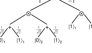
Figure 2: Expressing $\left(\left|00\right\rangle+\left|01\right\rangle+\left|10\right\rangle-\left|11\right\rangle\right)/2$ by a tree of linear combination and tensor product gates, with scalar multiplication along edges.  Subscripts denote the identity of a qubit.

To be clear, we are not advocating that “all states in Nature are tree states” as a serious physical hypothesis.  Indeed, even if we believed firmly in a breakdown of quantum mechanics, there are other choices for the set $S$ that seem equally reasonable.  For example, define orthogonal tree states similarly to tree states, except that we can only form the linear combination $\alpha\left|\psi\right\rangle+\beta\left|\varphi\right\rangle$ if $\left\langle\psi|\varphi\right\rangle=0$.  Rather than choose among tree states, orthogonal tree states, and the other candidate Sure/Shor separators that occurred to us, our approach will be to prove everything we can about all of them.  If we devote more space to tree states than to others, that is simply because tree states are the subject of our most interesting results.  On the other hand, if we show (for example) that $\left\{\left|\psi_{n}\right\rangle\right\}$ is not a tree state, then we have also shown that $\left\{\left|\psi_{n}\right\rangle\right\}$ is not an orthogonal tree state.  So many candidate separators are related to each other; and indeed, their relationships will be a major theme of the paper.

Let us summarize.  To debate whether quantum computing is fundamentally impossible, we need at least one proposal for how it could be impossible.  Since even skeptics admit that quantum mechanics is valid within some “regime,” a key challenge for any such proposal is to separate the regime of acknowledged validity from the quantum computing regime.  Though others will disagree, we do not see any choice but to identify those two regimes with classes of quantum states.  For gates and measurements that suffice for quantum computing have already been demonstrated experimentally.  Thus, if we tried to identify the two regimes with classes of gates or measurements, then we could equally well talk about the class of states on which all $1$- and $2$-qubit operations behave as expected.  A similar argument would apply if we identified the two regimes with classes of quantum circuits—since any “memory” that a quantum system retains of the previous gates in a circuit, is part of the system’s state by definition.  So: states, gates, measurements, circuits—what else is there?

We should stress that none of the above depends on the interpretation of quantum mechanics.  In particular, it is irrelevant whether we regard quantum states as “really out there” or as representing subjective knowledge—since in either case, the question is whether there can exist systems that we would describe by $\left|\psi\right\rangle$ based on their observed behavior.

Once we agree to seek a Sure/Shor separator, we quickly find that the obvious ideas—based on precision in amplitudes, or entanglement across of hundreds of particles—are nonstarters.  The only idea that we have found plausible is to limit the class of allowed quantum states to those with some kind of succinct representation.  That still leaves numerous possibilities; and for each one, it might be a difficult problem to decide whether a given $\left|\psi\right\rangle$ is succinctly representable or not.  Thus, constructing a useful theory of Sure/Shor separators will not be easy.  But we should start somewhere.

3 Classifying Quantum States

In both quantum and classical complexity theory, the objects studied are usually sets of languages or Boolean functions.  However, a generic $n$-qubit quantum state requires exponentially many classical bits to describe, and this suggests looking at the complexity of quantum states themselves.  That is, which states have polynomial-size classical descriptions of various kinds?  This question has been studied from several angles by Aharonov and Ta-Shma [5]; Janzing, Wocjan, and Beth [31]; Vidal [46]; and Green et al. [28].  Here we propose a general framework for the question.  For simplicity, we limit ourselves to pure states $\left|\psi_{n}\right\rangle\in\mathcal{H}_{2}^{\otimes n}$ with the fixed orthogonal basis $\left\{\left|x\right\rangle:x\in\left\{0,1\right\}^{n}\right\}$.  Also, by ‘states’ we mean infinite families of states $\left\{\left|\psi_{n}\right\rangle\right\}_{n\geq 1}$.

Like complexity classes, pure quantum states can be organized into a hierarchy (see Figure 3).  At the bottom are the classical basis states, which have the form $\left|x\right\rangle$ for some $x\in\left\{0,1\right\}^{n}$.  We can generalize classical states in two directions: to the class $\mathsf{\otimes}_{\mathsf{1}}$ of separable states, which have the form $\left(\alpha_{1}\left|0\right\rangle+\beta_{1}\left|1\right\rangle\right)\otimes\cdots\otimes\left(\alpha_{n}\left|0\right\rangle+\beta_{n}\left|1\right\rangle\right)$; and to the class $\mathsf{\Sigma}_{\mathsf{1}}$, which consists of all states $\left|\psi_{n}\right\rangle$ that are superpositions of at most $p\left(n\right)$ classical states, where $p$ is a polynomial.  At the next level, $\mathsf{\otimes}_{\mathsf{2}}$ contains the states that can be written as a tensor product of $\mathsf{\Sigma}_{\mathsf{1}}$ states, with qubits permuted arbitrarily.  Likewise, $\mathsf{\Sigma}$₂ contains the states that can be written as a linear combination of a polynomial number of $\mathsf{\otimes}_{\mathsf{1}}$ states.  We can continue indefinitely to $\mathsf{\Sigma}$₃, $\mathsf{\otimes}_{\mathsf{3}}$, etc.  Containing the whole ‘tensor-sum hierarchy’ $\mathsf{\cup}_{\mathsf{k}}\mathsf{\Sigma}$${}_{\mathsf{k}}=\mathsf{\cup}_{\mathsf{k}}\mathsf{\otimes}_{\mathsf{k}}$ is the class $\mathsf{Tree}$, of all states expressible by a polynomial-size tree of additions and tensor products nested arbitrarily.  Formally, $\mathsf{Tree}$ consists of all states $\left|\psi_{n}\right\rangle$ such that $\operatorname*{TS}\left(\left|\psi_{n}\right\rangle\right)\leq p\left(n\right)$ for some polynomial $p$, where the tree size $\operatorname*{TS}\left(\left|\psi_{n}\right\rangle\right)$ is defined as follows.

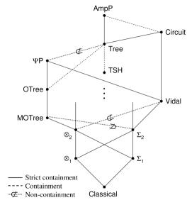
Figure 3: Relations among quantum state classes.

Definition 1

A quantum state tree over $\mathcal{H}_{2}^{\otimes n}$ is a rooted tree where each leaf vertex is labeled with $\alpha\left|0\right\rangle+\beta\left|1\right\rangle$ for some $\alpha,\beta\in\mathsf{C}$, and each non-leaf vertex (called a gate) is labeled with either $+$ or $\otimes$.  Each vertex $v$ is also labeled with a set $S\left(v\right)\subseteq\left\{1,\ldots,n\right\}$, such that

1. If $v$ is a leaf then $\left|S\left(v\right)\right|=1$,

2. If $v$ is the root then $S\left(v\right)=\left\{1,\ldots,n\right\}$,

3. If $v$ is a $+$ gate and $w$ is a child of $v$, then $S\left(w\right)=S\left(v\right)$,

4. If $v$ is a $\otimes$ gate and $w_{1},\ldots,w_{k}$ are the children of $v$, then $S\left(w_{1}\right),\ldots,S\left(w_{k}\right)$ are pairwise disjoint and form a partition of $S\left(v\right)$.

Finally, if $v$ is a $+$ gate, then the outgoing edges of $v$ are labeled with complex numbers.  For each $v$, the subtree rooted at $v$ represents a quantum state of the qubits in $S\left(v\right)$ in the obvious way.  We require this state to be normalized for each $v$.

We say a tree is orthogonal if it satisfies the further condition that if $v$ is a $+$ gate, then any two children $w_{1},w_{2}$ of $v$ represent $\left|\psi_{1}\right\rangle,\left|\psi_{2}\right\rangle$ with $\left\langle\psi_{1}|\psi_{2}\right\rangle=0$.  If the condition $\left\langle\psi_{1}|\psi_{2}\right\rangle=0$ can be replaced by the stronger condition that for all basis states $\left|x\right\rangle$, either $\left\langle\psi_{1}|x\right\rangle=0$ or $\left\langle\psi_{2}|x\right\rangle=0$, then we say the tree is manifestly orthogonal.  Manifest orthogonality is an extremely unphysical definition; we introduce it only because it is interesting from a lower bounds perspective.

For reasons of convenience, we define the size $\left|T\right|$ of a tree $T$ to be the number of leaf vertices.  Then given a state $\left|\psi\right\rangle\in\mathcal{H}_{2}^{\otimes n}$, the tree size $\operatorname*{TS}\left(\left|\psi\right\rangle\right)$ is the minimum size of a tree that represents $\left|\psi\right\rangle$.  The orthogonal tree size $\operatorname*{OTS}\left(\left|\psi\right\rangle\right)$ and manifestly orthogonal tree size $\operatorname*{MOTS}\left(\left|\psi\right\rangle\right)$ are defined similarly.  Then $\mathsf{OTree}$ is the class of $\left|\psi_{n}\right\rangle$ such that $\operatorname*{OTS}\left(\left|\psi_{n}\right\rangle\right)\leq p\left(n\right)$ for some polynomial $p$, and $\mathsf{MOTree}$ is the class such that $\operatorname*{MOTS}\left(\left|\psi_{n}\right\rangle\right)\leq p\left(n\right)$ for some $p$.

It is easy to see that

$$n\leq\operatorname*{TS}\left(\left|\psi\right\rangle\right)\leq\operatorname*{OTS}\left(\left|\psi\right\rangle\right)\leq\operatorname*{MOTS}\left(\left|\psi\right\rangle\right)\leq n2^{n}$$

for every $\left|\psi\right\rangle$, and that the set of $\left|\psi\right\rangle$ such that $\operatorname*{TS}\left(\left|\psi\right\rangle\right)<2^{n}$ has measure $0$ in $\mathcal{H}_{2}^{\otimes n}$.  Two other important properties of $\operatorname*{TS}$ and $\operatorname*{OTS}$ are as follows:

Proposition 2

1. $\operatorname*{TS}$ and $\operatorname*{OTS}$ are invariant under local basis changes, up to a constant factor of $2$.

2. If $\left|\phi\right\rangle$ is obtained from $\left|\psi\right\rangle$ by applying a $k$-qubit unitary, then $\operatorname*{TS}\left(\left|\phi\right\rangle\right)\leq k4^{k}\operatorname*{TS}\left(\left|\psi\right\rangle\right)$ and $\operatorname*{OTS}\left(\left|\phi\right\rangle\right)\leq k4^{k}\operatorname*{OTS}\left(\left|\psi\right\rangle\right)$.

Proof.

1. Simply replace each occurrence of $\left|0\right\rangle$ in the original tree by a tree for $\alpha\left|0\right\rangle+\beta\left|1\right\rangle$, and each occurrence of $\left|1\right\rangle$ by a tree for $\gamma\left|0\right\rangle+\delta\left|1\right\rangle$, as appropriate.

2. Suppose without loss of generality that the gate is applied to the first $k$ qubits.  Let $T$ be a tree representing $\left|\psi\right\rangle$, and let $T_{y}$ be the restriction of $T$ obtained by setting the first $k$ qubits to $y\in\left\{0,1\right\}^{k}$.  Clearly $\left|T_{y}\right|\leq\left|T\right|$.  Furthermore, we can express $\left|\phi\right\rangle$ in the form $\sum_{y\in\left\{0,1\right\}^{k}}S_{y}T_{y}$, where each $S_{y}$ represents a $k$-qubit state and hence is expressible by a tree of size $k2^{k}$.

 

We can also define the $\varepsilon$-approximate tree size $\operatorname*{TS}_{\varepsilon}\left(\left|\psi\right\rangle\right)$ to be the minimum size of a tree representing a state $\left|\varphi\right\rangle$ such that $\left|\left\langle\psi|\varphi\right\rangle\right|^{2}\geq 1-\varepsilon$, and define $\operatorname*{OTS}_{\varepsilon}\left(\left|\psi\right\rangle\right)$ and $\operatorname*{MOTS}_{\varepsilon}\left(\left|\psi\right\rangle\right)$ similarly.

Definition 3

An arithmetic formula (over the ring $\mathbb{C}$ and $n$ variables) is a rooted binary tree where each leaf vertex is labeled with either a complex number or a variable in $\left\{x_{1},\ldots,x_{n}\right\}$, and each non-leaf vertex is labeled with either $+$ or $\times$.  Such a tree represents a polynomial $p\left(x_{1},\ldots,x_{n}\right)$ in the obvious way.  We call a polynomial multilinear if no variable appears raised to a higher power than $1$, and an arithmetic formula multilinear if the polynomials computed by each of its subtrees are multilinear.

The size $\left|\Phi\right|$ of a multilinear formula $\Phi$ is the number of leaf vertices.  Given a multilinear polynomial $p$, the multilinear formula size $\operatorname*{MFS}\left(p\right)$ is the minimum size of a multilinear formula that represents $p$.  Then given a function $f:\left\{0,1\right\}^{n}\rightarrow\mathbb{C}$, we define

$$\operatorname*{MFS}\left(f\right)=\min_{p~{}:~{}p\left(x\right)=f\left(x\right)~{}\forall x\in\left\{0,1\right\}^{n}}\operatorname*{MFS}\left(p\right).$$

(Actually $p$ turns out to be unique [38].)  We can also define the $\varepsilon$-approximate multilinear formula size of $f$,

$$\operatorname*{MFS}\nolimits_{\varepsilon}\left(f\right)=\min_{p~{}:~{}\left\|p-f\right\|_{2}^{2}\leq\varepsilon}\operatorname*{MFS}\left(p\right)$$

where $\left\|p-f\right\|_{2}^{2}=\sum_{x\in\left\{0,1\right\}^{n}}\left|p\left(x\right)-f\left(x\right)\right|^{2}$.  (This metric is closely related to the inner product $\sum_{x}p\left(x\right)^{\ast}f\left(x\right)$, but is often more convenient to work with.)  Now given a state $\left|\psi\right\rangle=\sum_{x\in\left\{0,1\right\}^{n}}\alpha_{x}\left|x\right\rangle$ in $\mathcal{H}_{2}^{\otimes n}$, let $f_{\psi}$ be the function from $\left\{0,1\right\}^{n}$ to $\mathbb{C}$ defined by $f_{\psi}\left(x\right)=\alpha_{x}$.

Theorem 4

For all $\left|\psi\right\rangle$,

1. $\operatorname*{MFS}\left(f_{\psi}\right)=O\left(\operatorname*{TS}\left(\left|\psi\right\rangle\right)\right)$.

2. $\operatorname*{TS}\left(\left|\psi\right\rangle\right)=O\left(\operatorname*{MFS}\left(f_{\psi}\right)+n\right)$.

3. $\operatorname*{MFS}_{\delta}\left(f_{\psi}\right)=O\left(\operatorname*{TS}_{\varepsilon}\left(\left|\psi\right\rangle\right)\right)$ where $\delta=2-2\sqrt{1-\varepsilon}$.

4. $\operatorname*{TS}_{2\varepsilon}\left(\left|\psi\right\rangle\right)=O\left(\operatorname*{MFS}_{\varepsilon}\left(f_{\psi}\right)+n\right)$.

Proof.

1. Given a tree representing $\left|\psi\right\rangle$, replace every unbounded fan-in gate by a collection of binary gates, every $\otimes$ by $\times$, every $\left|1\right\rangle_{i}$ vertex by $x_{i}$, and every $\left|0\right\rangle_{i}$ vertex by a formula for $1-x_{i}$.  Push all multiplications by constants at the edges down to $\times$ gates at the leaves.

2. Given a multilinear formula $\Phi$ for $f_{\psi}$, let $p\left(v\right)$ be the polynomial computed at vertex $v$ of $\Phi$, and let $S\left(v\right)$ be the set of variables that appears in $p\left(v\right)$.  First, call $\Phi$ syntactic if at every $\times$ gate with children $v$ and $w$, $S\left(v\right)\cap S\left(w\right)=\varnothing$.  A lemma of Raz [41] states that we can always make $\Phi$ syntactic without increasing its size.

   Second, at every $+$ gate $u$ with children $v$ and $w$, enlarge both $S\left(v\right)$ and $S\left(w\right)$ to $S\left(v\right)\cup S\left(w\right)$, by multiplying $p\left(v\right)$ by $x_{i}+\left(1-x_{i}\right)$ for every $x_{i}\in S\left(w\right)\setminus S\left(v\right)$, and multiplying $p\left(w\right)$ by $x_{i}+\left(1-x_{i}\right)$ for every $x_{i}\in S\left(v\right)\setminus S\left(w\right)$.  Doing this does not invalidate any $\times$ gate that is an ancestor of $u$, since by the assumption that $\Phi$ is syntactic, $p\left(u\right)$ is never multiplied by any polynomial containing variables in $S\left(v\right)\cup S\left(w\right)$.  Similarly, enlarge $S\left(r\right)$ to $\left\{x_{1},\ldots,x_{n}\right\}$ where $r$ is the root of $\Phi$.

   Third, call $v$ max-linear if $\left|S\left(v\right)\right|=1$ but $\left|S\left(w\right)\right|>1$ where $w$ is the parent of $v$.  If $v$ is max-linear and $p\left(v\right)=a+bx_{i}$, then replace the tree rooted at $v$ by a tree computing $a\left|0\right\rangle_{i}+\left(a+b\right)\left|1\right\rangle_{i}$.  Also, replace all multiplications by constants higher in $\Phi$ by multiplications at the edges.  (Because of the second step, there are no additions by constants higher in $\Phi$.)  Replacing every $\times$ by $\otimes$ then gives a tree representing $\left|\psi\right\rangle$, whose size is easily seen to be $O\left(\left|\Phi\right|+n\right)$ .

3. Apply the reduction from part (i).  Let the resulting multilinear formula compute polynomial $p$; then

   $$\sum_{x\in\left\{0,1\right\}^{n}}\left|p\left(x\right)-f_{\psi}\left(x\right)\right|^{2}=2-2\sum_{x\in\left\{0,1\right\}^{n}}p\left(x\right)\overline{f_{\psi}\left(x\right)}\leq 2-2\sqrt{1-\varepsilon}=\delta.$$

4. Apply the reduction from part (ii).  Let $\left(\beta_{x}\right)_{x\in\left\{0,1\right\}^{n}}$ be the resulting amplitude vector; since this vector might not be normalized, divide each $\beta_{x}$ by $\sum_{x}\left|\beta_{x}\right|^{2}$ to produce $\beta_{x}^{\prime}$.  Then

   $$\left|\sum_{x\in\left\{0,1\right\}^{n}}\beta_{x}^{\prime}\overline{\alpha_{x}}\right|^{2} =1-\frac{1}{2}\sum_{x\in\left\{0,1\right\}^{n}}\left|\beta_{x}^{\prime}-\alpha_{x}\right|^{2}$$

   $$\geq 1-\frac{1}{2}\left(\sqrt{\sum_{x\in\left\{0,1\right\}^{n}}\left|\beta_{x}^{\prime}-\beta_{x}\right|^{2}}+\sqrt{\sum_{x\in\left\{0,1\right\}^{n}}\left|\beta_{x}-\alpha_{x}\right|^{2}}\right)^{2}$$

   $$\geq 1-\frac{1}{2}\left(2\sqrt{\varepsilon}\right)^{2}=1-2\varepsilon.$$

 

Besides $\mathsf{Tree}$, $\mathsf{OTree}$, and $\mathsf{MOTree}$, four other classes of quantum states deserve mention:

$\mathsf{Circuit}$, a circuit analog of $\mathsf{Tree}$, contains the states $\left|\psi_{n}\right\rangle=\sum_{x}\alpha_{x}\left|x\right\rangle$ such that for all $n$, there exists a multilinear arithmetic circuit of size $p\left(n\right)$ over the complex numbers that outputs $\alpha_{x}$ given $x$ as input, for some polynomial $p$.  (Multilinear circuits are the same as multilinear trees, except that they allow unbounded fanout—that is, polynomials computed at intermediate points can be reused arbitrarily many times.)

$\mathsf{AmpP}$ contains the states $\left|\psi_{n}\right\rangle=\sum_{x}\alpha_{x}\left|x\right\rangle$ such that for all $n,b$, there exists a classical circuit of size $p\left(n+b\right)$ that outputs $\alpha_{x}$ to $b$ bits of precision given $x$ as input, for some polynomial $p$.

$\mathsf{Vidal}$ contains the states that are ‘polynomially entangled’ in the sense of Vidal [46].  Given a partition of $\left\{1,\ldots,n\right\}$ into $A$ and $B$, let $\chi_{A}\left(\left|\psi_{n}\right\rangle\right)$ be the minimum $k$ for which $\left|\psi_{n}\right\rangle$ can be written as $\sum_{i=1}^{k}\alpha_{i}\left|\varphi_{i}^{A}\right\rangle\otimes\left|\varphi_{i}^{B}\right\rangle$, where $\left|\varphi_{i}^{A}\right\rangle$ and $\left|\varphi_{i}^{B}\right\rangle$ are states of qubits in $A$ and $B$ respectively.   ($\chi_{A}\left(\left|\psi_{n}\right\rangle\right)$ is known as the Schmidt rank; see [37] for more information.)  Let $\chi\left(\left|\psi_{n}\right\rangle\right)=\max_{A}\chi_{A}\left(\left|\psi_{n}\right\rangle\right)$.  Then $\left|\psi_{n}\right\rangle\in\mathsf{Vidal}$ if and only if $\chi\left(\left|\psi_{n}\right\rangle\right)\leq p\left(n\right)$ for some polynomial $p$.

$\mathsf{\Psi P}$ contains the states $\left|\psi_{n}\right\rangle$ such that for all $n$ and $\varepsilon>0$, there exists a quantum circuit of size $p\left(n+\log\left(1/\varepsilon\right)\right)$ that maps the all-$0$ state to a state some part of which has trace distance at most $1-\varepsilon$ from $\left|\psi_{n}\right\rangle$, for some polynomial $p$.  Because of the Solovay-Kitaev Theorem [32, 37], $\mathsf{\Psi P}$ is invariant under the choice of universal gate set.

4 Basic Results

Before studying the tree size of specific quantum states, we would like to know in general how tree size behaves as a complexity measure.  In this section we prove three rather nice properties of tree size.

Theorem 5

For all $\varepsilon>0$, there exists a tree representing $\left|\psi\right\rangle$ of size $O\left(\operatorname*{TS}\left(\left|\psi\right\rangle\right)^{1+\varepsilon}\right)$ and depth $O\left(\log\operatorname*{TS}\left(\left|\psi\right\rangle\right)\right)$, as well as a manifestly orthogonal tree of size $O\left(\operatorname*{MOTS}\left(\left|\psi\right\rangle\right)^{1+\varepsilon}\right)$ and depth $O\left(\log\operatorname*{MOTS}\left(\left|\psi\right\rangle\right)\right)$.

Proof. A classical theorem of Brent [12] says that given an arithmetic formula $\Phi$, there exists an equivalent formula of depth $O\left(\log\left|\Phi\right|\right)$ and size $O\left(\left|\Phi\right|^{c}\right)$, where $c$ is a constant.  Bshouty, Cleve, and Eberly [13] (see also Bonet and Buss [10]) improved Brent’s theorem to show that $c$ can be taken to be $1+\varepsilon$ for any $\varepsilon>0$.  So it suffices to show that, for ‘division-free’ formulas, these theorems preserve multilinearity (and in the $\operatorname*{MOTS}$ case, preserve manifest orthogonality).

Brent’s theorem is proven by induction on $\left|\Phi\right|$.  Here is a sketch: choose a subformula $I$ of $\Phi$ size between $\left|\Phi\right|/3$ and $2\left|\Phi\right|/3$ (which one can show always exists).  Then identifying a subformula with the polynomial computed at its root, $\Phi\left(x\right)$ can be written as $G\left(x\right)+H\left(x\right)I\left(x\right)$ for some formulas $G$ and $H$.  Furthermore, $G$ and $H$ are both obtainable from $\Phi$ by removing $I$ and then applying further restrictions.  So $\left|G\right|$ and $\left|H\right|$ are both at most $\left|\Phi\right|-\left|I\right|+O\left(1\right)$.  Let $\widehat{\Phi}$ be a formula equivalent to $\Phi$ that evaluates $G$, $H$, and $I$ separately, and then returns $G\left(x\right)+H\left(x\right)I\left(x\right)$.  Then $\left|\widehat{\Phi}\right|$ is larger than $\left|\Phi\right|$ by at most a constant factor, while by the induction hypothesis, we can assume the formulas for $G$, $H$, and $I$ have logarithmic depth.  Since the number of induction steps is $O\left(\log\left|\Phi\right|\right)$, the total depth is logarithmic and the total blowup in formula size is polynomial in $\left|\Phi\right|$.  Bshouty, Cleve, and Eberly’s improvement uses a more careful decomposition of $\Phi$, but the basic idea is the same.

Now, if $\Phi$ is syntactic multilinear, then clearly $G$, $H$, and $I$ are also syntactic multilinear.  Furthermore, $H$ cannot share variables with $I$, since otherwise a subformula of $\Phi$ containing $I$ would have been multiplied by a subformula containing variables from $I$.  Thus multilinearity is preserved.  To see that manifest orthogonality is preserved, suppose we are evaluating $G$ and $H$ ‘bottom up,’ and let $G_{v}$ and $H_{v}$ be the polynomials computed at vertex $v$ of $\Phi$.  Let $v_{0}=\operatorname*{root}\left(I\right)$, let $v_{1}$ be the parent of $v_{0}$, let $v_{2}$ be the parent of $v_{1}$, and so on until $v_{k}=\operatorname*{root}\left(\Phi\right)$.  It is clear that, for every $x$, either $G_{v_{0}}\left(x\right)=0$ or $H_{v_{0}}\left(x\right)=0$.  Furthermore, suppose that property holds for $G_{v_{i-1}},H_{v_{i-1}}$; then by induction it holds for $G_{v_{i}},H_{v_{i}}$.  If $v_{i}$ is a $\times$ gate, then this follows from multilinearity (if $\left|\psi\right\rangle$ and $\left|\varphi\right\rangle$ are manifestly orthogonal, then $\left|0\right\rangle\otimes\left|\psi\right\rangle$ and $\left|0\right\rangle\otimes\left|\varphi\right\rangle$ are also manifestly orthogonal).  If $v_{i}$ is a $+$ gate, then letting $\operatorname*{supp}\left(p\right)$ be the set of $x$ such that $p\left(x\right)\neq 0$, any polynomial $p$ added to $G_{v_{i-1}}$ or $H_{v_{i-1}}$ must have

$$\operatorname*{supp}\left(p\right)\cap\left(\operatorname*{supp}\left(G_{v_{i-1}}\right)\cup\operatorname*{supp}\left(H_{v_{i-1}}\right)\right)=\emptyset,$$

and manifest orthogonality follows.   

Theorem 6

Any $\left|\psi\right\rangle$ can be prepared by a quantum circuit of size polynomial in $\operatorname*{OTS}\left(\left|\psi\right\rangle\right)$.  Thus $\mathsf{OTree}\subseteq\mathsf{\Psi P}$.

Proof. Let $\Gamma\left(\left|\psi\right\rangle\right)$ be the minimum size of a circuit needed to prepare $\left|\psi\right\rangle\in\mathcal{H}_{2}^{\otimes n}$ starting from $\left|0\right\rangle^{\otimes n}$.  We prove by induction on $\Gamma\left(\left|\psi\right\rangle\right)$ that $\Gamma\left(\left|\psi\right\rangle\right)\leq q\left(\operatorname*{OTS}\left(\left|\psi\right\rangle\right)\right)$ for some polynomial $q$.  The base case $\operatorname*{OTS}\left(\left|\psi\right\rangle\right)=1$ is clear.  Let $T$ be an orthogonal state tree for $\left|\psi\right\rangle$, and assume without loss of generality that every gate has fan-in $2$ (this increases $\left|T\right|$ by at most a constant factor).  Let $T_{1}$ and $T_{2}$ be the subtrees of $\operatorname*{root}\left(T\right)$, representing states $\left|\psi_{1}\right\rangle$ and $\left|\psi_{2}\right\rangle$ respectively; note that $\left|T\right|=\left|T_{1}\right|+\left|T_{2}\right|$.  First suppose $\operatorname*{root}\left(T\right)$ is a $\otimes$ gate; then clearly $\Gamma\left(\left|\psi\right\rangle\right)\leq\Gamma\left(\left|\psi_{1}\right\rangle\right)+\Gamma\left(\left|\psi_{2}\right\rangle\right)$.

Second, suppose $\operatorname*{root}\left(T\right)$ is a $+$ gate, with $\left|\psi\right\rangle=\alpha\left|\psi_{1}\right\rangle+\beta\left|\psi_{2}\right\rangle$ and $\left\langle\psi_{1}|\psi_{2}\right\rangle=0$.  Let $U$ be a quantum circuit that prepares $\left|\psi_{1}\right\rangle$, and $V$ be a circuit that prepares $\left|\psi_{2}\right\rangle$.  Then we can prepare $\alpha\left|0\right\rangle\left|0\right\rangle^{\otimes n}+\beta\left|1\right\rangle U^{-1}V\left|0\right\rangle^{\otimes n}$.  Observe that $U^{-1}V\left|0\right\rangle^{\otimes n}$ is orthogonal to $\left|0\right\rangle^{\otimes n}$, since $\left|\psi_{1}\right\rangle=U\left|0\right\rangle^{\otimes n}$ is orthogonal to $\left|\psi_{2}\right\rangle=V\left|0\right\rangle^{\otimes n}$.  So applying a $\operatorname*{NOT}$ to the first register, conditioned on the $\operatorname*{OR}$ of the bits in the second register, yields $\left|0\right\rangle\otimes\left(\alpha\left|0\right\rangle^{\otimes n}+\beta U^{-1}V\left|0\right\rangle^{\otimes n}\right)$, from which we obtain $\alpha\left|\psi_{1}\right\rangle+\beta\left|\psi_{2}\right\rangle$ by applying $U$ to the second register.  The size of the circuit used is $O\left(\left|U\right|+\left|V\right|+n\right)$, with a possible constant-factor blowup arising from the need to condition on the first register.  If we are more careful, however, we can combine the ‘conditioning’ steps across multiple levels of the recursion, producing a circuit of size $\left|V\right|+O\left(\left|U\right|+n\right)$.  By symmetry, we can also reverse the roles of $U$ and $V$ to obtain a circuit of size $\left|U\right|+O\left(\left|V\right|+n\right)$.  Therefore

$$\Gamma\left(\left|\psi\right\rangle\right)\leq\min\left\{\Gamma\left(\left|\psi_{1}\right\rangle\right)+c\Gamma\left(\left|\psi_{2}\right\rangle\right)+cn,\,\,c\Gamma\left(\left|\psi_{2}\right\rangle\right)+\Gamma\left(\left|\psi_{1}\right\rangle\right)+cn\right\}$$

for some constant $c\geq 2$.  Solving this recurrence we find that $\Gamma\left(\left|\psi\right\rangle\right)$ is polynomial in $\operatorname*{OTS}\left(\left|\psi\right\rangle\right)$.   

Theorem 7

If $\left|\psi\right\rangle\in\mathcal{H}_{2}^{\otimes n}$ is chosen uniformly at random under the Haar measure, then $\operatorname*{TS}_{1/16}\left(\left|\psi\right\rangle\right)=2^{\Omega\left(n\right)}$ with probability $1-o\left(1\right)$.

Proof. To generate a uniform random state $\left|\psi\right\rangle=\sum_{x\in\left\{0,1\right\}^{n}}\alpha_{x}\left|x\right\rangle$, we can choose $\widehat{\alpha}_{x},\widehat{\beta}_{x}\in\mathbb{R}$ for each $x$ independently from a Gaussian distribution with mean $0$ and variance $1$, then let $\alpha_{x}=\left(\widehat{\alpha}_{x}+i\widehat{\beta}_{x}\right)/\sqrt{R}$ where $R=\sum_{x\in\left\{0,1\right\}^{n}}\left(\widehat{\alpha}_{x}^{2}+\widehat{\beta}_{x}^{2}\right)$.  Let

$$\Lambda_{\psi}=\left\{x:\left(\operatorname{Re}\alpha_{x}\right)^{2}<\frac{1}{4\cdot 2^{n}}\right\},$$

and let $\mathcal{G}$ be the set of $\left|\psi\right\rangle$ for which $\left|\Lambda_{\psi}\right|<2^{n}/5$.  We claim that $\Pr_{\left|\psi\right\rangle}\left[\left|\psi\right\rangle\in\mathcal{G}\right]=1-o\left(1\right)$.  First, $\operatorname*{EX}\left[R\right]=2^{n+1}$, so by a standard Hoeffding-type bound, $\Pr\left[R<2^{n}\right]$ is doubly-exponentially small in $n$.  Second, assuming $R\geq 2^{n}$, for each $x$

$$\Pr\left[x\in\Lambda_{\psi}\right]\leq\Pr\left[\widehat{\alpha}_{x}^{2}<\frac{1}{4}\right]=\operatorname{erf}\left(\frac{1}{4\sqrt{2}}\right)<0.198,$$

and the claim follows by a Chernoff bound.

For $g:\left\{0,1\right\}^{n}\rightarrow\mathbb{R}$, let $A_{g}=\left\{x:\operatorname*{sgn}\left(g\left(x\right)\right)\neq\operatorname*{sgn}\left(\operatorname{Re}\alpha_{x}\right)\right\}$, where $\operatorname*{sgn}\left(y\right)$ is $1$ if $y\geq 0$ and $-1$ otherwise.  Then if $\left|\psi\right\rangle\in\mathcal{G}$, clearly

$$\sum_{x\in\left\{0,1\right\}^{n}}\left|g\left(x\right)-f_{\psi}\left(x\right)\right|^{2}\geq\frac{\left|A_{g}\right|-\left|\Lambda_{\psi}\right|}{4\cdot 2^{n}}$$

where $f_{\psi}\left(x\right)=\operatorname{Re}\alpha_{x}$, and thus

$$\left|A_{g}\right|\leq\left(4\left\|g-f_{\psi}\right\|_{2}^{2}+\frac{1}{5}\right)2^{n}.$$

Therefore to show that $\operatorname*{MFS}_{1/15}\left(f_{\psi}\right)=2^{\Omega\left(n\right)}$ with probability $1-o\left(1\right)$, we need only show that for almost all Boolean functions $f:\left\{0,1\right\}^{n}\rightarrow\left\{-1,1\right\}$, there is no arithmetic formula $\Phi$ of size $2^{o\left(n\right)}$ such that

$$\left|\left\{x:\operatorname*{sgn}\left(\Phi\left(x\right)\right)\neq f\left(x\right)\right\}\right|\leq 0.49\cdot 2^{n}.$$

Here an arithmetic formula is real-valued, and can include addition, subtraction, and multiplication gates of fan-in $2$ as well as constants.  We do not need to assume multilinearity, and it is easy to see that the assumption of bounded fan-in is without loss of generality.  Let $W$ be the set of Boolean functions sign-represented by an arithmetic formula $\Phi$ of size $2^{o\left(n\right)}$, in the sense that $\operatorname*{sgn}\left(\Phi\left(x\right)\right)=f\left(x\right)$ for all $x$.  Then it suffices to show that $\left|W\right|=2^{2^{o\left(n\right)}}$, since the number of functions sign-represented on an $0.51$ fraction of inputs is at most $\left|W\right|\cdot 2^{2^{n}H\left(0.51\right)}$.  (Here $H$ denotes the binary entropy function.)

Let $\Phi$ be an arithmetic formula that takes as input the binary string $x=\left(x_{1},\ldots,x_{n}\right)$ as well as constants $c_{1},c_{2},\ldots$.  Let $\Phi_{c}$ denote $\Phi$ under a particular assignment $c$ to $c_{1},c_{2},\ldots$.  Then a result of Gashkov [22] (see also Turán and Vatan [44]), which follows from Warren’s Theorem [47] in real algebraic geometry, shows that as we range over all $c$, $\Phi_{c}$ sign-represents at most $\left(2^{n+4}\left|\Phi\right|\right)^{\left|\Phi\right|}$ distinct Boolean functions, where $\left|\Phi\right|$ is the size of $\Phi$.  Furthermore, excluding constants, the number of distinct arithmetic formulas of size $\left|\Phi\right|$ is at most $\left(3\left|\Phi\right|^{2}\right)^{\left|\Phi\right|}$.  When $\left|\Phi\right|=2^{o\left(n\right)}$, this gives $\left(3\left|\Phi\right|^{2}\right)^{\left|\Phi\right|}\cdot\left(2^{n+4}\left|\Phi\right|\right)^{\left|\Phi\right|}=2^{2^{o\left(n\right)}}$.  We have shown that $\operatorname*{MFS}_{1/15}\left(f_{\psi}\right)=2^{\Omega\left(n\right)}$; by Theorem 4, part (iii), this implies that $\operatorname*{TS}_{1/16}\left(\left|\psi\right\rangle\right)=2^{\Omega\left(n\right)}$.   

A corollary of Theorem 7 is the following ‘nonamplification’ property: there exist states that can be approximated to within, say, $1\%$ by trees of polynomial size, but that require exponentially large trees to approximate to within a smaller margin (say $0.01\%$).

Corollary 8

For all $\delta\in\left(0,1\right]$, there exists a state $\left|\psi\right\rangle$ such that $\operatorname*{TS}_{\delta}\left(\left|\psi\right\rangle\right)=n$ but $\operatorname*{TS}_{\varepsilon}\left(\left|\psi\right\rangle\right)=2^{\Omega\left(n\right)}$ where $\varepsilon=\delta/32-\delta^{2}/4096$.

Proof. It is clear from Theorem 7 that there exists a state $\left|\varphi\right\rangle=\sum_{x\in\left\{0,1\right\}^{n}}\alpha_{x}\left|x\right\rangle$ such that $\operatorname*{TS}_{1/16}\left(\left|\varphi\right\rangle\right)=2^{\Omega\left(n\right)}$ and $\alpha_{0^{n}}=0$.  Take $\left|\psi\right\rangle=\sqrt{1-\delta}\left|0\right\rangle^{\otimes n}+\sqrt{\delta}\left|\varphi\right\rangle$.  Since $\left|\left\langle\psi|0\right\rangle^{\otimes n}\right|^{2}=1-\delta$, we have $\operatorname*{MOTS}_{\delta}\left(\left|\psi\right\rangle\right)=n$.  On the other hand, suppose some $\left|\phi\right\rangle=\sum_{x\in\left\{0,1\right\}^{n}}\beta_{x}\left|x\right\rangle$ with $\operatorname*{TS}\left(\left|\phi\right\rangle\right)=2^{o\left(n\right)}$ satisfies $\left|\left\langle\phi|\psi\right\rangle\right|^{2}\geq 1-\varepsilon$.  Then

$$\sum_{x\neq 0^{n}}\left(\sqrt{\delta}\alpha_{x}-\beta_{x}\right)^{2}\leq 2-2\sqrt{1-\varepsilon}.$$

Thus, letting $f_{\varphi}\left(x\right)=\alpha_{x}$, we have $\operatorname*{MFS}\nolimits_{c}\left(f_{\varphi}\right)=O\left(\operatorname*{TS}\left(\left|\phi\right\rangle\right)\right)$ where $c=\left(2-2\sqrt{1-\varepsilon}\right)/\delta$.  By Theorem 4, part (iv), this implies that $\operatorname*{TS}_{2c}\left(\left|\varphi\right\rangle\right)=O\left(\operatorname*{TS}\left(\left|\phi\right\rangle\right)\right)$.  But $2c=1/16$ when $\varepsilon=\delta/32-\delta^{2}/4096$, contradiction.   

5 Lower Bounds

We want to show that certain quantum states of interest to us are not represented by trees of polynomial size.  At first this seems like a hopeless task.  Proving superpolynomial formula-size lower bounds for ‘explicit’ functions is a notoriously hard open problem, as it would imply complexity class separations such as $\mathsf{NC}^{1}\neq\mathsf{P}$.

Here, though, we are only concerned with multilinear formulas.  Could this make it easier to prove a lower bound?  The answer is not obvious, but very recently, for reasons unrelated to quantum computing, Raz [41, 42] showed the first superpolynomial lower bounds on multilinear formula size.  In particular, he showed that multilinear formulas computing the permanent or determinant of an $n\times n$ matrix over any field have size $n^{\Omega\left(\log n\right)}$.

Raz’s technique is a beautiful combination of the Furst-Saxe-Sipser method of random restrictions [21], with matrix rank arguments as used in communication complexity.  We now outline the method.  Given a function $f:\left\{0,1\right\}^{n}\rightarrow\mathbb{C}$, let $P$ be a partition of the input variables $x_{1},\ldots,x_{n}$ into two collections $y=\left(y_{1},\ldots,y_{n/2}\right)$ and $z=\left(z_{1},\ldots,z_{n/2}\right)$.  This yields a function $f_{P}\left(y,z\right):\left\{0,1\right\}^{n/2}\times\left\{0,1\right\}^{n/2}\rightarrow\mathbb{C}$.  Then let $M_{f|P}$ be a $2^{n/2}\times 2^{n/2}$ matrix whose rows are labeled by assignments $y\in\left\{0,1\right\}^{n/2}$, and whose columns are labeled by assignments $z\in\left\{0,1\right\}^{n/2}$.  The $\left(y,z\right)$ entry of $M_{f|P}$ is $f_{P}\left(y,z\right)$.  Let $\operatorname*{rank}\left(M_{f|P}\right)$ be the rank of $M_{f|P}$ over the complex numbers.  Finally, let $\mathcal{P}$ be the uniform distribution over all partitions $P$.

The following, Corollary 3.6 in [42], is one statement of Raz’s main theorem; recall that $\operatorname*{MFS}\left(f\right)$ is the minimum size of a multilinear formula for $f$.

Theorem 9 ([42])

Suppose that

$$\Pr_{P\in\mathcal{P}}\left[\operatorname*{rank}\left(M_{f|P}\right)\geq 2^{n/2-\left(n/2\right)^{1/8}/2}\right]=n^{-o\left(\log n\right)}.$$

Then $\operatorname*{MFS}\left(f\right)=n^{\Omega\left(\log n\right)}$.

An immediate corollary yields lower bounds on approximate multilinear formula size.  Given an $N\times N$ matrix $M=\left(m_{ij}\right)$, let $\operatorname*{rank}\nolimits_{\varepsilon}\left(M\right)=\min_{L~{}:~{}\left\|L-M\right\|_{2}^{2}\leq\varepsilon}\operatorname*{rank}\left(L\right)$ where $\left\|L-M\right\|_{2}^{2}=\sum_{i,j=1}^{N}\left|l_{ij}-m_{ij}\right|^{2}$.

Corollary 10

Suppose that

$$\Pr_{P\in\mathcal{P}}\left[\operatorname*{rank}\nolimits_{\varepsilon}\left(M_{f|P}\right)\geq 2^{n/2-\left(n/2\right)^{1/8}/2}\right]=n^{-o\left(\log n\right)}.$$

Then $\operatorname*{MFS}_{\varepsilon}\left(f\right)=n^{\Omega\left(\log n\right)}$.

Proof. Suppose $\operatorname*{MFS}_{\varepsilon}\left(f\right)=n^{o\left(\log n\right)}$.  Then for all $g$ such that $\left\|f-g\right\|_{2}^{2}\leq\varepsilon$, we would have $\operatorname*{MFS}\left(g\right)=n^{o\left(\log n\right)}$, and therefore

$$\Pr_{P\in\mathcal{P}}\left[\operatorname*{rank}\left(M_{g|P}\right)\geq 2^{n/2-\left(n/2\right)^{1/8}/2}\right]=n^{-\Omega\left(\log n\right)}.$$

by Theorem 9.  But $\operatorname*{rank}\nolimits_{\varepsilon}\left(M_{f|P}\right)\leq\operatorname*{rank}\left(M_{g|P}\right)$, and hence

$$\Pr_{P\in\mathcal{P}}\left[\operatorname*{rank}\nolimits_{\varepsilon}\left(M_{f|P}\right)\geq 2^{n/2-\left(n/2\right)^{1/8}/2}\right]=n^{-\Omega\left(\log n\right)},$$

contradiction.   

Another simple corollary gives lower bounds in terms of restrictions of $f$.  Let $\mathcal{R}_{l}$ be the following distribution over restrictions $R$: choose $2l$ variables of $f$ uniformly at random, and rename them $y=\left(y_{1},\ldots,y_{l}\right)$ and $z=\left(z_{1},\ldots,z_{l}\right)$.  Set each of the remaining $n-2l$ variables to $0$ or $1$ uniformly and independently at random.  This yields a restricted function $f_{R}\left(y,z\right)$.  Let $M_{f|R}$ be a $2^{l}\times 2^{l}$ matrix whose $\left(y,z\right)$ entry is $f_{R}\left(y,z\right)$.

Corollary 11

Suppose that

$$\Pr_{R\in\mathcal{R}_{l}}\left[\operatorname*{rank}\left(M_{f|R}\right)\geq 2^{l-l^{1/8}/2}\right]=n^{-o\left(\log n\right)}$$

where $l=n^{\delta}$ for some constant $\delta\in\left(0,1\right]$.  Then $\operatorname*{MFS}\left(f\right)=n^{\Omega\left(\log n\right)}$.

Proof. Under the hypothesis, clearly there exists a fixed restriction $g:\left\{0,1\right\}^{2l}\rightarrow\mathbb{C}$ of $f$, which leaves $2l$ variables unrestricted, such that

$$\Pr_{P\in\mathcal{P}}\left[\operatorname*{rank}\left(M_{g|P}\right)\geq 2^{l-l^{1/8}/2}\right]=n^{-o\left(\log n\right)}=l^{-o\left(\log l\right)}.$$

Then by Theorem 9,

$$\operatorname*{MFS}\left(f\right)\geq\operatorname*{MFS}\left(g\right)=l^{\Omega\left(\log l\right)}=n^{\Omega\left(\log n\right)}.$$

 

We will apply Raz’s theorem to obtain $n^{\Omega\left(\log n\right)}$ tree size lower bounds for two classes of quantum states: states arising in quantum error-correction in Section 5.1, and (assuming a number-theoretic conjecture) states arising in Shor’s factoring algorithm in Section 5.2.

5.1 Subgroup States

Let the elements of $\mathbb{Z}_{2}^{n}$ be labeled by $n$-bit strings.  Given a subgroup $S\leq\mathbb{Z}_{2}^{n}$, we define the subgroup state $\left|S\right\rangle$ as follows:

$$\left|S\right\rangle=\frac{1}{\sqrt{\left|S\right|}}\sum_{x\in S}\left|x\right\rangle.$$

Coset states arise as codewords in the class of quantum error-correcting codes known as stabilizer codes [16, 27, 43].  Our interest in these states, however, arises from their large tree size rather than their error-correcting properties.

Let $\mathcal{E}$ be the following distribution over subgroups $S$.  Choose an $n/2\times n$ matrix $A$ by setting each entry to $0$ or $1$ uniformly and independently.  Then let $S=\left\{x~{}|~{}Ax\equiv 0\left(\operatorname{mod}2\right)\right\}$.  By Theorem 4, part (i), it suffices to lower-bound the multilinear formula size of the function $f_{S}\left(x\right)$, which is $1$ if $x\in S$ and $0$ otherwise.

Theorem 12

If $S$ is drawn from $\mathcal{E}$, then $\operatorname*{MFS}\left(f_{S}\right)=n^{\Omega\left(\log n\right)}$ (and hence $\operatorname*{TS}\left(\left|S\right\rangle\right)=n^{\Omega\left(\log n\right)}$), with probability $\Omega\left(1\right)$ over $S$.

Proof. Let $P$ be a uniform random partition of the inputs $x_{1},\ldots,x_{n}$ of $f_{S}$ into two sets $y=\left(y_{1},\ldots,y_{n/2}\right)$ and $z=\left(z_{1},\ldots,z_{n/2}\right)$.  Let $M_{S|P}$ be the $2^{n/2}\times 2^{n/2}$ matrix whose $\left(y,z\right)$ entry is $f_{S|P}\left(y,z\right)$; then we need to show that $\operatorname*{rank}\left(M_{S|P}\right)$ is large with high probability.  Let $A_{y}$ be the $n/2\times n/2$ submatrix of the $n/2\times n$ matrix $A$ consisting of all rows that correspond to $y_{i}$ for some $i\in\left\{1,\ldots,n/2\right\}$, and similarly let $A_{z}$ be the $n/2\times n/2$ submatrix corresponding to $z$.  Then it is easy to see that, so long as $A_{y}$ and $A_{z}$ are both invertible, for all $2^{n/2}$ settings of $y$ there exists a unique setting of $z$ for which $f_{S|P}\left(y,z\right)=1$.  This then implies that $M_{S|P}$ is a permutation of the identity matrix, and hence that $\operatorname*{rank}\left(M_{S|P}\right)=2^{n/2}$.  Now, the probability that a random $n/2\times n/2$ matrix over $\mathbb{Z}_{2}$ is invertible is

$$\frac{1}{2}\cdot\frac{3}{4}\cdot\cdots\cdot\frac{2^{n/2}-1}{2^{n/2}}>0.288.$$

So the probability that $A_{y}$ and $A_{z}$ are both invertible is at least $0.288^{2}$.  By Markov’s inequality, it follows that for at least an $0.04$ fraction of $S$’s, $\operatorname*{rank}\left(M_{S|P}\right)=2^{n/2}$ for at least an $0.04$ fraction of $P$’s.  Theorem 9 then yields the desired result.   

Aaronson and Gottesman [3] show how to prepare any $n$-qubit subgroup state using a quantum circuit of size $O\left(n^{2}/\log n\right)$.  So a corollary of Theorem 12 is that $\mathsf{\Psi P}\not\subset\mathsf{Tree}$.  Since $f_{S}$ clearly has a (non-multilinear) arithmetic formula of size $O\left(nk\right)$, a second corollary is the following.

Corollary 13

There exists a family of functions $f_{n}:\left\{0,1\right\}^{n}\rightarrow\mathbb{R}$ that has polynomial-size arithmetic formulas, but no polynomial-size multilinear formulas.

The reason Corollary 13 does not follow from Raz’s results is that polynomial-size formulas for the permanent and determinant are not known; the smallest known formulas for the determinant have size $n^{O\left(\log n\right)}$ (see [15]).

We have shown that not all subgroup states are tree states, but it is still conceivable that all subgroup states are extremely well approximated by tree states.  Let us now rule out the latter possibility.  We first need a lemma about matrix rank, which follows from the Hoffman-Wielandt inequality.

Lemma 14

Let $M$ be an $N\times N$ complex matrix, and let $I_{N}$ be the $N\times N$ identity matrix.  Then $\left\|M-I_{N}\right\|_{2}^{2}\geq N-\operatorname*{rank}\left(M\right)$.

Proof. The Hoffman-Wielandt inequality [29] (see also [6]) states that for any two $N\times N$ matrices $M,P$,

$$\sum_{i=1}^{N}\left(\sigma_{i}\left(M\right)-\sigma_{i}\left(P\right)\right)^{2}\leq\left\|M-P\right\|_{2}^{2},$$

where $\sigma_{i}\left(M\right)$ is the $i^{th}$ singular value of $M$ (that is, $\sigma_{i}\left(M\right)=\sqrt{\lambda_{i}\left(M\right)}$, where $\lambda_{1}\left(M\right)\geq\cdots\geq\lambda_{N}\left(M\right)\geq 0$ are the eigenvalues of $MM^{\ast}$, and $M^{\ast}$ is the conjugate transpose of $M$).  Clearly $\sigma_{i}\left(I_{N}\right)=1$ for all $i$.  On the other hand, $M$ has only $\operatorname*{rank}\left(M\right)$ nonzero singular values, so

$$\sum_{i=1}^{N}\left(\sigma_{i}\left(M\right)-\sigma_{i}\left(I_{N}\right)\right)^{2}\geq N-\operatorname*{rank}\left(M\right).$$

 

Let $\widehat{f}_{S}\left(x\right)=f_{S}\left(x\right)/\sqrt{\left|S\right|}$ be $f_{S}\left(x\right)$ normalized to have $\left\|\widehat{f}_{S}\right\|_{2}^{2}=1$.

Theorem 15

For all constants $\varepsilon\in\left[0,1\right)$, if $S$ is drawn from $\mathcal{E}$, then $\operatorname*{MFS}_{\varepsilon}\left(\widehat{f}_{S}\right)=n^{\Omega\left(\log n\right)}$ with probability $\Omega\left(1\right)$ over $S$.

Proof. As in Theorem 12, we look at the matrix $M_{S|P}$ induced by a random partition $P=\left(y,z\right)$.  We already know that for at least an $0.04$ fraction of $S$’s, the $y$ and $z$ variables are in one-to-one correspondence for at least an $0.04$ fraction of $P$’s.  In that case $\left|S\right|=2^{n/2}$, and therefore $M_{S|P}$ is a permutation of $I/\sqrt{\left|S\right|}=I/2^{n/4}$ where $I$ is the identity.  It follows from Lemma 14 that for all matrices $M$ such that $\left\|M-M_{S|P}\right\|_{2}^{2}\leq\varepsilon$,

$$\operatorname*{rank}\left(M\right)\geq 2^{n/2}-\left\|\sqrt{\left|S\right|}\left(M-M_{S|P}\right)\right\|_{2}^{2}\geq\left(1-\varepsilon\right)2^{n/2}$$

and therefore $\operatorname*{rank}\nolimits_{\varepsilon}\left(M_{S|P}\right)\geq\left(1-\varepsilon\right)2^{n/2}$.  Hence

$$\Pr_{P\in\mathcal{P}}\left[\operatorname*{rank}\nolimits_{\varepsilon}\left(M_{f|P}\right)\geq 2^{n/2-\left(n/2\right)^{1/8}/2}\right]\geq 0.04,$$

and the result follows from Corollary 10.   

A corollary of Theorem 15 and of Theorem 4, part (iii), is that $\operatorname*{TS}_{\varepsilon}\left(\left|S\right\rangle\right)=n^{\Omega\left(\log n\right)}$ with probability $\Omega\left(1\right)$ over $S$, for all $\varepsilon<1$.

Finally, let us show how to derandomize the lower bound for subgroup states, using ideas pointed out to us by Andrej Bogdanov.  In the proof of Theorem 12, all we used about the matrix $A$ was that a random $k\times k$ submatrix has full rank with $\Omega\left(1\right)$ probability, where $k=n/2$.  If we switch from the field $\mathbb{F}_{2}$ to $\mathbb{F}_{2^{d}}$ for some $d\geq\log_{2}n$, then it is easy to construct explicit $k\times n$ matrices with this same property.  For example, let

$$V=\left(\begin{array}[c]{cccc}1^{0}&1^{1}&\cdots&1^{k-1}\\ 2^{0}&2^{1}&\cdots&2^{k-1}\\ \vdots&\vdots&&\vdots\\ n^{0}&n^{1}&\cdots&n^{k-1}\end{array}\right)$$

be the $n\times k$ Vandermonde matrix, where $1,\ldots,n$ are labels of elements in $\mathbb{F}_{2^{d}}$.  Any $k\times k$ submatrix of $V$ has full rank, because the Reed-Solomon (RS) code that $V$ represents is a perfect erasure code.  Hence, there exists an explicit state of $n$ “qupits” with $p=2^{d}$ that has tree size $n^{\Omega\left(\log n\right)}$—namely the uniform superposition over all elements of the set $\left\{x~{}|~{}V^{T}x=0\right\}$, where $V^{T}$ is the transpose of $V$.

To replace qupits by qubits, we concatenate the RS and Hadamard codes to obtain a binary linear erasure code with parameters almost as good as those of the original RS code.  More explicitly, interpret $\mathbb{F}_{2^{d}}$ as the field of polynomials over $\mathbb{F}_{2}$, modulo some irreducible of degree $d$.  Then let $m\left(a\right)$ be the $d\times d$ Boolean matrix that maps $q\in\mathbb{F}_{2^{d}}$ to $aq\in\mathbb{F}_{2^{d}}$, where $q$ and $aq$ are encoded by their $d\times 1$ vectors of coefficients.  Let $H$ map a length-$d$ vector to its length-$2^{d}$ Hadamard encoding.  Then $Hm\left(a\right)$ is a $2^{d}\times d$ Boolean matrix that maps $q\in\mathbb{F}_{2^{d}}$ to the Hadamard encoding of $aq$.  We can now define an $n2^{d}\times kd$ “binary Vandermonde matrix” as follows:

$$V_{\operatorname*{bin}}=\left(\begin{array}[c]{cccc}Hm\left(1^{0}\right)&Hm\left(1^{1}\right)&\cdots&Hm\left(1^{k-1}\right)\\ Hm\left(2^{0}\right)&Hm\left(2^{1}\right)&\cdots&Hm\left(2^{k-1}\right)\\ \vdots&\vdots&&\vdots\\ Hm\left(n^{0}\right)&Hm\left(n^{1}\right)&\cdots&Hm\left(n^{k-1}\right)\end{array}\right).$$

For the remainder of the section, fix $k=n^{\delta}$ for some $\delta<1/2$ and $d=O\left(\log n\right)$.

Lemma 16

A $\left(kd+c\right)\times kd$ submatrix of $V_{\operatorname*{bin}}$ chosen uniformly at random has rank $kd$ (that is, full rank) with probability at least $2/3$, for $c$ a sufficiently large constant.

Proof. We claim that $\left|V_{\operatorname*{bin}}u\right|\geq\left(n-k\right)2^{d-1}$ for all nonzero vectors $u\in\mathbb{F}_{2}^{kd}$, where $\left|~{}~{}\right|$ represents the number of ‘$1$’ bits.  To see this, observe that for all nonzero $u$, the “codeword vector” $Vu\in\mathbb{F}_{2^{d}}^{n}$ must have at least $n-k$ nonzero entries by the Fundamental Theorem of Algebra, where here $u$ is interpreted as an element of $\mathbb{F}_{2^{d}}^{k}$.  Furthermore, the Hadamard code maps any nonzero entry in $Vu$ to $2^{d-1}$ nonzero bits in $V_{\operatorname*{bin}}u\in\mathbb{F}_{2}^{n2^{d}}$.

Now let $W$ be a uniformly random $\left(kd+c\right)\times kd$ submatrix of $V_{\operatorname*{bin}}$.  By the above claim, for any fixed nonzero vector $u\in\mathbb{F}_{2}^{kd}$,

$$\Pr_{W}\left[Wu=0\right]\leq\left(1-\frac{\left(n-k\right)2^{d-1}}{n2^{d}}\right)^{kd+c}=\left(\frac{1}{2}+\frac{k}{2n}\right)^{kd+c}.$$

So by the union bound, $Wu$ is nonzero for all nonzero $u$ (and hence $W$ is full rank) with probability at least

$$1-2^{kd}\left(\frac{1}{2}+\frac{k}{2n}\right)^{kd+c}=1-\left(1+\frac{k}{n}\right)^{kd}\left(\frac{1}{2}+\frac{k}{2n}\right)^{c}.$$

Since $k=n^{1/2-\Omega\left(1\right)}$ and $d=O\left(\log n\right)$, the above quantity is at least $2/3$ for sufficiently large $c$.   

Given an $n2^{d}\times 1$ Boolean vector $x$, let $f\left(x\right)=1$ if $V_{\operatorname*{bin}}^{T}x=0$ and $f\left(x\right)=0$ otherwise.  Then:

Theorem 17

$\operatorname*{MFS}\left(f\right)=n^{\Omega\left(\log n\right)}$.

Proof. Let $V_{y}$ and $V_{z}$ be two disjoint $kd\times\left(kd+c\right)$ submatrices of $V_{\operatorname*{bin}}^{T}$ chosen uniformly at random.  Then by Lemma 16 together with the union bound, $V_{y}$ and $V_{z}$ both have full rank with probability at least $1/3$.  Letting $l=kd+c$, it follows that

$$\Pr_{R\in\mathcal{R}_{l}}\left[\operatorname*{rank}\left(M_{f|R}\right)\geq 2^{l-c}\right]\geq\frac{1}{3}=n^{-o\left(\log n\right)}$$

by the same reasoning as in Theorem 12.  Therefore $\operatorname*{MFS}\left(f\right)=n^{\Omega\left(\log n\right)}$ by Corollary 11.   

Let $\left|S\right\rangle$ be a uniform superposition over all $x$ such that $f\left(x\right)=1$; then a corollary of Theorem 17 is that $\operatorname*{TS}\left(\left|S\right\rangle\right)=n^{\Omega\left(\log n\right)}$.  Naturally, using the ideas of Theorem 15 one can also show that $\operatorname*{TS}_{\varepsilon}\left(\left|S\right\rangle\right)=n^{\Omega\left(\log n\right)}$ for all $\varepsilon<1$.

5.2 Shor States

Since the motivation for our theory was to study possible Sure/Shor separators, an obvious question is, do states arising in Shor’s algorithm have superpolynomial tree size?  Unfortunately, we are only able to answer this question assuming a number-theoretic conjecture.  To formalize the question, let

$$\frac{1}{2^{n/2}}\sum_{r=0}^{2^{n}-1}\left|r\right\rangle\left|x^{r}\operatorname{mod}N\right\rangle$$

be a Shor state.  It will be convenient for us to measure the second register, so that the state of the first register has the form

$$\left|a+p\mathbb{Z}\right\rangle=\frac{1}{\sqrt{I}}\sum_{i=0}^{I}\left|a+pi\right\rangle$$

for some integers $a<p$ and $I=\left\lfloor\left(2^{n}-a-1\right)/p\right\rfloor$.  Here $a+pi$ is written out in binary using $n$ bits.  Clearly a lower bound on $\operatorname*{TS}\left(\left|a+p\mathbb{Z}\right\rangle\right)$ would imply an equivalent lower bound for the joint state of the two registers.  Also, to avoid some technicalities we assume $p$ is prime.  Since our goal is to prove a lower bound, this assumption is without loss of generality.

Given an $n$-bit string $x=x_{n-1}\ldots x_{0}$, let $f_{n,p,a}\left(x\right)=1$ if $x\equiv a\left(\operatorname{mod}p\right)$ and $f_{n,p,a}\left(x\right)=0$ otherwise.  Then $\operatorname*{TS}\left(\left|a+p\mathbb{Z}\right\rangle\right)=\Theta\left(\operatorname*{MFS}\left(f_{n,p,a}\right)\right)$ by Theorem 4, so from now on we will focus attention on $f_{n,p,a}$.

Proposition 18

1. Let $f_{n,p}=f_{n,p,0}$.  Then$\ \operatorname*{MFS}\left(f_{n,p,a}\right)\leq\operatorname*{MFS}\left(f_{n+\log p,p}\right)$, meaning that we can set $a=0$ without loss of generality.

2. $\operatorname*{MFS}\left(f_{n,p}\right)=O\left(\operatorname*{min}\left\{n2^{n}/p,np\right\}\right)$.

Proof.

1. Take the formula for $f_{n+\log p,p}$, and restrict the most significant $\log p$ bits to sum to a number congruent to $-a\operatorname{mod}p$ (this is always possible since $x\rightarrow 2^{n}x$ is an isomorphism of $\mathbb{Z}_{p}$).

2. For $\operatorname*{MFS}\left(f_{n,p}\right)=O\left(n2^{n}/p\right)$, write out the $x$’s for which $f_{n,p}\left(x\right)=1$ explicitly.  For $\operatorname*{MFS}\left(f_{n,p}\right)=O\left(np\right)$, use the Fourier transform, similarly to Theorem 26, part (v):

   $$f_{n,p}\left(x\right)=\frac{1}{p}\sum_{h=0}^{p-1}{\displaystyle\prod\limits_{j=0}^{n-1}}\exp\left(\frac{2\pi ih}{p}\cdot 2^{j}x_{j}\right).$$

   This immediately yields a sum-of-products formula of size $O\left(np\right)$.

 

We now state our number-theoretic conjecture.

Conjecture 19

There exist constants $\gamma,\delta\in\left(0,1\right)$ and a prime $p=\Omega\left(2^{n^{\delta}}\right)$ for which the following holds.  Let the set $A$ consist of $n^{\delta}$ elements of $\left\{2^{0},\ldots,2^{n-1}\right\}$ chosen uniformly at random.  Let $S$ consist of all $2^{n^{\delta}}$ sums of subsets of $A$, and let $S\operatorname{mod}p=\left\{x\operatorname{mod}p:x\in S\right\}$.  Then

$$\Pr_{A}\left[\left|S\operatorname{mod}p\right|\geq\left(1+\gamma\right)\frac{p}{2}\right]=n^{-o\left(\log n\right)}.$$

Theorem 20

Conjecture 19 implies that $\operatorname*{MFS}\left(f_{n,p}\right)=n^{\Omega\left(\log n\right)}$ and hence $\operatorname*{TS}\left(\left|p\mathbb{Z}\right\rangle\right)=n^{\Omega\left(\log n\right)}$.

Proof. Let $f=f_{n,p}$ and $l=n^{\delta}$.  Let $R$ be a restriction of $f$ that renames $2l$ variables $y_{1},\ldots,y_{l},z_{1},\ldots,z_{l}$, and sets each of the remaining $n-2l$ variables to $0$ or $1$.  This leads to a new function, $f_{R}\left(y,z\right)$, which is $1$ if $y+z+c\equiv 0\left(\operatorname{mod}p\right)$ and $0$ otherwise for some constant $c$.  Here we are defining $y=2^{a_{1}}y_{1}+\cdots+2^{a_{l}}y_{l}$ and $z=2^{b_{1}}z_{1}+\cdots+2^{b_{l}}z_{l}$ where $a_{1},\ldots,a_{l},b_{1},\ldots,b_{l}$ are the appropriate place values.  Now suppose $y\operatorname{mod}p$ and $z\operatorname{mod}p$ both assume at least $\left(1+\gamma\right)p/2$ distinct values as we range over all $x\in\left\{0,1\right\}^{n}$.  Then by the pigeonhole principle, for at least $\gamma p$ possible values of $y\operatorname{mod}p$, there exists a unique possible value of $z\operatorname{mod}p$ for which $y+z+c\equiv 0\left(\operatorname{mod}p\right)$ and hence $f_{R}\left(y,z\right)=1$.  So $\operatorname*{rank}\left(M_{f|R}\right)\geq\gamma p$, where $M_{f|R}$ is the $2^{l}\times 2^{l}$ matrix whose $\left(y,z\right)$ entry is $f_{R}\left(y,z\right)$.  It follows that assuming Conjecture 19,

$$\Pr_{R\in\mathcal{R}_{l}}\left[\operatorname*{rank}\left(M_{f|R}\right)\geq\gamma p\right]=n^{-o\left(\log n\right)}.$$

Furthermore, $\gamma p\geq 2^{l-l^{1/8}/2}$ for sufficiently large $n$ since $p=\Omega\left(2^{n^{\delta}}\right)$.  Therefore $\operatorname*{MFS}\left(f\right)=n^{\Omega\left(\log n\right)}$ by Corollary 11.   

Using the ideas of Theorem 15, one can show that under the same conjecture, $\operatorname*{MFS}_{\varepsilon}\left(f_{n,p}\right)=n^{\Omega\left(\log n\right)}$ and $\operatorname*{TS}_{\varepsilon}\left(\left|p\mathbb{Z}\right\rangle\right)=n^{\Omega\left(\log n\right)}$ for all $\varepsilon<1$—in other words, there exist Shor states that cannot be approximated by polynomial-size trees.

In an earlier version of this paper, Conjecture 19 was stated without any restriction on how the set $S$ is formed.  The resulting conjecture was far more general than we needed, and indeed was falsified by Carl Pomerance (personal communication).

5.3 Error Correction, Tree Size, and Persistence of Entanglement

In this section we pursue a deeper understanding of our lower bounds.  Recall the states for which we were most successful in proving lower bounds are exactly the states that arise in quantum error correction.  Is this just a coincidence, or should it have been expected?  Also, can Raz’s technique be given any physical interpretation?

Let $\left|S\right\rangle$ be a uniform superposition over the elements of some subset $S\subset\left\{0,1\right\}^{n}$.  Then our first observation is that if the elements of $S$ are codewords of a sufficiently good erasure code, then Corollary 11 yields an $n^{\Omega\left(\log n\right)}$ tree size lower bound for $\left|S\right\rangle$.

Theorem 21

Let $l=n^{\delta}$ for some $\delta\in\left(0,\frac{8}{15}\right)$, and let $l<L<\frac{n}{4l^{7/8}}$.  Suppose that $\left|S\right|=2^{n-L}$ (that is, $n-L$ bits are being encoded); and that for each $x\in S$, if we are given $n-l$ bits of $x$ drawn uniformly at random together with their locations, then with probability $1-o\left(1\right)$ we can recover $x$ itself.  Then $\operatorname*{TS}\left(\left|S\right\rangle\right)=n^{\Omega\left(\log n\right)}$.

Proof. Let $f\left(x\right)=1$ if $x\in S$ and $0$ otherwise.  Then it suffices to show that

$$\Pr_{R\in\mathcal{R}_{l}}\left[\operatorname*{rank}\left(M_{f|R}\right)\geq 2^{l-l^{1/8}/2}\right]=\Omega\left(1\right).$$

Clearly an $x\in S$ drawn uniformly at random has entropy $n-L$.  So if $i_{1},\ldots,i_{n-l}\in\left\{1,\ldots,n\right\}$ are drawn uniformly at random without replacement, then the subsequence $x_{i_{1}},\ldots,x_{i_{n-2l}}$ has expected entropy $\frac{n-2l}{n}\left(n-L\right)$, and the subsequence $x_{i_{1}},\ldots,x_{i_{n-l}}$ has expected entropy $\frac{n-l}{n}\left(n-L\right)$.  By Markov’s inequality, therefore, the entropy of $x_{i_{n-2l+1}},\ldots,x_{i_{n-l}}$ conditioned on $x_{i_{1}},\ldots,x_{i_{n-l}}$ is at least $l-\frac{2lL}{n}$ with probability at least $1/2$ (since the entropy can never be greater than $l$).  It follows that with probability at least $1/2$ over the restriction $R\in\mathcal{R}_{l}$, there are at least $2^{l-2lL/n}>2^{l-l^{1/8}/2}$ distinct settings of $y\in\left\{0,1\right\}^{l}$ for which $f_{R}\left(y,z\right)=1$.  Here we have used the fact that $L<\frac{n}{4l^{7/8}}$.  But this then implies that $\operatorname*{rank}\left(M_{f|R}\right)\geq 2^{l-l^{1/8}/2}$ with probability $1-o\left(1\right)$.  For given $y$, if there are two or more values of $z$ for which $f_{R}\left(y,z\right)=1$, then $x$ is not uniquely recoverable from the $n-l$ bits outside of $z$.   

The converse of Theorem 21 is false.  For choose $S\subset\left\{0,1\right\}^{n}$ uniformly at random subject to $\left|S\right|=2^{n-1}$.  Then Corollary 11 yields an $n^{\Omega\left(\log n\right)}$ lower bound on $\operatorname*{TS}\left(\left|S\right\rangle\right)$, but $S$ does not correspond to any good error-correcting code.  So roughly speaking, if $\left|S\right\rangle$ is a codeword state then $\left|S\right\rangle$ has large tree size, but not vice versa.

We can gain further insight by asking what physical properties a codeword state has to have.  One important property is “persistence of entanglement,” introduced Dür and Briegel [18] among others.  This is the property of remaining highly entangled even after a limited amount of interaction with the environment.  For example, the Schrödinger cat state $\left(\left|0\right\rangle^{\otimes n}+\left|1\right\rangle^{\otimes n}\right)/\sqrt{2}$ is in some sense highly entangled, but it is not persistently entangled, since measuring a single qubit in the standard basis destroys all entanglement.

By contrast, consider the “cluster states” defined by Briegel and Raussendorf [14].  These states have attracted a great deal of attention because of their application to quantum computing via $1$-qubit measurements only [40].  For our purposes, a two-dimensional cluster state is an equal superposition over all settings of a $\sqrt{n}\times\sqrt{n}$ array of bits, with each basis state having a phase of $\left(-1\right)^{r}$, where $r$ is the number of horizontally or vertically adjacent pairs of bits that are both ‘$1$’.  Dür and Briegel [18] showed that such states are persistently entangled in a precise sense: one can distill $n$-partite entanglement from them even after each qubit has interacted with a heat bath for an amount of time independent of $n$.

Persistence of entanglement seems related to how one shows tree size lower bounds using Raz’s technique.  For to apply Corollary 11, one basically “measures” most of a state’s qubits, then partitions the unmeasured qubits into two subsystems of equal size, and argues that with high probability those two subsystems are still almost maximally entangled.  The connection is not perfect, though.  For one thing, setting most of the qubits to $0$ or $1$ uniformly at random is not the same as measuring them.  For another, Theorem 9 yields $n^{\Omega\left(\log n\right)}$ tree size lower bounds without the need to trace out a subset of qubits.  It suffices for the original state to be almost maximally entangled, no matter how one partitions it into two subsystems of equal size.

But what about $2$-D cluster states—do they have tree size $n^{\Omega\left(\log n\right)}$?  We strongly conjecture that the answer is ‘yes.’  However, proving this conjecture will almost certainly require going beyond Theorem 9.  One will want to use random restrictions that respect the $2$-D neighborhood structure of cluster states—similar to the restrictions used by Raz [41] to show that permanent and determinant have multilinear formula size $n^{\Omega\left(\log n\right)}$.

We end this section by showing that there exist states that are persistently entangled in the sense of Dür and Briegel [18], but that have polynomial tree size.  In particular, Dür and Briegel showed that even one-dimensional cluster states are persistently entangled.  On the other hand:

Proposition 22

Let

$$\left|\psi\right\rangle=\frac{1}{2^{n/2}}\sum_{x\in\left\{0,1\right\}^{n}}\left(-1\right)^{x_{1}x_{2}+x_{2}x_{3}+\cdots+x_{n-1}x_{n}}\left|x\right\rangle.$$

Then $\operatorname*{TS}\left(\left|\psi\right\rangle\right)=O\left(n^{4}\right)$.

Proof. Given bits $i,j,k$, let $\left|P_{n}^{ijk}\right\rangle$ be an equal superposition over all $n$-bit strings $x_{1}\ldots x_{n}$ such that $x_{1}=i$, $x_{n}=k$, and $x_{1}x_{2}+\cdots+x_{n-1}x_{n}\equiv j\left(\operatorname{mod}2\right)$.  Then

$$\left|P_{n}^{i0k}\right\rangle =\frac{1}{\sqrt{8}}\left(\begin{array}[c]{c}\left|P_{n/2}^{i00}\right\rangle\left|P_{n/2}^{00k}\right\rangle+\left|P_{n/2}^{i10}\right\rangle\left|P_{n/2}^{01k}\right\rangle+\left|P_{n/2}^{i00}\right\rangle\left|P_{n/2}^{10k}\right\rangle+\left|P_{n/2}^{i10}\right\rangle\left|P_{n/2}^{11k}\right\rangle+\\ \left|P_{n/2}^{i01}\right\rangle\left|P_{n/2}^{00k}\right\rangle+\left|P_{n/2}^{i11}\right\rangle\left|P_{n/2}^{01k}\right\rangle+\left|P_{n/2}^{i01}\right\rangle\left|P_{n/2}^{11k}\right\rangle+\left|P_{n/2}^{i11}\right\rangle\left|P_{n/2}^{10k}\right\rangle\end{array}\right),$$

$$\left|P_{n}^{i1k}\right\rangle =\frac{1}{\sqrt{8}}\left(\begin{array}[c]{c}\left|P_{n/2}^{i00}\right\rangle\left|P_{n/2}^{01k}\right\rangle+\left|P_{n/2}^{i10}\right\rangle\left|P_{n/2}^{00k}\right\rangle+\left|P_{n/2}^{i00}\right\rangle\left|P_{n/2}^{11k}\right\rangle+\left|P_{n/2}^{i10}\right\rangle\left|P_{n/2}^{10k}\right\rangle+\\ \left|P_{n/2}^{i01}\right\rangle\left|P_{n/2}^{01k}\right\rangle+\left|P_{n/2}^{i11}\right\rangle\left|P_{n/2}^{00k}\right\rangle+\left|P_{n/2}^{i01}\right\rangle\left|P_{n/2}^{10k}\right\rangle+\left|P_{n/2}^{i11}\right\rangle\left|P_{n/2}^{11k}\right\rangle\end{array}\right).$$

Therefore $\operatorname*{TS}\left(\left|P_{n}^{ijk}\right\rangle\right)\leq 16\operatorname*{TS}\left(\left|P_{n/2}^{ijk}\right\rangle\right)$, and solving this recurrence relation yields $\operatorname*{TS}\left(\left|P_{n}^{ijk}\right\rangle\right)=O\left(n^{4}\right)$.  Finally observe that

$$\left|\psi\right\rangle=\left(\frac{\left|0\right\rangle+\left|1\right\rangle}{\sqrt{2}}\right)^{\otimes n}-\frac{\left|P_{n}^{010}\right\rangle+\left|P_{n}^{011}\right\rangle+\left|P_{n}^{110}\right\rangle+\left|P_{n}^{111}\right\rangle}{\sqrt{2}}.$$

 

6 Computing With Tree States

Suppose a quantum computer is restricted to being in a tree state at all times.  (We can imagine that if the tree size ever exceeds some polynomial bound, the quantum computer explodes, destroying our laboratory.)  Does the computer then have an efficient classical simulation?  In other words, letting $\mathsf{TreeBQP}$ be the class of languages accepted by such a machine, does $\mathsf{TreeBQP=BPP}$?  A positive answer would make tree states more attractive as a Sure/Shor separator.  For once we admit any states incompatible with the polynomial-time Church-Turing thesis, it seems like we might as well go all the way, and admit all states preparable by polynomial-size quantum circuits!  The $\mathsf{TreeBQP}$ versus $\mathsf{BPP}$ problem is closely related to the problem of finding an efficient (classical) algorithm to learn multilinear formulas.  In light of Raz’s lower bound, and of the connection between lower bounds and learning noticed by Linial, Mansour, and Nisan [36], the latter problem might be less hopeless than it looks.  In this section we show a weaker result: that $\mathsf{TreeBQP}$ is contained in $\mathsf{\Sigma}_{3}^{\mathsf{P}}\cap\mathsf{\Pi}_{3}^{\mathsf{P}}$, the third level of the polynomial hierarchy.  Since $\mathsf{BQP}$ is not known to lie in $\mathsf{PH}$, this result could be taken as weak evidence that $\mathsf{TreeBQP\neq BQP}$.  (On the other hand, we do not yet have oracle evidence even for $\mathsf{BQP}\not\subset\mathsf{AM}$, though not for lack of trying [2].)

Definition 23

$\mathsf{TreeBQP}$ is the class of languages accepted by a $\mathsf{BQP}$ machine subject to the constraint that at every time step $t$, the machine’s state $\left|\psi^{\left(t\right)}\right\rangle$ is exponentially close to a tree state.  More formally, the initial state is $\left|\psi^{\left(0\right)}\right\rangle=\left|0\right\rangle^{\otimes\left(p\left(n\right)-n\right)}\otimes\left|x\right\rangle$ (for an input $x\in\left\{0,1\right\}^{n}$ and polynomial bound $p$), and a uniform classical polynomial-time algorithm generates a sequence of gates $g^{\left(1\right)},\ldots,g^{\left(p\left(n\right)\right)}$.  Each $g^{\left(t\right)}$ can be either be selected from some finite universal basis of unitary gates (as we will show in Theorem 24, part (i), the choice of gate set will not matter), or can be a $1$-qubit measurement.  When we perform a measurement, the state evolves to one of two possible pure states, with the usual probabilities, rather than to a mixed state.  We require that the final gate $g^{\left(p\left(n\right)\right)}$ is a measurement of the first qubit.  If at least one intermediate state $\left|\psi^{\left(t\right)}\right\rangle$ had $\operatorname*{TS}_{1/2^{\Omega\left(n\right)}}\left(\left|\psi^{\left(t\right)}\right\rangle\right)>p\left(n\right)$, then the outcome of the final measurement is chosen adversarially; otherwise it is given by the usual Born probabilities.  The measurement must return $1$ with probability at least $2/3$ if the input is in the language, and with probability at most $1/3$ otherwise.

Some comments on the definition: we allow $\left|\psi^{\left(t\right)}\right\rangle$ to deviate from a tree state by an exponentially small amount, in order to make the model independent of the choice of gate set.  We allow intermediate measurements because otherwise it is unclear even how to simulate $\mathsf{BPP}$.  The rule for measurements follows the “Copenhagen interpretation,” in the sense that if a qubit is measured to be $1$, then subsequent computation is not affected by what would have happened were the qubit measured to be $0$.  In particular, if measuring $0$ would have led to states of tree size greater than $p\left(n\right)$, that does not invalidate the results of the path where $1$ is measured.

The following theorem shows that $\mathsf{TreeBQP}$ has many of the properties we would want it to have.

Theorem 24

1. The definition of $\mathsf{TreeBQP}$ is invariant under the choice of gate set.

2. The probabilities $\left(1/3,2/3\right)$ can be replaced by any $\left(p,1-p\right)$ with $2^{-2^{\sqrt{\log n}}}<p<1/2$.

3. $\mathsf{BPP}\subseteq\mathsf{TreeBQP}\subseteq\mathsf{BQP}$.

Proof.

1. The Solovay-Kitaev Theorem [32, 37] shows that given a universal gate set, we can approximate any $k$-qubit unitary to accuracy $1/\varepsilon$ using $k$ qubits and a circuit of size $O\left(\operatorname*{polylog}\left(1/\varepsilon\right)\right)$.  So let $\left|\psi^{\left(0\right)}\right\rangle,\ldots,\left|\psi^{\left(p\left(n\right)\right)}\right\rangle\in\mathcal{H}_{2}^{\otimes p\left(n\right)}$ be a sequence of states, with $\left|\psi^{\left(t\right)}\right\rangle$ produced from $\left|\psi^{\left(t-1\right)}\right\rangle$ by applying a $k$-qubit unitary $g^{\left(t\right)}$ (where $k=O\left(1\right)$).  Then using a polynomial-size circuit, we can approximate each $\left|\psi^{\left(t\right)}\right\rangle$ to accuracy $1/2^{\Omega\left(n\right)}$, as in the definition of $\mathsf{TreeBQP}$.  Furthermore, since the approximation circuit for $g^{\left(t\right)}$ acts only on $k$ qubits, any intermediate state $\left|\varphi\right\rangle$ it produces satisfies $\operatorname*{TS}\nolimits_{1/2^{\Omega\left(n\right)}}\left(\left|\varphi\right\rangle\right)\leq k4^{k}\operatorname*{TS}\nolimits_{1/2^{\Omega\left(n\right)}}\left(\left|\psi^{\left(t-1\right)}\right\rangle\right)$ by Proposition 2.

2. To amplify to a constant probability, run $k$ copies of the computation in tensor product, then output the majority answer.  By part (i), outputting the majority can increase the tree size by a factor of at most $2^{k+1}$.  To amplify to $2^{-2^{\sqrt{\log n}}}$, observe that the Boolean majority function on $k$ bits has a multilinear formula of size $k^{O\left(\log k\right)}$.  For let $T_{k}^{h}\left(x_{1},\ldots,x_{k}\right)$ equal $1$ if $x_{1}+\cdots+x_{k}\geq h$ and $0$ otherwise; then

   $$T_{k}^{h}\left(x_{1},\ldots,x_{k}\right)=1-\prod_{i=0}^{h}\left(1-T_{\left\lfloor k/2\right\rfloor}^{i}\left(x_{1},\ldots,x_{\left\lfloor k/2\right\rfloor}\right)T_{\left\lceil k/2\right\rceil}^{h-i}\left(x_{\left\lfloor k/2\right\rfloor+1},\ldots,x_{k}\right)\right),$$

   so $\operatorname*{MFS}\left(T_{k}^{h}\right)\leq 2h\max_{i}\operatorname*{MFS}\left(T_{\left\lceil k/2\right\rceil}^{h}\right)+O\left(1\right)$, and solving this recurrence yields $\operatorname*{MFS}\left(T_{k}^{k/2}\right)=k^{O\left(\log k\right)}$.  Substituting $k=2^{\sqrt{\log n}}$ into $k^{O\left(\log k\right)}$ yields $n^{O\left(1\right)}$, meaning the tree size increases by at most a polynomial factor.

3. To simulate $\mathsf{BPP}$, we just perform a classical reversible computation, applying a Hadamard followed by a measurement to some qubit whenever we need a random bit.  Since the number of basis states with nonzero amplitude is at most $2$, the simulation is clearly in $\mathsf{TreeBQP}$.  The other containment is obvious.

 

Theorem 25

$\mathsf{TreeBQP}\subseteq\mathsf{\Sigma}_{3}^{\mathsf{P}}\cap\mathsf{\Pi}_{3}^{\mathsf{P}}$.

Proof. Since $\mathsf{TreeBQP}$ is closed under complement, it suffices to show that $\mathsf{TreeBQP}\subseteq\mathsf{\Pi}_{3}^{\mathsf{P}}$.  Our proof will combine approximate counting with a predicate to verify the correctness of a $\mathsf{TreeBQP}$ computation.  Let $C$ be a uniformly-generated quantum circuit, and let $M=\left(m^{\left(1\right)},\ldots,m^{\left(p\left(n\right)\right)}\right)$ be a sequence of binary measurement outcomes.  We adopt the convention that after making a measurement, the state vector is not rescaled to have norm $1$.  That way the probabilities across all ‘measurement branches’ continue to sum to $1$.  Let $\left|\psi_{M,x}^{\left(0\right)}\right\rangle,\ldots,\left|\psi_{M,x}^{\left(p\left(n\right)\right)}\right\rangle$ be the sequence of unnormalized pure states under measurement outcome sequence $M$ and input $x$, where $\left|\psi_{M,x}^{\left(t\right)}\right\rangle=\sum_{y\in\left\{0,1\right\}^{p\left(n\right)}}\alpha_{y,M,x}^{\left(t\right)}\left|y\right\rangle$.  Also, let $\Lambda\left(M,x\right)$ express that $\operatorname*{TS}_{1/2^{\Omega\left(n\right)}}\left(\left|\psi_{M,x}^{\left(t\right)}\right\rangle\right)\leq p\left(n\right)$ for every $t$.  Then $C$ accepts if

$$W_{x}=\sum_{M\,:\,\Lambda\left(M,x\right)}\sum_{y\in\left\{0,1\right\}^{p\left(n\right)-1}}\left|\alpha_{1y,M,x}^{\left(p\left(n\right)\right)}\right|^{2}\geq\frac{2}{3},$$

while $C$ rejects if $W_{x}\leq 1/3$.  If we could compute each $\left|\alpha_{1y,M,x}^{\left(p\left(n\right)\right)}\right|$ efficiently (as well as $\Lambda\left(M,x\right)$), we would then have a $\mathsf{\Pi}_{2}^{\mathsf{P}}$ predicate expressing that $W_{x}\geq 2/3$.  This follows since we can do approximate counting via hashing in $\mathsf{AM}\subseteq\mathsf{\Pi}_{2}^{\mathsf{P}}$ [26], and thereby verify that an exponentially large sum of nonnegative terms is at least $2/3$, rather than at most $1/3$.  The one further fact we need is that in our $\mathsf{\Pi}_{2}^{\mathsf{P}}$ ($\forall\exists$) predicate, we can take the existential quantifier to range over tuples of ‘candidate solutions’—that is, $\left(M,y\right)$ pairs together with lower bounds $\beta$ on $\left|\alpha_{1y,M,x}^{\left(p\left(n\right)\right)}\right|$.

It remains only to show how we verify that $\Lambda\left(M,x\right)$ holds and that $\left|\alpha_{1y,M,x}^{\left(p\left(n\right)\right)}\right|=\beta$.  First, we extend the existential quantifier so that it guesses not only $M$ and $y$, but also a sequence of trees $T^{\left(0\right)},\ldots,T^{\left(p\left(n\right)\right)}$, representing $\left|\psi_{M,x}^{\left(0\right)}\right\rangle,\ldots,\left|\psi_{M,x}^{\left(p\left(n\right)\right)}\right\rangle$ respectively.  Second, using the last universal quantifier to range over $\widehat{y}\in\left\{0,1\right\}^{p\left(n\right)}$, we verify the following:

1. $T^{\left(0\right)}$ is a fixed tree representing $\left|0\right\rangle^{\otimes\left(p\left(n\right)-n\right)}\otimes\left|x\right\rangle$.

2. $\left|\alpha_{1y,M,x}^{\left(p\left(n\right)\right)}\right|$ equals its claimed value to $\Omega\left(n\right)$ bits of precision.

3. Let $g^{\left(1\right)},\ldots,g^{\left(p\left(n\right)\right)}$ be the gates applied by $C$.  Then for all $t$ and $\widehat{y}$, if $g^{\left(t\right)}$ is unitary then $\alpha_{\widehat{y},M,x}^{\left(t\right)}=\left\langle\widehat{y}\right|\cdot g^{\left(t\right)}\left|\psi_{M,x}^{\left(t-1\right)}\right\rangle$ to $\Omega\left(n\right)$ bits of precision.  Here the right-hand side is a sum of $2^{k}$ terms ($k$ being the number of qubits acted on by $g^{\left(t\right)}$), each term efficiently computable given $T^{\left(t-1\right)}$.  Similarly, if $g^{\left(t\right)}$ is a measurement of the $i^{th}$ qubit, then $\alpha_{\widehat{y},M,x}^{\left(t\right)}=\alpha_{\widehat{y},M,x}^{\left(t-1\right)}$ if the $i^{th}$ bit of $\widehat{y}$ equals $m^{\left(t\right)}$, while $\alpha_{\widehat{y},M,x}^{\left(t\right)}=0$ otherwise.

 

In the proof of Theorem 25, the only fact about tree states we use is that $\mathsf{Tree}\subseteq\mathsf{AmpP}$; that is, there is a polynomial-time classical algorithm that computes the amplitude $\alpha_{x}$ of any basis state $\left|x\right\rangle$.  So if we define $\mathsf{AmpP}$-$\mathsf{BQP}$ analogously to $\mathsf{TreeBQP}$ except that any states in $\mathsf{AmpP}$ are allowed, then $\mathsf{AmpP}$-$\mathsf{BQP}\subseteq\mathsf{\Sigma}_{3}^{\mathsf{P}}\cap\mathsf{\Pi}_{3}^{\mathsf{P}}$ as well.

7 The Experimental Situation

The results of this paper suggest an obvious challenge for experimenters: prepare non-tree states in the lab.  For were this challenge met, it would rule out one way in which quantum mechanics could fail, just as the Bell inequality experiments of Aspect et al. [8] did twenty years ago.  If they wished, quantum computing skeptics could then propose a new candidate Sure/Shor separator, and experimenters could try to rule out that one, and so on.  The result would be to divide the question of whether quantum computing is possible into a series of smaller questions about which states can be prepared.  In our view, this would aid progress in two ways: by helping experimenters set clear goals, and by forcing theorists to state clear positions.

However, our experimental challenge raises some immediate questions.  In particular, what would it mean to prepare a non-tree state?  How would we know if we succeeded?  Also, have non-tree states already been prepared (or observed)?  The purpose of this section is to set out our thoughts about these questions.

First of all, when discussing experiments, it goes without saying that we must convert asymptotic statements into statements about specific values of $n$.  The central tenet of computational complexity theory is that this is possible.  Thus, instead of asking whether $n$-qubit states with tree size $2^{\Omega\left(n\right)}$ can be prepared, we ask whether $200$-qubit states with tree size at least (say) $2^{80}$ can be prepared.  Even though the second question does not logically imply anything about the first, the second is closer to what we ultimately care about anyway.  Admittedly, knowing that $\operatorname*{TS}\left(\left|\psi_{n}\right\rangle\right)=n^{\Omega\left(\log n\right)}$ tells us little about $\operatorname*{TS}\left(\left|\psi_{100}\right\rangle\right)$ or $\operatorname*{TS}\left(\left|\psi_{200}\right\rangle\right)$, especially since in Raz’s paper [41], the constant in the exponent $\Omega\left(\log n\right)$ is taken to be $10^{-6}$ (though this can certainly be improved).  Thus, proving tight lower bounds for small $n$ is one of the most important problems left open by this paper.  In Appendix 10 we solve the problem for the case of manifestly orthogonal tree size.

A second common objection is that our formalism applies only to pure states, but in reality all states are mixed.  However, there are several natural ways to extend the formalism to mixed states.   Given a mixed state $\rho$, we could minimize tree size over all purifications of $\rho$, or minimize the expected tree size $\sum_{i}\left|\alpha_{i}\right|^{2}\operatorname*{TS}\left(\left|\psi_{i}\right\rangle\right)$, or maximum $\max_{i}\operatorname*{TS}\left(\left|\psi_{i}\right\rangle\right)$, over all decompositions $\rho=\sum_{i}\alpha_{i}\left|\psi_{i}\right\rangle\left\langle\psi_{i}\right|$.

A third objection is a real quantum state might be a “soup” of free-wandering fermions and bosons, with no localized subsystems corresponding to qubits.  How can one determine the tree size of such a state?  The answer is that one cannot.  Any complexity measure for particle position and momentum states would have to be quite different from the measures considered in this paper.  On the other hand, the states of interest for quantum computing usually do involve localized qubits.  Indeed, even if quantum information is stored in particle positions, one might force each particle into two sites (corresponding to $\left|0\right\rangle$ and $\left|1\right\rangle$), neither of which can be occupied by any other particle.  In that case it again becomes meaningful to discuss tree size.

But how do we verify that a state with large tree size was prepared?  Of course, if $\left|\psi\right\rangle$ is preparable by a polynomial-size quantum circuit, then assuming quantum mechanics is valid (and assuming our gates behave as specified), we can always test whether a given state $\left|\varphi\right\rangle$ is close to $\left|\psi\right\rangle$ or not.  Let $U$ map $\left|0\right\rangle^{\otimes n}$ to $\left|\psi\right\rangle$; then it suffices to test whether $U^{-1}\left|\varphi\right\rangle$ is close to $\left|0\right\rangle^{\otimes n}$.  However, in the experiments under discussion, the validity of quantum mechanics is the very point in question.  And once we allow Nature to behave in arbitrary ways, a skeptic could explain any experimental result without having to invoke states with large tree size.

The above fact has often been urged against us, but as it stands, it is no different from the fact that one could explain any astronomical observation without abandoning the Ptolemaic system.  The issue is not one of mathematical proof, but of accumulating observations that are consistent with the hypothesis of large tree size, and inconsistent with alternative hypotheses if we disallow special pleading.  So for example, to test whether the subgroup state

$$\left|S\right\rangle=\frac{1}{\sqrt{\left|S\right|}}\sum_{x\in S}\left|x\right\rangle$$

was prepared, we might use CNOT gates to map $\left|x\right\rangle$ to $\left|x\right\rangle\left|v^{T}x\right\rangle$ for some vector $v\in\mathbb{Z}_{2}^{n}$.  Based on our knowledge of $S$, we could then predict whether the qubit $\left|v^{T}x\right\rangle$ should be $\left|0\right\rangle$, $\left|1\right\rangle$, or an equal mixture of $\left|0\right\rangle$ and $\left|1\right\rangle$ when measured.  Or we could apply Hadamard gates to all $n$ qubits of $\left|S\right\rangle$, then perform the same test for the subgroup dual to $S$.  In saying that a system is in state $\left|S\right\rangle$, it is not clear if we mean anything more than that it responds to all such tests in expected ways.  Similar remarks apply to Shor states and cluster states.

In our view, tests of the sort described above are certainly sufficient, so the interesting question is whether they are necessary, or whether weaker and more indirect tests would also suffice.  This question rears its head when we ask whether non-tree states have already been observed.  For as pointed out to us by Anthony Leggett, there exist systems studied in condensed-matter physics that are strong candidates for having superpolynomial tree size.  An example is the magnetic salt LiHo_xY_1-xF₄ studied by Ghosh et al. [24], which, like the cluster states of Briegel and Raussendorf [14], basically consists of a lattice of spins subject to pairwise nearest-neighbor Hamiltonians.  The main differences are that the salt lattice is 3-D instead of 2-D, is tetragonal instead of cubic, and is irregular in that not every site is occupied by a spin.  Also, there are weak interactions even between spins that are not nearest neighbors.  But none of these differences seems likely to change a superpolynomial tree size into a polynomial one.

For us, the main issues are (1) how precisely can we characterize the quantum state of the magnetic salt, and (2) how strong the evidence is that that is the state.  What Ghosh et al. [24] did was to calculate bulk properties of the salt, such as its magnetic susceptibility and specific heat, with and without taking into account the quantum entanglement generated by the nearest-neighbor Hamiltonians.  They found that including entanglement yielded a better fit to the experimentally measured values.  However, this is clearly a far cry from preparing a system in a state of one’s choosing by applying a known pulse sequence, and then applying any of a vast catalog of tests to verify that the state was prepared.  So it would be valuable to have more direct evidence that states qualitatively like cluster states can exist in Nature.

In summary, our results underscore the importance of current experimental work on large, persistently entangled quantum states; but they also suggest a new motivation and perspective for this work.  They suggest that we reexamine known condensed-matter systems with a new goal in mind: understanding the complexity of their associated quantum states.  They also suggest that 2-D cluster states and random subgroup states are interesting in a way that 1-D spin chains and Schrödinger cat states are not.  Yet when experimenters try to prepare states of the former type, they often see it as merely a stepping stone towards demonstrating error-correction or another quantum computing benchmark.  Thus, Knill et al. [33] prepared the $5$-qubit state

$$\left|\psi\right\rangle=\frac{1}{4}\left(\begin{array}[c]{c}\left|00000\right\rangle+\left|10010\right\rangle+\left|01001\right\rangle+\left|10100\right\rangle+\left|01010\right\rangle-\left|11011\right\rangle-\left|00110\right\rangle-\left|11000\right\rangle\\ -\left|11101\right\rangle-\left|00011\right\rangle-\left|11110\right\rangle-\left|01111\right\rangle-\left|10001\right\rangle-\left|01100\right\rangle-\left|10111\right\rangle+\left|00101\right\rangle\end{array}\right),$$

for which $\operatorname*{MOTS}\left(\left|\psi\right\rangle\right)=40$ from the decomposition

$$\left|\psi\right\rangle=\frac{1}{4}\left(\begin{array}[c]{c}\left(\left|01\right\rangle+\left|10\right\rangle\right)\otimes\left(\left|010\right\rangle-\left|111\right\rangle\right)+\left(\left|01\right\rangle-\left|10\right\rangle\right)\otimes\left(\left|001\right\rangle-\left|100\right\rangle\right)\\ -\left(\left|00\right\rangle+\left|11\right\rangle\right)\otimes\left(\left|011\right\rangle+\left|110\right\rangle\right)+\left(\left|00\right\rangle-\left|11\right\rangle\right)\otimes\left(\left|000\right\rangle+\left|101\right\rangle\right)\end{array}\right),$$

and for which we conjecture $\operatorname*{TS}\left(\left|\psi\right\rangle\right)=40$ as well.  However, the sole motivation of the experiment was to demonstrate a $5$-qubit quantum error-correcting code.  In our opinion, whether states with large tree size can be prepared is a fundamental question in its own right.  Were that question studied directly, perhaps we could address it for larger numbers of qubits.

Let us end by stressing that, in the perspective we are advocating, there is nothing sacrosanct about tree size as opposed to other complexity measures.  This paper concentrated on tree size because it is the subject of our main results, and because it is better to be specific than vague.  On the other hand, Section 4, Appendix 9, and Appendix 10 contain numerous results about orthogonal tree size, manifestly orthogonal tree size, Vidal’s $\chi$ complexity, and other measures.  Readers dissatisfied with all of these measures are urged to propose new ones, perhaps motivated directly by experiments.  We see nothing wrong with having multiple ways to quantify the complexity of quantum states, and much wrong with having no ways.

8 Conclusion and Open Problems

A crucial step in quantum computing was to separate the question of whether quantum computers can be built from the question of what one could do with them.  This separation allowed computer scientists to make great advances on the latter question, despite knowing nothing about the former.  We have argued, however, that the tools of computational complexity theory are relevant to both questions.  The claim that large-scale quantum computing is possible in principle is really a claim that certain states can exist—that quantum mechanics will not break down if we try to prepare those states.  Furthermore, what distinguishes these states from states we have seen must be more than precision in amplitudes, or the number of qubits maintained coherently.  The distinguishing property should instead be some sort of complexity.  That is, Sure states should have succinct representations of a type that Shor states do not.

We have tried to show that, by adopting this viewpoint, we make the debate about whether quantum computing is possible less ideological and more scientific.  By studying particular examples of Sure/Shor separators, quantum computing skeptics would strengthen their case—for they would then have a plausible research program aimed at identifying what, exactly, the barriers to quantum computation are.  We hope, however, that the ‘complexity theory of quantum states’ initiated in this paper will be taken up by quantum computing proponents as well.  This theory offers a new perspective on the transition from classical to quantum computing, and a new connection between quantum computing and the powerful circuit lower bound techniques of classical complexity theory.

We end with some open problems.

1. Can Raz’s technique be improved to show exponential tree size lower bounds?

2. Can we prove Conjecture 19, implying an $n^{\Omega\left(\log n\right)}$ tree size lower bound for Shor states?

3. Let $\left|\varphi\right\rangle$ be a uniform superposition over all $n$-bit strings of Hamming weight $n/2$.  It is easy to show by divide-and-conquer that $\operatorname*{TS}\left(\left|\varphi\right\rangle\right)=n^{O\left(\log n\right)}$.  Is this upper bound tight?  More generally, can we show a superpolynomial tree size lower bound for any state with permutation symmetry?

4. Is $\mathsf{Tree}=\mathsf{OTree}$?  That is, are there tree states that are not orthogonal tree states?

5. Is the tensor-sum hierarchy of Section 3 infinite?  That is, do we have $\mathsf{\Sigma}$${}_{\mathsf{k}}\neq\mathsf{\Sigma}$_k+1 for all $k$?

6. Is $\mathsf{TreeBQP}=\mathsf{BPP}$?  That is, can a quantum computer that is always in a tree state be simulated classically?  The key question seems to be whether the concept class of multilinear formulas is efficiently learnable.

7. Is there a practical method to compute the tree size of, say, $10$-qubit states?  Such a method would have great value in interpreting experimental results.

9 Appendix: Relations Among Quantum State Classes

This appendix presents some results about the quantum state hierarchy introduced in Section 3.  Theorem 26 shows simple inclusions and separations, while Theorem 27 shows that separations higher in the hierarchy would imply major complexity class separations (and vice versa).

Theorem 26

1. $\mathsf{Tree}\cup\mathsf{Vidal}\subseteq\mathsf{Circuit}\subseteq\mathsf{AmpP}$.

2. All states in $\mathsf{Vidal}$ have tree size $n^{O\left(\log n\right)}$.

3. $\mathsf{\Sigma}_{\mathsf{2}}\subseteq\mathsf{Vidal}$ but $\mathsf{\otimes}_{\mathsf{2}}\not\subset\mathsf{Vidal}$.

4. $\mathsf{\otimes}_{\mathsf{2}}\subsetneq\mathsf{MOTree}$.

5. $\mathsf{\Sigma}_{\mathsf{1}}$, $\mathsf{\Sigma}_{\mathsf{2}}$, $\mathsf{\Sigma}_{\mathsf{3}}$, $\mathsf{\otimes}_{\mathsf{1}}$, $\mathsf{\otimes}_{\mathsf{2}}$, and $\mathsf{\otimes}_{\mathsf{3}}$ are all distinct.  Also, $\mathsf{\otimes}_{\mathsf{3}}\neq\mathsf{\Sigma}_{\mathsf{4}}\cap\mathsf{\otimes}_{\mathsf{4}}$.

Proof.

1. $\mathsf{Tree}\subseteq\mathsf{Circuit}$ since any multilinear tree is also a multilinear circuit.  $\mathsf{Circuit}\subseteq\mathsf{AmpP}$ since the circuit yields a polynomial-time algorithm for computing the amplitudes.  For $\mathsf{Vidal}\subseteq\mathsf{Circuit}$, we use an idea of Vidal [46]: given $\left|\psi_{n}\right\rangle\in\mathsf{Vidal}$, for all $j\in\left\{1,\ldots,n\right\}$ we can express $\left|\psi_{n}\right\rangle$ as

   $$\sum_{i=1}^{\chi\left(\left|\psi\right\rangle\right)}\alpha_{ij}\left|\phi_{i}^{\left[1\ldots j\right]}\right\rangle\otimes\left|\phi_{i}^{\left[j+1\ldots n\right]}\right\rangle$$

   where $\chi\left(\left|\psi_{n}\right\rangle\right)$ is polynomially bounded.  Furthermore, Vidal showed that each $\left|\phi_{i}^{\left[1\ldots j\right]}\right\rangle$ can be written as a linear combination of states of the form $\left|\phi_{i}^{\left[1\ldots j-1\right]}\right\rangle\otimes\left|0\right\rangle$ and $\left|\phi_{i}^{\left[1\ldots j-1\right]}\right\rangle\otimes\left|1\right\rangle$—the point being that the set of $\left|\phi_{i}^{\left[1\ldots j-1\right]}\right\rangle$ states is the same, independently of $\left|\phi_{i}^{\left[1\ldots j\right]}\right\rangle$.  This immediately yields a polynomial-size multilinear circuit for $\left|\psi_{n}\right\rangle$.

2. Given $\left|\psi_{n}\right\rangle\in\mathsf{Vidal}$, we can decompose $\left|\psi_{n}\right\rangle$ as

   $$\sum_{i=1}^{\chi\left(\left|\psi\right\rangle\right)}\alpha_{i}\left|\phi_{i}^{\left[1\ldots n/2\right]}\right\rangle\otimes\left|\phi_{i}^{\left[n/2+1\ldots n\right]}\right\rangle.$$

   Then $\chi\left(\left|\phi_{i}^{\left[1\ldots n/2\right]}\right\rangle\right)\leq\chi\left(\left|\psi_{n}\right\rangle\right)$ and $\chi\left(\left|\phi_{i}^{\left[n/2+1\ldots n\right]}\right\rangle\right)\leq\chi\left(\left|\psi_{n}\right\rangle\right)$ for all $i$, so we can recursively decompose these states in the same manner.  It follows that $\operatorname*{TS}\left(\left|\psi_{n}\right\rangle\right)\leq 2\chi\left(\left|\psi\right\rangle\right)\operatorname*{TS}\left(\left|\psi_{n/2}\right\rangle\right)$; solving this recurrence relation yields $\operatorname*{TS}\left(\left|\psi_{n}\right\rangle\right)\leq\left(2\chi\left(\left|\psi\right\rangle\right)\right)^{\log n}=n^{O\left(\log n\right)}$.

3. $\mathsf{\Sigma}_{\mathsf{2}}\subseteq\mathsf{Vidal}$ follows since a sum of $t$ separable states has $\chi\leq t$, while $\mathsf{\otimes}_{\mathsf{2}}\not\subset\mathsf{Vidal}$ follows from the example of $n/2$ Bell pairs: $2^{-n/4}\left(\left|00\right\rangle+\left|11\right\rangle\right)^{\otimes n/2}$.

4. $\mathsf{\otimes}_{\mathsf{2}}\subseteq\mathsf{MOTree}$ is obvious, while $\mathsf{MOTree}\not\subset\mathsf{\otimes}_{\mathsf{2}}$ follows from the example of $\left|P_{n}^{i}\right\rangle$, an equal superposition over all $n$-bit strings of parity $i$.  The following recursive formulas imply that $\operatorname*{MOTS}\left(\left|P_{n}^{i}\right\rangle\right)\leq 4\operatorname*{MOTS}\left(\left|P_{n/2}^{i}\right\rangle\right)=O\left(n^{2}\right)$:

   $$\left|P_{n}^{0}\right\rangle =\frac{1}{\sqrt{2}}\left(\left|P_{n/2}^{0}\right\rangle\left|P_{n/2}^{0}\right\rangle+\left|P_{n/2}^{1}\right\rangle\left|P_{n/2}^{1}\right\rangle\right),$$

   $$\left|P_{n}^{1}\right\rangle =\frac{1}{\sqrt{2}}\left(\left|P_{n/2}^{0}\right\rangle\left|P_{n/2}^{1}\right\rangle+\left|P_{n/2}^{1}\right\rangle\left|P_{n/2}^{0}\right\rangle\right).$$

   On the other hand, $\left|P_{n}\right\rangle\notin\mathsf{\otimes}_{\mathsf{2}}$ follows from $\left|P_{n}\right\rangle\notin\mathsf{\Sigma}_{\mathsf{1}}$ together with the fact that $\left|P_{n}\right\rangle$ has no nontrivial tensor product decomposition.

5. $\mathsf{\otimes}_{\mathsf{1}}\not\subset\mathsf{\Sigma}_{\mathsf{1}}$ and $\mathsf{\Sigma}_{\mathsf{1}}\not\subset\mathsf{\otimes}_{\mathsf{1}}\$are obvious.$\ \ \mathsf{\otimes}_{\mathsf{2}}\not\subset\mathsf{\Sigma}_{\mathsf{2}}$ (and hence $\mathsf{\otimes}_{\mathsf{1}}\neq\mathsf{\otimes}_{\mathsf{2}}$) follows from part (iii).  $\mathsf{\Sigma}_{\mathsf{2}}\not\subset\mathsf{\otimes}_{\mathsf{2}}$ (and hence $\mathsf{\Sigma}_{\mathsf{1}}\neq\mathsf{\Sigma}_{\mathsf{2}}$) follows from part (iv), together with the fact that $\left|P_{n}\right\rangle$ has a $\mathsf{\Sigma}_{\mathsf{2}}$ formula based on the Fourier transform:

   $$\left|P_{n}\right\rangle=\frac{1}{\sqrt{2}}\left(\left(\frac{\left|0\right\rangle+\left|1\right\rangle}{\sqrt{2}}\right)^{\otimes n}+\left(\frac{\left|0\right\rangle-\left|1\right\rangle}{\sqrt{2}}\right)^{\otimes n}\right).$$

   $\mathsf{\Sigma}_{\mathsf{2}}\neq\mathsf{\Sigma}_{\mathsf{3}}$ follows from $\mathsf{\otimes}_{\mathsf{2}}\not\subset\mathsf{\Sigma}_{\mathsf{2}}$ and $\mathsf{\otimes}_{\mathsf{2}}\subseteq\mathsf{\Sigma}_{\mathsf{3}}$.  Also, $\mathsf{\Sigma}_{\mathsf{3}}\not\subset\mathsf{\otimes}_{\mathsf{3}}$ follows from $\mathsf{\Sigma}_{\mathsf{2}}\neq\mathsf{\Sigma}_{\mathsf{3}}$, together with the fact that we can easily construct states in $\mathsf{\Sigma}_{\mathsf{3}}\setminus\mathsf{\Sigma}_{\mathsf{2}}$ that have no nontrivial tensor product decomposition—for example,

   $$\frac{1}{\sqrt{2}}\left(\left|0\right\rangle^{\otimes n}+\left(\frac{\left|01\right\rangle+\left|10\right\rangle}{\sqrt{2}}\right)^{\otimes n/2}\right).$$

   $\mathsf{\otimes}_{\mathsf{2}}\neq\mathsf{\otimes}_{\mathsf{3}}\$follows from $\mathsf{\Sigma}_{\mathsf{2}}\not\subset\mathsf{\otimes}_{\mathsf{2}}$ and $\mathsf{\Sigma}_{\mathsf{2}}\subseteq\mathsf{\otimes}_{\mathsf{3}}$.  Finally, $\mathsf{\otimes}_{\mathsf{3}}\neq\mathsf{\Sigma}_{\mathsf{4}}\cap\mathsf{\otimes}_{\mathsf{4}}$ follows from $\mathsf{\Sigma}_{\mathsf{3}}\not\subset\mathsf{\otimes}_{\mathsf{3}}$ and $\mathsf{\Sigma}_{\mathsf{3}}\subseteq\mathsf{\Sigma}_{\mathsf{4}}\cap\mathsf{\otimes}_{\mathsf{4}}$.

 

Theorem 27

1. $\mathsf{BQP}=\mathsf{P}^{\mathsf{\#P}}$ implies $\mathsf{AmpP}\subseteq\mathsf{\Psi P}$.

2. $\mathsf{AmpP}\subseteq\mathsf{\Psi P}$ implies $\mathsf{NP}\subseteq\mathsf{BQP/poly}.$

3. $\mathsf{P}=\mathsf{P}^{\mathsf{\#P}}$ implies $\mathsf{\Psi P}\subseteq\mathsf{AmpP}$.

4. $\mathsf{\Psi P}\subseteq\mathsf{AmpP}$ implies $\mathsf{BQP}\subseteq\mathsf{P/poly}$.

Proof.

1. First, $\mathsf{BQP}=\mathsf{P}^{\mathsf{\#P}}$ implies $\mathsf{BQP/poly}=\mathsf{P}^{\mathsf{\#P}}\mathsf{/poly}$, since given a $\mathsf{P}^{\mathsf{\#P}}\mathsf{/poly}$ machine $M$, the language consisting of all $\left(x,a\right)$ such that $M$ accepts on input $x$ and advice $a$ is clearly in $\mathsf{BQP}$.  So assume $\mathsf{BQP/poly}=\mathsf{P}^{\mathsf{\#P}}\mathsf{/poly}$, and consider a state $\left|\psi\right\rangle=\sum_{x\in\left\{0,1\right\}^{n}}\alpha_{x}\left|x\right\rangle$ with $\left|\psi\right\rangle\in\mathsf{AmpP}$.  By the result of Bernstein and Vazirani [9] that $\mathsf{BQP}\subseteq\mathsf{P}^{\mathsf{\#P}}$, for all $b$ there exists a quantum circuit of size polynomial in $n$ and $b$ that approximates $p_{0}=\sum_{y\in\left\{0,1\right\}^{n-1}}\left|\alpha_{0y}\right|^{2}$, or the probability that the first qubit is measured to be $0$, to $b$ bits of precision.  So by uncomputing garbage, we can prepare a state close to $\sqrt{p_{0}}\left|0\right\rangle+\sqrt{1-p_{0}}\left|1\right\rangle$.  Similarly, given a superposition over length-$k$ prefixes of $x$, we can prepare a superposition over length-$\left(k+1\right)$ prefixes of $x$ by approximating the conditional measurement probabilities.  We thus obtain a state close to $\sum_{x}\left|\alpha_{x}\right|\left|x\right\rangle$.  The last step is to approximate the phase of each $\left|x\right\rangle$, apply that phase, and uncompute to obtain a state close to $\sum_{x}\alpha_{x}\left|x\right\rangle$.

2. Given a $SAT$ instance, first use Valiant-Vazirani [45] to produce a formula $\varphi$ with either $0$ or $1$ satisfying assignments.  Then let $\alpha_{x}=1$ if $x$ is a satisfying assignment for $\varphi$ and $\alpha_{x}=0$ otherwise; clearly $\left|\psi\right\rangle=\sum_{x}\alpha_{x}\left|x\right\rangle$ is in $\mathsf{AmpP}$.  By the assumption $\mathsf{AmpP}\subseteq\mathsf{\Psi P}$, there exists a polynomial-size quantum circuit that approximates $\left|\psi\right\rangle$, and thereby finds the unique satisfying assignment for $\varphi$ if it exists.

3. As in part (i), $\mathsf{P}=\mathsf{P}^{\mathsf{\#P}}$ implies $\mathsf{P/poly}=\mathsf{P}^{\mathsf{\#P}}\mathsf{/poly}$.  The containment $\mathsf{\Psi P}\subseteq\mathsf{AmpP}$ follows since we can approximate amplitudes to polynomially many bits of precision in $\mathsf{\#P}$.

4. As is well known [9], any quantum computation can be made ‘clean’ in the sense that it accepts if and only if a particular basis state (say $\left|0\right\rangle^{\otimes n}$) is measured.  The implication follows easily.

 

10 Appendix: Manifestly Orthogonal Tree Size

This appendix studies the manifestly orthogonal tree size of coset states: states having the form

$$\left|C\right\rangle=\frac{1}{\sqrt{\left|C\right|}}\sum_{x\in C}\left|x\right\rangle$$

where $C=\left\{x~{}|~{}Ax\equiv b\right\}$ is a coset in $\mathbb{Z}_{2}^{n}$.  In particular, we present a tight characterization of $\operatorname*{MOTS}\left(\left|C\right\rangle\right)$, which enables us to prove exponential lower bounds on it, in contrast to the $n^{\Omega\left(\log n\right)}$ lower bounds for ordinary tree size.  This characterization also yields a separation between orthogonal and manifestly orthogonal tree size; and an algorithm for computing $\operatorname*{MOTS}\left(\left|C\right\rangle\right)$ whose complexity is only singly exponential in $n$.  Our proof technique is independent of Raz’s, and is highly tailored to take advantage of manifest orthogonality.  However, even if our technique finds no broader application, the fact that it gives tight bounds makes it almost unique—and thus, we hope, of interest to complexity theorists.

Given a state $\left|\psi\right\rangle$, recall that the manifestly orthogonal tree size $\operatorname*{MOTS}\left(\left|\psi\right\rangle\right)$ is the minimum size of a tree representing $\left|\psi\right\rangle$, in which all additions are of two states $\left|\psi_{1}\right\rangle,\left|\psi_{2}\right\rangle$ with “disjoint supports”—that is, either $\left\langle\psi_{1}|x\right\rangle=0$ or $\left\langle\psi_{2}|x\right\rangle=0$ for every basis state $\left|x\right\rangle$.  Here the size $\left|T\right|$ of $T$ is the number of leaf vertices.  We can assume without loss of generality that every $+$ or $\otimes$ vertex has at least one child, and that every child of a $+$ vertex is a $\otimes$ vertex and vice versa.  Also, given a set $S\subseteq\left\{0,1\right\}^{n}$, let

$$\left|S\right\rangle=\frac{1}{\sqrt{\left|S\right|}}\sum_{x\in S}\left|x\right\rangle$$

be a uniform superposition over the elements of $S$, and let $M\left(S\right)$ be a shorthand for$\ \operatorname*{MOTS}\left(\left|S\right\rangle\right)$.

Let $C=\left\{x:Ax\equiv b\right\}$ be a subgroup in $\mathbb{Z}_{2}^{n}$, for some $A\in\mathbb{Z}_{2}^{k\times n}$ and $b\in\mathbb{Z}_{2}^{k}$.  Let $\left[n\right]=\left\{1,\ldots,n\right\}$, and let $\left(I,J\right)$ be a nontrivial partition of $\left[n\right]$ (one where $I$ and $J$ are both nonempty).  Then clearly there exist distinct cosets $C_{I}^{\left(1\right)},\ldots,C_{I}^{\left(H\right)}$ in the $I$ subsystem, and distinct cosets $C_{J}^{\left(1\right)},\ldots,C_{J}^{\left(H\right)}$ in the $J$ subsystem, such that

$$C={\displaystyle\bigcup\limits_{h\in\left[H\right]}}C_{I}^{\left(h\right)}\otimes C_{J}^{\left(h\right)}.$$

The $C_{I}^{\left(h\right)}$’s and $C_{J}^{\left(h\right)}$’s are unique up to ordering.  Furthermore, the quantities $\left|C_{I}^{\left(h\right)}\right|$, $\left|C_{J}^{\left(h\right)}\right|$, $M\left(C_{I}^{\left(h\right)}\right)$, and $M\left(C_{J}^{\left(h\right)}\right)$ remain unchanged as we range over $h\in\left[H\right]$.  For this reason we suppress the dependence on $h$ when mentioning them.

For various sets $S$, our strategy will be to analyze $M\left(S\right)/\left|S\right|$, the ratio of tree size to cardinality.  We can think of this ratio as the “price per pound” of $S$: the number of vertices that we have to pay per basis state that we cover.  The following lemma says that, under that cost measure, a coset is “as good a deal” as any of its subsets:

Lemma 28

For all cosets $C$,

$$\frac{M\left(C\right)}{\left|C\right|}=\min\left(\frac{M\left(S\right)}{\left|S\right|}\right)$$

where the minimum is over nonempty $S\subseteq C$.

Proof. By induction on $n$.  The base case $n=1$ is obvious, so assume the lemma true for $n-1$.  Choose $S^{\ast}\subseteq C$ to minimize $M\left(S^{\ast}\right)/\left|S^{\ast}\right|$.  Let $T$ be a manifestly orthogonal tree for $\left|S^{\ast}\right\rangle$ of minimum size, and let $v$ be the root of $T$.  We can assume without loss of generality that $v$ is a $\otimes$ vertex, since otherwise $v$ has some $\otimes$ child representing a set $R\subset S^{\ast}$ such that $M\left(R\right)/\left|R\right|\leq M\left(S^{\ast}\right)/\left|S^{\ast}\right|$.  Therefore for some nontrivial partition $\left(I,J\right)$ of $\left[n\right]$, and some $S_{I}^{\ast}\subseteq\left\{0,1\right\}^{\left|I\right|}$ and $S_{J}^{\ast}\subseteq\left\{0,1\right\}^{\left|J\right|}$, we have

$$\left|S^{\ast}\right\rangle =\left|S_{I}^{\ast}\right\rangle\otimes\left|S_{J}^{\ast}\right\rangle,$$

$$\left|S^{\ast}\right| =\left|S_{I}^{\ast}\right|\left|S_{J}^{\ast}\right|,$$

$$M\left(S^{\ast}\right) =M\left(S_{I}^{\ast}\right)+M\left(S_{J}^{\ast}\right),$$

where the last equality holds because if $M\left(S^{\ast}\right)<M\left(S_{I}^{\ast}\right)+M\left(S_{J}^{\ast}\right)$, then $T$ was not a minimal tree for $\left|S^{\ast}\right\rangle$.  Then

$$\frac{M\left(S^{\ast}\right)}{\left|S^{\ast}\right|}=\frac{M\left(S_{I}^{\ast}\right)+M\left(S_{J}^{\ast}\right)}{\left|S_{I}^{\ast}\right|\left|S_{J}^{\ast}\right|}=\min\left(\frac{M\left(S_{I}\right)+M\left(S_{J}\right)}{\left|S_{I}\right|\left|S_{J}\right|}\right)$$

where the minimum is over nonempty $S_{I}\subseteq\left\{0,1\right\}^{\left|I\right|}$ and $S_{J}\subseteq\left\{0,1\right\}^{\left|J\right|}$ such that $S_{I}\otimes S_{J}\subseteq C$.  Now there must be an $h$ such that $S_{I}^{\ast}\subseteq C_{I}^{\left(h\right)}$ and $S_{J}^{\ast}\subseteq C_{J}^{\left(h\right)}$, since otherwise some $x\notin C$ would be assigned nonzero amplitude.  By the induction hypothesis,

$$\frac{M\left(C_{I}\right)}{\left|C_{I}\right|}=\min\left(\frac{M\left(S_{I}\right)}{\left|S_{I}\right|}\right),~{}~{}~{}~{}~{}~{}~{}~{}~{}~{}\frac{M\left(C_{J}\right)}{\left|C_{J}\right|}=\min\left(\frac{M\left(S_{J}\right)}{\left|S_{J}\right|}\right),$$

where the minima are over nonempty $S_{I}\subseteq C_{I}^{\left(h\right)}$ and $S_{J}\subseteq C_{J}^{\left(h\right)}$ respectively.  Define $\beta=\left|S_{I}\right|\cdot\left|S_{J}\right|/M\left(S_{J}\right)$ and $\gamma=\left|S_{J}\right|\cdot\left|S_{I}\right|/M\left(S_{I}\right)$.  Then since setting $S_{I}:=C_{I}^{\left(h\right)}$ and $S_{J}:=C_{J}^{\left(h\right)}$ maximizes the four quantities $\left|S_{I}\right|$, $\left|S_{J}\right|$, $\left|S_{I}\right|/M\left(S_{I}\right)$, and $\left|S_{J}\right|/M\left(S_{J}\right)$ simultaneously, this choice also maximizes $\beta$ and $\gamma$ simultaneously.  Therefore it maximizes their harmonic mean,

$$\frac{\beta\gamma}{\beta+\gamma}=\frac{\left|S_{I}\right|\left|S_{J}\right|}{M\left(S_{I}\right)+M\left(S_{J}\right)}=\frac{\left|S\right|}{M\left(S\right)}.$$

We have proved that setting $S:=C_{I}^{\left(h\right)}\otimes C_{J}^{\left(h\right)}$ maximizes $\left|S\right|/M\left(S\right)$, or equivalently minimizes $M\left(S\right)/\left|S\right|$.  The one remaining observation is that taking the disjoint sum of $C_{I}^{\left(h\right)}\otimes C_{J}^{\left(h\right)}$ over all $h\in\left[H\right]$ leaves the ratio $M\left(S\right)/\left|S\right|$ unchanged.  So setting $S:=C$ also minimizes $M\left(S\right)/\left|S\right|$, and we are done.   

We are now ready to give a recursive characterization of $M\left(C\right)$.

Theorem 29

If $n\geq 2$, then

$$M\left(C\right)=\left|C\right|\min\left(\frac{M\left(C_{I}\right)+M\left(C_{J}\right)}{\left|C_{I}\right|\left|C_{J}\right|}\right)$$

where the minimum is over nontrivial partitions $\left(I,J\right)$ of $\left[n\right]$.

Proof. The upper bound is obvious; we prove the lower bound.  Let $T$ be a manifestly orthogonal tree for $\left|C\right\rangle$ of minimum size, and let $v^{\left(1\right)},\ldots,v^{\left(L\right)}$ be the topmost $\otimes$ vertices in $T$.  Then there exists a partition $\left(S^{\left(1\right)},\ldots,S^{\left(L\right)}\right)$ of $C$ such that the subtree rooted at $v^{\left(i\right)}$ represents $\left|S^{\left(i\right)}\right\rangle$.  We have

$$\left|T\right|=M\left(S^{\left(1\right)}\right)+\cdots+M\left(S^{\left(L\right)}\right)=\left|S^{\left(1\right)}\right|\frac{M\left(S^{\left(1\right)}\right)}{\left|S^{\left(1\right)}\right|}+\cdots+\left|S^{\left(L\right)}\right|\frac{M\left(S^{\left(L\right)}\right)}{\left|S^{\left(L\right)}\right|}.$$

Now let $\eta=\min_{i}\left(M\left(S^{\left(i\right)}\right)/\left|S^{\left(i\right)}\right|\right)$.  We will construct a partition $\left(R^{\left(1\right)},\ldots,R^{\left(H\right)}\right)$ of $C$ such that $M\left(R^{\left(h\right)}\right)/\left|R^{\left(h\right)}\right|=\eta$ for all $h\in\left[H\right]$, which will imply a new tree $T^{\prime}$ with $\left|T^{\prime}\right|\leq\left|T\right|$.  Choose $j\in\left[L\right]$ such that $M\left(S^{\left(j\right)}\right)/\left|S^{\left(j\right)}\right|=\eta$, and suppose vertex $v^{\left(j\right)}$ of $T$ expresses $\left|S^{\left(j\right)}\right\rangle$ as $\left|S_{I}\right\rangle\otimes\left|S_{J}\right\rangle$ for some nontrivial partition $\left(I,J\right)$.  Then

$$\eta=\frac{M\left(S^{\left(j\right)}\right)}{\left|S^{\left(j\right)}\right|}=\frac{M\left(S_{I}\right)+M\left(S_{J}\right)}{\left|S_{I}\right|\left|S_{J}\right|}$$

where $M\left(S^{\left(j\right)}\right)=M\left(S_{I}\right)+M\left(S_{J}\right)$ follows from the minimality of $T$.  As in Lemma 28, there must be an $h$ such that $S_{I}\subseteq C_{I}^{\left(h\right)}$ and $S_{J}\subseteq C_{J}^{\left(h\right)}$.  But Lemma 28 then implies that $M\left(C_{I}\right)/\left|C_{I}\right|\leq M\left(S_{I}\right)/\left|S_{I}\right|$ and that $M\left(C_{J}\right)/\left|C_{J}\right|\leq M\left(S_{J}\right)/\left|S_{J}\right|$.  Combining these bounds with $\left|C_{I}\right|\geq\left|S_{I}\right|$ and $\left|C_{J}\right|\geq\left|S_{J}\right|$, we obtain by a harmonic mean inequality that

$$\frac{M\left(C_{I}\otimes C_{J}\right)}{\left|C_{I}\otimes C_{J}\right|}\leq\frac{M\left(C_{I}\right)+M\left(C_{J}\right)}{\left|C_{I}\right|\left|C_{J}\right|}\leq\frac{M\left(S_{I}^{\ast}\right)+M\left(S_{J}^{\ast}\right)}{\left|S_{I}^{\ast}\right|\left|S_{J}^{\ast}\right|}=\eta.$$

So setting $R^{\left(h\right)}:=C_{I}^{\left(h\right)}\otimes C_{J}^{\left(h\right)}$ for all $h\in\left[H\right]$ yields a new tree $T^{\prime}$ no larger than $T$.  Hence by the minimality of $T$,

$$M\left(C\right)=\left|T\right|=\left|T^{\prime}\right|=H\cdot M\left(C_{I}\otimes C_{J}\right)=\frac{\left|C\right|}{\left|C_{I}\right|\left|C_{J}\right|}\cdot\left(M\left(C_{I}\right)+M\left(C_{J}\right)\right).$$

 

We can express Theorem 29 directly in terms of the matrix $A$ as follows.  Let $M\left(A\right)=M\left(C\right)=\operatorname*{MOTS}\left(\left|C\right\rangle\right)$ where $C=\left\{x:Ax\equiv b\right\}$ (the vector $b$ is irrelevant, so long as $Ax\equiv b$ is solvable).  Then

$$M\left(A\right)=\min\left(2^{\operatorname*{rank}\left(A_{I}\right)+\operatorname*{rank}\left(A_{J}\right)-\operatorname*{rank}\left(A\right)}\left(M\left(A_{I}\right)+M\left(A_{J}\right)\right)\right)$$ (*)

where the minimum is over all nontrivial partitions $\left(A_{I},A_{J}\right)$ of the columns of $A$.  As a base case, if $A$ has only one column, then $M\left(A\right)=2$ if $A=0$ and $M\left(A\right)=1$ otherwise.  This immediately implies the following.

Corollary 30

There exists a deterministic $O\left(n3^{n}\right)$-time algorithm that computes $M\left(A\right)$, given $A$ as input.

Proof. First compute $\operatorname*{rank}\left(A^{\ast}\right)$ for all $2^{n-1}$ matrices $A^{\ast}$ that are formed by choosing a subset of the columns of $A$.  This takes time $O\left(n^{3}2^{n}\right)$.  Then compute $M\left(A^{\ast}\right)$ for all $A^{\ast}$ with one column, then for all $A^{\ast}$ with two columns, and so on, applying the formula (* ‣ 10) recursively.  This takes time

$$\sum_{t=1}^{n}\dbinom{n}{t}t2^{t}=O\left(n3^{n}\right).$$

 

Another easy consequence of Theorem 29 is that the language $\left\{A:M\left(A\right)\leq s\right\}$ is in $\mathsf{NP}$.  We do not know whether this language is $\mathsf{NP}$-complete but suspect it is.

As we mentioned, our characterization lets us prove exponential lower bounds on the manifestly orthogonal tree size of coset states.

Theorem 31

Suppose the entries of $A\in\mathbb{Z}_{2}^{k\times n}$ are drawn uniformly and independently at random, where $k\in\left[4\log_{2}n,\frac{1}{2}\sqrt{n\ln 2}\right]$.  Then $M\left(A\right)$ $=\left(n/k^{2}\right)^{\Omega\left(k\right)}$ with probability $\Omega\left(1\right)$ over $A$.

Proof. Let us upper-bound the probability that certain “bad events” occur when $A$ is drawn.  The first bad event is that $A$ contains an all-zero column.  This occurs with probability at most $2^{-k}n=o\left(1\right)$.  The second bad event is that there exists a $k\times d$ submatrix of $A$ with $d\geq 12k$ that has rank at most $2k/3$.  This also occurs with probability $o\left(1\right)$.  For we claim that, if $A^{\ast}$ is drawn uniformly at random from $\mathbb{Z}_{2}^{k\times d}$, then

$$\Pr_{A_{I}}\left[\operatorname*{rank}\left(A^{\ast}\right)\leq r\right]\leq\dbinom{d}{r}\left(\frac{2^{r}}{2^{k}}\right)^{d-r}.$$

To see this, imagine choosing the columns of $A^{\ast}$ one by one.  For $\operatorname*{rank}\left(A^{\ast}\right)$ to be at most $r$, there must be at least $d-r$ columns that are linearly dependent on the previous columns.  But each column is dependent on the previous ones with probability at most $2^{r}/2^{k}$.  The claim then follows from the union bound.  So the probability that any $k\times d$ submatrix of $A$ has rank at most $r$ is at most

$$\dbinom{n}{d}\dbinom{d}{r}\left(\frac{2^{r}}{2^{k}}\right)^{d-r}\leq n^{d}d^{r}\left(\frac{2^{r}}{2^{k}}\right)^{d-r}.$$

Set $r=2k/3$ and $d=12k$; then the above is at most

$$\exp\left\{12k\log n+\frac{2k}{3}\log\left(12k\right)-\left(12k-\frac{2k}{3}\right)\frac{k}{3}\right\}=o\left(1\right)$$

where we have used the fact that $k\geq 4\log n$.

Assume that neither bad event occurs, and let $\left(A_{I}^{\left(0\right)},A_{J}^{\left(0\right)}\right)$ be a partition of the columns of $A$ that minimizes the expression (* ‣ 10).  Let $A^{\left(1\right)}=A_{I}^{\left(0\right)}$ if $\left|A_{I}^{\left(0\right)}\right|\geq\left|A_{J}^{\left(0\right)}\right|$ and $A^{\left(1\right)}=A_{J}^{\left(0\right)}$ otherwise, where $\left|A_{I}^{\left(0\right)}\right|$ and $\left|A_{J}^{\left(0\right)}\right|$ are the numbers of columns in $A_{I}^{\left(0\right)}$ and $A_{J}^{\left(0\right)}$ respectively (so that $\left|A_{I}^{\left(0\right)}\right|+\left|A_{J}^{\left(0\right)}\right|=n$).  Likewise, let $\left(A_{I}^{\left(1\right)},A_{J}^{\left(1\right)}\right)$ be an optimal partition of the columns of $A^{\left(1\right)}$, and let $A^{\left(2\right)}=A_{I}^{\left(1\right)}$ if $\left|A_{I}^{\left(1\right)}\right|\geq\left|A_{J}^{\left(1\right)}\right|$ and $A^{\left(2\right)}=A_{J}^{\left(1\right)}$ otherwise.  Continue in this way until an $A^{\left(t\right)}$ is reached such that $\left|A^{\left(t\right)}\right|=1$.  Then an immediate consequence of (* ‣ 10) is that $M\left(A\right)\geq Z^{\left(0\right)}\cdot\cdots\cdot Z^{\left(t-1\right)}$ where

$$Z^{\left(l\right)}=2^{\operatorname*{rank}\left(A_{I}^{\left(l\right)}\right)+\operatorname*{rank}\left(A_{J}^{\left(l\right)}\right)-\operatorname*{rank}\left(A^{\left(l\right)}\right)}$$

and $A^{\left(0\right)}=A$.

Call $l$ a “balanced cut” if $\min\left\{\left|A_{I}^{\left(l\right)}\right|,\left|A_{J}^{\left(l\right)}\right|\right\}\geq 12k$, and an “unbalanced cut” otherwise.  If $l$ is a balanced cut, then $\operatorname*{rank}\left(A_{I}^{\left(l\right)}\right)\geq 2k/3$ and $\operatorname*{rank}\left(A_{J}^{\left(l\right)}\right)\geq 2k/3$, so $Z^{\left(l\right)}\geq 2^{k/3}$.  If $l$ is an unbalanced cut, then call $l$ a “freebie” if $\operatorname*{rank}\left(A_{I}^{\left(l\right)}\right)+\operatorname*{rank}\left(A_{J}^{\left(l\right)}\right)=\operatorname*{rank}\left(A^{\left(l\right)}\right)$.  There can be at most $k$ freebies, since for each one, $\operatorname*{rank}\left(A^{\left(l+1\right)}\right)<\operatorname*{rank}\left(A^{\left(l\right)}\right)$ by the assumption that all columns of $A$ are nonzero.  For the other unbalanced cuts, $Z^{\left(l\right)}\geq 2$.

Assume $\left|A^{\left(l+1\right)}\right|=\left|A^{\left(l\right)}\right|/2$ for each balanced cut and $\left|A^{\left(l+1\right)}\right|=\left|A^{\left(l\right)}\right|-12k$ for each unbalanced cut.  Then if our goal is to minimize $Z^{\left(0\right)}\cdot\cdots\cdot Z^{\left(t-1\right)}$, clearly the best strategy is to perform balanced cuts first, then unbalanced cuts until $\left|A^{\left(l\right)}\right|=12k^{2}$, at which point we can use the $k$ freebies.  Let $B$ be the number of balanced cuts; then

$$Z^{\left(0\right)}\cdot\cdots\cdot Z^{\left(t-1\right)}=\left(2^{k/3}\right)^{B}2^{\left(n/2^{B}-12k^{2}\right)/12k}.$$

This is minimized by taking $B=\log_{2}\left(\frac{n\ln 2}{4k^{2}}\right)$, in which case $Z^{\left(0\right)}\cdot\cdots\cdot Z^{\left(t-1\right)}=\left(n/k^{2}\right)^{\Omega\left(k\right)}$.   

A final application of our characterization is to separate orthogonal from manifestly orthogonal tree size.

Corollary 32

There exist states with polynomially-bounded orthogonal tree size, but manifestly orthogonal tree size $n^{\Omega\left(\log n\right)}$.  Thus $\mathsf{OTree}\neq\mathsf{MOTree}$.

Proof. Set $k=4\log_{2}n$, and let $C=\left\{x:Ax\equiv 0\right\}$ where $A$ is drawn uniformly at random from $\mathbb{Z}_{2}^{k\times n}$.  Then by Theorem 31,

$$\operatorname*{MOTS}\left(\left|C\right\rangle\right)=\left(n/k^{2}\right)^{\Omega\left(k\right)}=n^{\Omega\left(\log n\right)}$$

with probability $\Omega\left(1\right)$ over $A$.  On the other hand, if we view $\left|C\right\rangle$ in the Fourier basis (that is, apply a Hadamard to every qubit), then the resulting state has only $2^{k}=n^{16}$ basis states with nonzero amplitude, and hence has orthogonal tree size at most $n^{17}$.  So by Proposition 2, part (i), $\operatorname*{OTS}\left(\left|C\right\rangle\right)\leq 2n^{17}$ as well.   

Indeed, the orthogonal tree states of Corollary 32 are superpositions over polynomially many separable states, so we also obtain that $\mathsf{\Sigma}_{\mathsf{2}}\not\subset\mathsf{MOTree}$.

References

• [1] S. Aaronson.  Book review on A New Kind of Science, Quantum Information and Computation (QIC) 2(5), 2002.  quant-ph/0206089.
• [2] S. Aaronson.  Quantum lower bound for recursive Fourier sampling, Quantum Information and Computation 3(2), 2003.  quant-ph/0209060.
• [3] S. Aaronson and D. Gottesman.  Improved simulation of stabilizer circuits, submitted, 2004.  quant-ph/0406196.
• [4] D. S. Abrams and S. Lloyd.  Nonlinear quantum mechanics implies polynomial-time solution for NP-complete and #P problems, Phys. Rev. Lett. 81:3992–3995, 1998.  quant-ph/9801041.
• [5] D. Aharonov and A. Ta-Shma.  Adiabatic quantum state generation and statistical zero knowledge, Proc. ACM STOC, pp. 20–29, 2003.  quant-ph/0301023.
• [6] A. Ambainis, L. Schulman, A. Ta-Shma, U. Vazirani, and A. Wigderson.  The quantum communication complexity of sampling, SIAM J. Comput. 32:1570–1585, 2003.
• [7] M. Arndt, O. Nairz, J. Vos-Andreae, C. Keller, G. van der Zouw, and A. Zeilinger.  Wave-particle duality of C60 molecules, Nature 401:680–682, 1999.
• [8] A. Aspect, P. Grangier, and G. Roger.  Experimental realization of Einstein-Podolsky-Rosen-Bohm gedankenexperiment: a new violation of Bell’s inequalities, Phys. Rev. Lett. 49:91–94, 1982.
• [9] E. Bernstein and U. Vazirani.  Quantum complexity theory, SIAM J. Comput. 26(5):1411–1473, 1997.
• [10] M. L. Bonet and S. R. Buss.  Size-depth tradeoff for Boolean formulae, Inf. Proc. Lett. 11:151–155, 1994.
• [11] S. L. Braunstein, C. M. Caves, N. Linden, S. Popescu, and R. Schack.  Separability of very noisy mixed states and implications for NMR quantum computing, Phys. Rev. Lett. 83:1054–1057, 1999.  quant-ph/9811018.
• [12] R. P. Brent.  The parallel evaluation of general arithmetic expressions, J. ACM 21:201–206, 1974.
• [13] N. H. Bshouty, R. Cleve, and W. Eberly.  Size-depth tradeoffs for algebraic formulae, in Proc. IEEE FOCS’91, pp. 334–341, 1991.
• [14] H. J. Briegel and R. Raussendorf.  Persistent entanglement in arrays of interacting particles, Phys. Rev. Lett. 86:910–913, 2001.  quant-ph/0004051.
• [15] P. Bürgisser, M. Clausen, and M. A. Shokrollahi.  Algebraic Complexity Theory, Springer-Verlag, 1997.
• [16] A. R. Calderbank and P. W. Shor.  Good quantum error-correcting codes exist, Phys. Rev. A 54:1098–1105, 1996.
• [17] J. Cronin.  CP symmetry violation—the search for its origin, Nobel Lecture, December 8, 1980.
• [18] W. Dür and H. J. Briegel.  Stability of macroscopic entanglement under decoherence, Phys. Rev. Lett. 92:180403, 2004.  quant-ph/0307180.
• [19] V. Fitch.  The discovery of charge-conjugation parity asymmetry, Nobel Lecture, December 8, 1980.
• [20] J. R. Friedman, V. Patel, W. Chen, S. K. Tolpygo, and J. E. Lukens.  Quantum superposition of distinct macroscopic states, Nature 406:43–46, 2000.
• [21] M. Furst, J. B. Saxe, and M. Sipser.  Parity, circuits, and the polynomial time hierarchy, Math. Systems Theory 17:13–27, 1984.
• [22] S. B. Gashkov. The complexity of the realization of Boolean functions by networks of functional elements and by formulas in bases whose elements realize continuous functions, Prob. Kibernetiki 37:52–118, 1980.
• [23] G. C. Ghirardi, A. Rimini, and T. Weber.  Unified dynamics for microscopic and macroscopic systems, Phys. Rev. D, 34:470, 1986.
• [24] S. Ghosh, T. F. Rosenbaum, G. Aeppli, and S. N. Coppersmith.  Entangled quantum state of magnetic dipoles, Nature 425:48–51, 2003.  cond-mat/0402456.
• [25] O. Goldreich.  On quantum computing, 2004.  www.wisdom.weizmann.ac.il/~oded/on-qc.html
• [26] S. Goldwasser and M. Sipser.  Private coins versus public coins in interactive proof systems, in Randomness and Computation, Vol. 5 of Advances in Computing Research, JAI Press, 1989.
• [27] D. Gottesman.  Class of quantum error-correcting codes saturating the quantum Hamming bound, Phys. Rev. A. 54:1862–1868, 1996.  quant-ph/9604038.
• [28] F. Green, S. Homer, C. Moore, and C. Pollett.  Counting, fanout, and the complexity of quantum ACC, Quantum Information and Computation 2(1):35–65, 2002.  quant-ph/0106017.
• [29] A. J. Hoffman and H. W. Wielandt.  The variation of the spectrum of a normal matrix, Duke J. Math. 20:37–39, 1953.
• [30] G. ’t Hooft.  Quantum gravity as a dissipative deterministic system, Classical and Quantum Gravity 16:3263–3279, 1999.
• [31] D. Janzing, P. Wocjan, and T. Beth.  Cooling and low energy state preparation for 3-local Hamiltonians are FQMA-complete, manuscript, 2003.  quant-ph/0303186.
• [32] A. Yu. Kitaev.  Quantum computation: algorithms and error correction, Russian Math. Surveys 52(6):1191-1249, 1997.
• [33] E. Knill, R. Laflamme, R. Martinez, and C. Negrevergne.  Implementation of the five qubit error correction benchmark, Phys. Rev. Lett. 86:5811, 2001.  quant-ph/0101034.
• [34] A. J. Leggett.  Testing the limits of quantum mechanics: motivation, state of play, prospects, J. Phys. Condensed Matter 14:R415–451, 2002.
• [35] L. Levin.  Polynomial time and extravagant models, in The tale of one-way functions, Problems of Information Transmission 39(1), 2003.
• [36] N. Linial, Y. Mansour, and N. Nisan.  Constant depth circuits, Fourier transform, and learnability, J. ACM 40(3):607–620, 1993.
• [37] M. A. Nielsen and I. L. Chuang.  Quantum Computation and Quantum Information, Cambridge Univ. Press, 2000.
• [38] N. Nisan and M. Szegedy.  On the degree of Boolean functions as real polynomials, Comput. Complexity 4(4):301–313, 1994.
• [39] R. Penrose.  The Emperor’s New Mind, Oxford Univ. Press, 1989.
• [40] R. Raussendorf, D. E. Browne, and H. J. Briegel.  Measurement-based quantum computation on cluster states, Phys. Rev. A 68:022312, 2003.  quant-ph/0301052.
• [41] R. Raz.  Multi-linear formulas for permanent and determinant are of super-polynomial size, Proc. ACM STOC, pp. 633–641, 2004.
• [42] R. Raz.  Multilinear-$NC_{1}$ $\neq$ Multilinear-$NC_{2}$, Proc. IEEE FOCS, 2004.
• [43] A. Steane.  Multiple particle interference and quantum error correction, Proc. Roy. Soc. Lond. A, 452:2551–2577, 1996.  quant-ph/9601029.
• [44] G. Turán and F. Vatan.  On the computation of Boolean functions by analog circuits of bounded fan-in (extended abstract), Proc. IEEE FOCS’94, pp. 553–564, 1994.
• [45] L. G. Valiant and V. V. Vazirani.  NP is as easy as detecting unique solutions, Theoret. Comp. Sci. 47(3):85–93, 1986.
• [46] G. Vidal.  Efficient classical simulation of slightly entangled quantum computations, Phys. Rev. Lett. 91:147902, 2003.  quant-ph/0301063.
• [47] H. E. Warren.  Lower bounds for approximation by non-linear manifolds, Trans. Amer. Math. Soc. 133:167–178, 1968.
• [48] S. Wolfram.  A New Kind of Science, Wolfram Media, 2002.