A size criterion for macroscopic superposition states

Abstract

An operational measure to quantify the sizes of some “macroscopic quantum superpositions”, realized in recent experiments, is proposed. The measure is based on the fact that a superposition presents greater sensitivity in interferometric applications than its superposed constituent states. This enhanced sensitivity, or “interference utility”, may then be used as a size criterion among superpositions.

I Introduction

Soon after the birth of quantum mechanics it was noticed that the new theory suggests the existence of new statistical properties in peculiar experimental arrangements Einstein et al. (1935); Bohr (1935); Schrödinger (1935). This gave rise to a discussion on interpretative issues which lasts still today and which has been accompanied by experimental efforts to study these peculiar statistical features. Some of the peculiarities seem to originate when we append the adjective macroscopic to the concept of superposition.

A superposition of two given states is, very simply, a third, different state having some precise statistical relationships with the former. However, it is more often sadly (re)presented as a sort of “coexistence” of the two original states, and since these can have quite different and incompatible characteristics, their “coexistence” assumes then a mysterious and counterintuitive or paradoxical nature. This can be tolerated when the states refer to imperceptible and ephemeral objects, but is unacceptable if the latter are not so ephemeral, or even visible, like the cat in Schrödinger’s example Schrödinger (1935) — here enters the adjective macroscopic.

To us, this adjective implies two things, which are also crucial points in Schrödinger’s example. Firstly, the system under study should be highly excited, or consist of a large number of quantized subsystems (the “cat”). Ideally, it should be possible to infer the system’s state through classical meter such as the eye, a ruler, a photographic film, a voltmeter, a magnetometer etc. Secondly, each of the two states the superposition consists of, should be in an as classical state as quantum mechanics allow (the “alive” and “dead” states). Such states are often referred to as semiclassical, and examples include coherent states, spin coherent states or a collection of particles whose deviation from their mean positions are uncorrelated. Operationally, this implies that the two constituent states should not be eigenstates of the measured observable as this is unnatural and atypical for non-ephemeral objects. (Moreover, superpositions of highly excited eigenstates are difficult to prepare and therefore they are not the experimentalist’s choice of macroscopic superpositions, as shown below.)

Different interpretation schools face the issue of macroscopic superpositions in different ways, but it is not the purpose of this paper to expose, or to further, these interpretations. It may just be said that the situation is fortunately not so paradoxical Peres and Rosen (1964); Peres (1980). The results achieved in noteworthy experimental efforts Awschalom et al. (1990, 1992); Cirac et al. (1998); Ruostekoski et al. (1998); Arndt et al. (1999); Harris et al. (1999); Nakamura et al. (1999); Friedman et al. (2000); van der Wal et al. (2000); Bonville and Gilles (2001); Julsgaard et al. (2001); Marshall et al. (2002); Auffeves et al. (2003); Everitt et al. (2003); Nairz et al. (2003); Ghosh et al. (2003) (see Ref. Leggett, 2002a for a recent review) in the quest of creating superpositions as “macroscopic” as possible, can be seen as a test of our interpretation(s) and understanding of this issue. The variety and difference of the phenomena studied in these technically challenging experiments, which range from heavy-molecule interferometry to superconducting devices, is fascinating, but it is also the source of difficulties in estimating which of the superpositions hitherto realized is the most “macroscopic”, and, quantitatively, how macroscopic it is. Some measures have been proposed for this purpose by Leggett Leggett (1980, 2002a) and, recently, by Dür et al. Dür et al. (2002).

Leggett’s measure, called ‘disconnectivity’ Leggett (1980), has some affinity with entanglement measures, and shares a non-operational nature with many of them. The idea behind it is to count the “effective” number of particles involved in a superposition, or more precisely, the effective number of quantum-correlated particles. This is achieved, roughly speaking, by checking how large the entropies of all possible reduced states are. The disconnectivity is not invariant under global unitary transformations, which is equivalent to stating that there is a “preferred” set of basis states. These are related to the (only) states which are usually observed at the macroscopic level.

The measure proposed by Dür et al. Dür et al. (2002), instead, is based on the study of the similarities between a superposition of the form $2^{-1/2}(\lvert\phi_{+}\rangle^{\otimes N}+\lvert\phi_{-}\rangle^{\otimes N})$, where $|\langle\phi_{-}\lvert\phi_{+}\rangle|\neq 0$, and a standard state of the form $2^{-1/2}(\lvert 0\rangle^{\otimes n}+\lvert 1\rangle^{\otimes n})$, assessing for which $n$ they are most similar. Similarity is established, roughly speaking, by comparing either decoherence times or entanglement resources; notably these two criteria lead to the same result. Also in this case the measure depends on a choice of a preferred set of basis states.

A characteristic common to these two measures is that they emphasize the rôle of the number of particles, or modes, participating in the superposition; in a sense, they associate the adjective ‘macroscopic’ only with these features. However, though the number of particles is certainly an important factor, one may asks whether it is the only one that should be associated to the word ‘macroscopic’. Above, we have stated that we do not believe so. To clarify and justify the reason for this, consider a standard two-arm interferometer, and the two states in which we have ten photons (with frequency in the visible spectrum) in one arm or, respectively, in the other. Such states could be distinguished by the naked eye Hecht (1942); Baylor et al. (1979), and hence should be rightly called ‘macroscopic’, even though they engage only two modes (but ten quanta) Their superposition should thus, in our opinion, be a ‘macroscopic superposition’ but the disconnectivity of this state is only $2$, and the disconnectivity is independent of the state’s excitation $N$.

Indeed, besides disconnectivity, Leggett has proposed another, “auxiliary” measure, the ‘extensive difference’ Leggett (2002a), whose idea has something in common with the preceding remark. Roughly speaking, it is the difference between the expectation values for the superposed states of a particular (“extensive”) observable, the latter being that for which this difference is maximal; the expectation values are of course expressed with respect to some “atomic” unit.

II The general idea: Interference utility

In line with the last argument, we propose an operationally defined measure based on the properties of a preferred observable, rather than on the definition of an effective number of particles, or modes. The idea is based on the following points:

First, one tries to identify a ‘preferred’ observable which is especially related to the experiment in question. The fact that such an observable must indeed be present is strongly suggested by the existence of preferred basis states, as noted above: without such a set of states there would be no point in emphasizing superpositions, since every state can always be written as some superposition, and every pure superposition as a single state. Note that the adjective ‘preferred’ is not meant here in some vague sense of “preferred by nature”, or in a sense analogous to Zurek’s “pointer observable and states” (Zurek, 2003); instead, it is meant to denote the observable which is most useful for a physicist in a particular (interferometric) application, and hence depend on the experimental and research context.

Second, one considers two classical, macroscopic states that can be separately characterized by a more or less peaked distribution in the eigenvalue spectrum of the preferred observable, centered around a given eigenvalue. This distribution has a breadth, which is usually implied by the semiclassical nature of the state, and implies the latter’s usefulness in an interferometric application with the preferred observable. If the probability distribution of each state is a Dirac delta the state is typically no longer classical, or macroscopic, or interferometrically useful in our sense. A semiclassical state typically has an eigenvalue spectrum with a width proportional to the square root of its excitation or constituent particles.

Third, one imagines to make the superposition state evolve under the operator generated by the preferred observable. If the state is a superposition, this evolution will produce a rapid oscillation between the state and an orthogonal state (i.e., it will give rise to interference). The oscillation frequency is higher than for the single superposed semiclassical states (due to their breadths), and it would not be faster if the state were just a mixture. The crucial point here is that the larger is the eigenvalue separation between the two states, the higher is this oscillation frequency. Conversely, in an application based on such an interference, the oscillation frequency is an indication of the state’s sensitivity as a probe, or its utility in an interferometric application, with respect to the utility of the semiclassical states.

Hence, to appreciate if and how much this oscillation is due to the macroscopic quantum superposition, one compares it with the frequency of the oscillation due to the spread of the wave-function of each of the two states in the superposition, i.e., one compares the oscillation frequency of the superposed state with that of the single states (which is equivalent to that of the corresponding mixture).

Let us remark, together with Leggett Leggett (2002b), that the issue about the word ‘macroscopic’ presents many subjective elements — which are unavoidable. The purpose of this paper is thus not to eliminate these elements, but to try to frame them in a more operational context: they will enter in the choice of the ‘preferred observable’ discussed above, but such a choice can be better motivated on, e.g., applicational grounds. Here also enter in the interpretation of the adjective ‘macroscopic’.

III Mathematical formulation

A macroscopic superposition, in its simplest form, consists of a (pure) state for which the probability distribution for the preferred observable is bi-modal. (One can also imagine cases where the distribution is multi-modal, but this case will not be treated here.) For what follows, the exact form of the distribution is inconsequential, as long as it is reasonably smooth. To put what was just said in more concrete dress, consider a Young double slit experiment. The pertinent preferred operator in this case is the position operator $\hat{x}$. A particle incident on the double slit will have a bimodal probability distribution $P(x)=|\langle x|\psi\rangle|^{2}$ at the exit side of the slit. (Here, it is assumed that origin of the bimodal probability distribution is a bimodal probability amplitude distribution. That is, we have a pure superposition state and not a mixed state.) Hence, if we expand the superposition state in the (complete) set of eigenvectors $\{\lvert A\rangle|A\in\mathbb{R}\}$ of the preferred operator $\hat{A}$, we will get

$$\lvert\psi\rangle=\int_{\mathbb{R}}\langle A|\psi\rangle\lvert A\rangle dA=\int_{\mathbb{R}}f(A)\lvert A\rangle dA.$$ (1)

As mentioned above, we assume that $|f(A)|^{2}$ deviates appreciably from zero only within an interval around two values of $\hat{A}$ that we will denote $A_{1}$ and $A_{2}$ (see Fig. 1), hence it can be expressed as

$$\lvert f(A)\rvert^{2}=c(A-A_{1})+c(A-A_{2}),$$ (2)

where $c(A)$ is a (positive and appropriately normalized) roughly even function with a single maximum at the origin $A=0$.

A binary, equal, superposition has the property that it evolves into an orthogonal, or almost orthogonal state, upon a relative phase-shift of $\pi$ between its two components. To achieve such a phase-shift, we evolve the state (1) under the action of its preferred operator, i.e., under the unitary evolution operator $\exp(i\theta\hat{A})$, where the real parameter $\theta$ characterizes the interaction time or strength. The evolved state becomes

$$\lvert\psi(\theta)\rangle=e^{i\theta\hat{A}}\lvert\psi\rangle=\int_{\mathbb{R}}e^{i\theta A}f(A)\lvert A\rangle dA,$$ (3)

and its inner product with the original state is

$$\begin{split}\langle\psi|e^{i\theta\hat{A}}\lvert\psi\rangle&=\int_{\mathbb{R}}e^{i\theta A}\lvert f(A)\rvert^{2}\,dA\\ &=\int_{\mathbb{R}}e^{i\theta A}c(A-A_{1})\,dA\\ &\quad+\int_{\mathbb{R}}e^{i\theta A}c(A-A_{2})\,dA,\\ &=(e^{i\theta A_{1}}+e^{i\theta A_{2}})\int_{\mathbb{R}}e^{i\theta A}c(A)\,dA\\ \end{split}$$ (4)

where we have used the bi-modal assumption (2). The modulus of this inner product can thus be written

$$\lvert\langle\psi|e^{i\theta\hat{A}}\lvert\psi\rangle\rvert=2\left\lvert\cos\frac{\theta(A_{2}-A_{1})}{2}\int_{\mathbb{R}}e^{i\theta A}c(A)\,dA\right\rvert.$$ (5)

If the function $c(a)$ is smooth, then we can deduce that the integral in (5) will have its first minimum when $\theta\approx\theta_{\text{sing}}\equiv\pi/\Delta A$, where $\Delta A$ is the width (e.g., FWHM) of $c(A)$ (and hence the width each of the two peaks of $\lvert f(A)\rvert^{2}$). However, the right hand side of (5) also contains the factor $\cos[\theta(A_{2}-A_{1})/2]$. This interference factor becomes zero when $\theta=\theta_{\text{sup}}\equiv\pi/(A_{2}-A_{1})$ and appears only because the system is in a superposition state. For large (“macroscopic”) values of the separation between $A_{1}$ and $A_{2}$, the evolution into an orthogonal state due to this factor may be significantly faster than the evolution due to the width $\Delta A$ of the probability distribution peaks. Therefore, a measure of the system’s “interferometric macroscopality” $M$ is the inverse ratio between the interaction needed to evolve the system into an orthogonal state when it is in a superposition, and when it is not. Thus,

$$M=\frac{\theta_{\text{sing}}}{\theta_{\text{sup}}}\approx\frac{|A_{1}-A_{2}|}{\Delta A}.$$ (6)

Being a ratio, $M$ is dimensionless. Moreover, it is independent of the specifics of the measurement such as geometry, field strengths, etc., as all these experimental parameters are built into the evolution parameter $\theta$. That is, the measure compares the evolution under identical experimental conditions for a system and a binary superposition of the very same system. Moreover, the measure is applicable to all bimodal superpositions, it is, i.e., easy to extend the analysis to observables with a discrete eigenvalue spectrum as will be done in Sec. IV.1, below. In contrast to disconnectivity, the measure does not favor (nor disfavor) states with many particles or modes. The measure just tells us how much the evolution of the state will be accelerated by the means of the binary superposition.

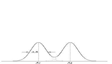
Figure 1: A bimodal probability distribution $P(A)=|f(A)|^{2}$ with peaks of width $\Delta A\equiv w$ centered at the values $A_{1}$ and $A_{2}$.

IV Examples

IV.1 Superpositions of number states

Let us start by examining a class of states for which the measure $M$ is not directly applicable (and neither is the measure proposed by Dür et al.). An example of such a state is the two-mode, bosonic state

$$(\lvert 0\rangle\otimes\lvert N\rangle+\lvert N\rangle\otimes\lvert 0\rangle)/\sqrt{2}.$$ (7)

Each of the terms in the superposition state is a two-mode number-state.

Since both components of the superposition state lack dispersion for the preferred observable they do not evolve under the preferred evolution operator $\exp[i\theta(\hat{n}_{1}-\hat{n}_{2})/2]$, where $\hat{n}_{1}$ ($\hat{n}_{2}$)is the number operator operating on the left (right) mode in the tensor product. One can ascribe this “nonevolution” to the fact that the number states are eigenstates to our preferred observable. Moreover, the number states are highly nonclassical (and consequently very fragile with respect to dissipation). Hence, although the state is in a highly excited superposition when $N$ is large, it is not in a superposition of two semiclassical states, and therefore, it is not in the spirit of Schrödinger’s example. In this case, we can still derive an interferometric macroscopality by approximating each of the superposition constituent states with a semiclassical state (cf. Fig. 2). E.g., we can compare the evolution of the superposition state with that of a coherent state having a photon number expectation value of $N$. Since the dispersion $\langle(\hat{n}-\langle\hat{n}\rangle)^{2}\rangle$ of a coherent state is $\langle\hat{n}\rangle$, we find that for such a state we get $\Delta n=\sqrt{N}$. (This result is identical to that we would have obtained if we instead had considered a two-mode coherent state.) The state in Eq. (7) becomes orthogonal for $\theta_{\text{sing}}=\pi/N$. Hence, the interferometric macroscopality of the state becomes

$$M\approx\frac{\pi/\sqrt{N}}{\pi/N}\approx\sqrt{N}.$$ (8)

Figure 2: Probability distributions for the preferred observable $n=(\hat{n}_{1}-\hat{n}_{2})/2$. The two (truncated) thick lines represent the (Kronecker-delta-like) distribution for the state $(\lvert 0\rangle\otimes\lvert N\rangle+\lvert N\rangle\otimes\lvert 0\rangle)/\sqrt{2}$ with $N=20$, which becomes orthogonal for $\theta_{\text{sing}}=\pi/N$. The dashed distributions correspond to coherent states $\lvert 0\rangle\otimes\lvert\alpha\rangle$ and $\lvert\alpha\rangle\otimes\lvert 0\rangle$ with $\lvert\alpha\rvert^{2}=\lvert\langle n\rangle\rvert=20$ and a dispersion $\Delta n\approx\sqrt{20}$, which become almost orthogonal for $\theta_{\text{sup}}\approx\pi/\sqrt{N}$. (Note that these distributions are discrete; their envelopes have been used here for simplicity.)

(See Fig. 2.) This result makes intuitive sense. In interferometry, this $\sqrt{N}$ improvement in utility denoted the difference between the standard quantum limit and the Heisenberg limit Caves (1980, 1981); Yurke et al. (1986); Grangier et al. (1987); Fabre et al. (2000); Treps et al. (2002).

The scaling would not change qualitatively if we considered a coherent state with mean photon number $N/2$, nor would it change if we had considered a slightly squeezed coherent state (with a constant squeezing parameter)

The scaling $\sqrt{N}$ for the interferometric utility is to be compared with the fragility of the state under decoherence, which scales as $N$. This means, intuitively, that the “cost” for preserving this kind of state increases faster (by a factor $\approx\sqrt{N}$) than the state’s sensitivity in interferometric application does.

This state also is a good example for the strange behavior of the disconnectivity as a measure of how macroscopic the superposition above is, for the disconnectivity is always unity for the state, irrespective of $N$. The simple explanation is that we do not increase the “size” of the state by increasing the number of modes, but instead increase only the number of excitations.

IV.2 Qubit states

A simple state that has been used as a model system to quantify the size of macroscopic superpositions is the $N$-qubit state

$$\frac{1}{\sqrt{2}}(\lvert\phi_{+}\rangle^{\otimes N}+\lvert\phi_{-}\rangle^{\otimes N}),$$ (9)

where

$$\lvert\phi_{\pm}\rangle=\cos(\varphi\pm\epsilon/2)\,\lvert 1/2\rangle+\sin(\varphi\pm\epsilon/2)\,\lvert-1/2\rangle,$$ (10)

where, without loss of generality, we have taken the two qubit basis states to be spin 1/2 eigenstates along some axis. We note that the overlap $|\langle\phi_{-}\lvert\phi_{+}\rangle|=|\cos\epsilon|$. Hence, for $0<\epsilon\ll 1$, we have $|\langle\phi_{-}\lvert\phi_{+}\rangle|^{2}\approx 1-\epsilon^{2},$ and the qubit states have a large overlap. However, as

$$|\langle\phi_{-}|^{\otimes N}\lvert\phi_{+}\rangle^{\otimes N}|=|\cos^{N}\epsilon|,$$ (11)

the many-qubit state has almost vanishing overlap as soon as $N\gg 1$ and $\epsilon>1/\sqrt{N}$. To be more specific, for $\epsilon=\arccos(e^{-1/N})\approx\sqrt{2/N}$, the overlap is $1/e$. Hence, the $N$-qubit states $\lvert\phi_{\pm}\rangle^{\otimes N}$ are almost orthogonal for $\epsilon>1/\sqrt{N}$.

In order to calculate the interferometric macroscopality of the $N$-qubit state, we choose as preferred observable the total spin $\hat{S_{r}}=\sum_{n=1}^{N}\hat{\sigma}_{n,r}$ (in units of $\hbar$) along the axis $r$ defined by the basis states. We compute the mean

$$\langle\phi_{\pm}|^{\otimes N}\hat{S_{r}}\lvert\phi_{\pm}\rangle^{\otimes N}=N\cos(2\varphi\pm\epsilon)/2,$$ (12)

and the variance

$$\langle\phi_{\pm}|^{\otimes N}\Delta\hat{S_{r}}^{2}\lvert\phi_{\pm}\rangle^{\otimes N}=N[1-\cos^{2}(2\varphi\pm\epsilon)]/4.$$ (13)

We see that in order to make the difference between the expectation values of the two superposed states $\lvert\phi_{+}\rangle^{\otimes N}$ and $\lvert\phi_{-}\rangle^{\otimes N}$ as large as possible, we should choose $\varphi=\pi/4$, i.e., the preferred observable should be along an axis forming an angle of $\pi/2$ with the superposition state’s average spin, in a Bloch-sphere representation. For this choice, $|\langle\phi_{+}|\hat{S_{r}}\lvert\phi_{+}\rangle-\langle\phi_{-}|\hat{S_{r}}\lvert\phi_{-}\rangle|=N|\sin\epsilon|\approx N\epsilon$ and the width of each spin probability distribution (the square root of each distribution’s variance) is approximately $\sqrt{N}/2$. We immediately see that as soon as $\epsilon>1/\sqrt{N}$, we get a bimodal distribution for the superposed state. This fact is supported by the condition derived previously for the two states to have a small overlap. Thus for the state (9) we get

$$M\approx\frac{N\epsilon}{\sqrt{N}/2}=2\sqrt{N}\epsilon.$$ (14)

This measure can be compared to the measure by Dür et al., where they conclude that the state’s macroscopic size is $N\epsilon^{2}$. However, their measure is based on the premise that the macroscopic size of the state $2^{-1/2}(\lvert 0\rangle^{\otimes n}+\lvert 1\rangle^{\otimes n})$ is $n$. In contrast, we find that for this state $M=n/\sqrt{n}=\sqrt{n}$. Because $\langle 0|^{\otimes n}\Delta\hat{S_{r}}^{2}\lvert 0\rangle^{\otimes n}=\langle 1|^{\otimes n}\Delta\hat{S_{r}}^{2}\lvert 1\rangle^{\otimes n}=0$, we have used the method described in the previous subsection, comparing the evolution time of the superposition state with that of a spin-coherent state with mean excitation $n$. We see that our measure is proportional to the square root of the measure of Dür et al., when a comparison is applicable. The difference between the measures can be traced to the operational questions they answer. In our case it is the state’s interference utility, in the case of Dür et al., it is how many qubits a GHZ state distilled from the macroscopic superposition contains.

Considering again Eqs. (12) and (13), we see that a choice of an observable forming a vanishing angle with the superposition state’s average spin would have led to an interference utility $M=0$: with respect to such observable, the state (9) would present very small — i.e., non-macroscopic — interference effects.

It is also worth noticing that the disconnectivity of the state (9) is $N$, irrespective of $\epsilon$, as long as $\epsilon\neq 0$. The disconnectivity vanishes only when $\epsilon=0$ exactly, even if for $\epsilon<1/\sqrt{N}$ the state does not represent a macroscopic superposition any longer. The disconnectivity’s invariance with respect to $\epsilon$ clearly demonstrates the measure’s exclusive dependence on the particle (or mode) number and its ignorance of the state of the particles (modes).

IV.3 A superposition of coherent states

Several authors have suggested to use a binary superposition of coherent states to make macroscopic superpositions. At least one experiment has been performed on such a state, that is of the form

$$\lvert\psi\rangle=\frac{1}{\sqrt{N}}(\lvert e^{i\varphi}|\alpha|\rangle+\lvert e^{-i\varphi}|\alpha|\rangle),$$ (15)

where the normalization factor

$$N=2\{1+\exp[-|\alpha|^{2}(1-\cos 2\varphi)]\cos(|\alpha|^{2}\sin 2\varphi)\}$$ (16)

and where $\hat{a}\lvert e^{i\varphi}|\alpha|\rangle=|\alpha|e^{i\varphi}\lvert e^{i\varphi}|\alpha|\rangle$. If such a state’s quadrature-amplitude distribution is measured, where the Hermitian quadrature amplitude operator is defined $\hat{a}_{2}=(\hat{a}-\hat{a}^{\dagger})/2i$, a bimodal distribution will be found, provided that the superposition “distance” $D=2|\alpha|\sin\varphi$ is sufficiently large. Hence, the preferred evolution operator is $\exp(i\theta\hat{a}_{2})$. Let us first see how a coherent state evolves towards orthogonality under this operator. The dispersion of $\hat{a}_{2}$ of the coherent state is $1/2$. Hence, we can expect the coherent state to evolve into an (almost) orthogonal after an interaction of $\theta=2\pi$.

In a more detailed calculation, we use the fact that

$$\begin{split}e^{i\theta\hat{a}_{2}}=e^{(-\theta\hat{a}^{\dagger}+\theta\hat{a})/2}&=e^{-\theta\hat{a}^{\dagger}/2}e^{\theta\hat{a}/2}e^{-[-\theta\hat{a}^{\dagger},\theta\hat{a}]/8}\\ &=e^{-\theta^{2}/8}e^{-\theta\hat{a}^{\dagger}/2}e^{\theta\hat{a}/2}.\end{split}$$ (17)

Since coherent states are eigenstates to the operator $\hat{a}$, it is easy to compute

$$\langle\alpha|e^{i\theta\hat{a}_{2}}\lvert\alpha\rangle=e^{-\theta^{2}/8}e^{i\theta\text{Im}\{\alpha\}},$$ (18)

where Im$\{z\}$ denotes the imaginary part of $z$ and where we have assumed that $|\alpha|\neq 0$. We see that the magnitude of the overlap between a coherent state and an evolved copy of itself decreases with time as $e^{-\theta^{2}/8}$. Note that the result is independent of $|\alpha|$. The evolved state never becomes fully orthogonal to the unevolved state, the overlap goes only asymptotically toward zero, but we can define $\theta_{\text{sing}}\approx 2\sqrt{2}$ as the typical “orthogonality” time. (The crude calculation above yielded $\theta_{\text{sing}}=2\pi$, roughly a factor of two higher.) In this time the (absolute value of the) overlap has decreased from unity to $1/e$. Applying the same evolution operator to the state $\lvert\psi\rangle$, above, one gets

$$\begin{split}\langle\psi|e^{i\theta\hat{a}_{2}}\lvert\psi\rangle&=\frac{2e^{-\theta^{2}/8}}{N}[\cos(\theta|\alpha|\sin\varphi)\\ &\quad+e^{-|\alpha|^{2}(1-\cos 2\varphi)}\cos(|\alpha|^{2}\sin 2\varphi)].\end{split}$$ (19)

In this case, for reasonable large values of $|\alpha|$ and $\varphi$ (when the rightmost term of the equation above is negligible) the state becomes almost orthogonal under evolution, and this first happens when

$$\theta=\theta_{\text{sup}}=\frac{\pi}{2|\alpha|\sin\varphi}.$$ (20)

Hence, the superposition’s interferometric macroscopality will be

$$M=\frac{\theta_{\text{sing}}}{\theta_{\text{sup}}}\approx\frac{2\sqrt{2}}{\pi/2|\alpha|\sin\varphi}\approx 2|\alpha|\sin\varphi.$$ (21)

Figure 3: Wigner-function representation of the coherent states $\lvert e^{i\varphi}\lvert\alpha\rvert\rangle$ and $\lvert e^{-i\varphi}\lvert\alpha\rvert\rangle$ (with $\lvert\alpha\rvert=3.1$ and $\varphi=0.5$) on the plane $\hat{a}_{1}\hat{a}_{2}$. The respective probability distributions for the preferred observable $\hat{a}_{2}$ are plotted on the left of the latter’s axis. The distance between the two distributions’ peaks is $2|\alpha|\sin\varphi$, corresponding to a $\theta_{\text{sup}}=\tfrac{\pi}{2|\alpha|\sin\varphi}$ for the superposed state to become orthogonal; the widths of the distributions is $\sim 1$, corresponding to a $\theta_{\text{sing}}\approx 2\sqrt{2}$ for each single costituent state to become orthogonal.

((See Fig. 3.) In experiments performed by Brune et al. Brune et al. (1996) on Rydberg states at microwave frequencies, a $|\alpha|$ of 3.1 was achieved, and $\varphi$ was varied between approximately $0.1-0.5$ rad. Hence, an interferometric macroscopality of $\approx 6.2\sin 0.5\approx 3$ was achieved. However, at the largest angles $\varphi$ measured, the state had already decohered substantially, so the superposition state was no longer a pure superposition. It is worth noticing that the decoherence, manifested in the decrease of the Ramsey interference fringes measured in the experiment, scales as $\exp(-D^{2}/2)$. The decoherence time is hence proportional to the interferometric macroscopality squared of the state. This is the same result we found for a rather different state in Sec. IV.2. The result suggest that that the found relation between the decoherence and the interferometric macroscopality of the state is quite general. The result also indicates that it will be difficult to reap the full utility of macroscopic superposition states in applications, unless dissipation is kept to a minimum.

IV.4 Molecule interferometry

A series of experiments have been performed on diffraction of molecules with increasing atomic weight. The effort started in the 1930’s with interference experiments with H₂ (weight 2 in atomic mass units), but recently the field has used increasingly larger molecules going from He₂, Li₂, Na₂, K₂ and I₂ (with weights 8, 14, 46, 78, and 254 atomic mass units, respectively) to substantially heavier molecules such as C₆₀, C₇₀ to C₆₀F₄₈ (with weights 720, 840 and 1632 atomic mass units, respectively). In one of the recent experiments of this type Arndt et al. (1999), a collimated beam of C₆₀ molecules was diffracted by a free-standing SiN_x grating consisting of 50 nm wide slits with a 100 nm period $D$. A tree-peaked diffraction pattern was observed a distance $L=1.25$ m behind the grating by means of a scanning photo-ionization stage followed by a ion detection unit. The distance from the central peak and the nodes on each side of it was about 12 $\mu$m.

To analyze the experiment in terms of macroscopic superpositions, we note that the molecular beam intensity is such that the molecules are diffracting one by one. Hence, we need not invoke quantum mechanics to explain the diffraction pattern, but we can simply model the experiment in terms of first-order wave interference. We note that for a single slit of width $d$, the molecule intensity in the direction $\theta$ from the slit normal direction is proportional to

$$I\propto\int_{-d/2}^{d/2}e^{ikx\sin(\theta)}\approx\int_{-d/2}^{d/2}e^{ikx\theta},$$ (22)

where $x$ is the position coordinate across the slit, $k$ is the molecule’s de Broglie wave vector, we have assumed a constant molecular beam amplitude across the slit, and diffraction close to the normal has been considered. We see that in a slit diffraction experiment, the position $x$ is the preferred observable and the parameter $\theta$ can be interpreted as the diffraction angle. We can express $k$ in the molecular beam velocity $v=220$ ms^-1, and the molecular weight $m=720$ atomic mass units as $k=2\pi mv/h$, where $h$ is Planck’s constant. We find that orthogonality occurs when $\theta=\theta_{\text{sing}}=h/dmv$. Experimentally, this means that the single slit diffraction pattern has its first node at this angle, or at a distance $\approx hL/dmv$ from the diffraction peak center in the observation plane. In a thought single slit experiment with the same experimental parameter as in the experiment referred to above, the node should have been found by the ionization detector about 63 $\mu$m from the diffraction pattern center. In the real experiment, the first node (indicating orthogonality) was found 12 $\mu$m from the central diffraction peak. Since $\theta_{\text{sup}}$ scales proportionally to this distance, we can compute the interferometric macroscopality of the superposition state as $M=63/12\approx 5.2$. This is perhaps smaller than one would expect.

In a later refinement Nairz et al. (2003), the molecular beam was velocity filtered around 110 ms^-1. In this case the the coherence length of the molecules increased significantly, resulting in several diffraction fringes. However, the interferometric macroscopality of the state was equal to that in the earlier experiment. With a single slit, the first diffraction node would have been expected at 125 $\mu$m from the diffraction center. With the grating the first node is found at 24 $\mu$m from the center. Thus, $M=125/24\approx 5.2$.

From the considerations above, we see that the path towards larger interferometric macroscopality lies not in employing molecules with larger mass, but only in making the relative slit separation greater.

It is of course an impressive fact to produce a matter wave consisting of relatively heavy molecules with a ${}>100\mathrm{nm}$ transverse coherence length. However, a matter wave is not automatically the same as a macroscopic superposition state in the sense of Schrödinger.

IV.5 SQUID interference

Another physical system where macroscopic superposition states have been created and measured, is superconducting interference devices (SQUIDs). These devices consist of a superconducting wire loop incorporating Josephson junctions Friedman et al. (2000); van der Wal et al. (2000). In these junctions, the magnetic flux through the ring is quantized in units of the flux quantum $\phi_{0}=h/2e$, where $e$ is the unit charge. The supercurrent in the loop can be controlled by applying an external magnetic field. When the external field magnetic flux $\phi_{x}$ through the ring is about one half a flux quanta, the supercurrent in the ring can either flow in such a way that the induced magnetic flux cancels $\phi_{x}$ or so that it augments it. The corresponding “fluxoid” states correspond to zero and one flux quanta respectively. The SQUID potential $U$ is given of the sum between the magnetic energy of the ring and the Josephson coupling energy of the junction(s):

$$U=\frac{1}{2}\left[\frac{\phi_{0}^{2}}{L}\left(\frac{\phi-\phi_{x}}{\phi_{0}}\right)^{2}-\frac{\phi_{0}I_{c}}{\pi}\cos(2\pi\phi/\phi_{0})\right],$$ (23)

where $L$ is the the ring inductance and $I_{c}$ is the junction critical current. By tuning the induced flux, a double-well potential as a function of the flux $\phi$ that threads the ring can be created. To a first approximation, each well can be approximated by a harmonic potential with (approximately) equidistantly spaced energy states. However, there is a finite barrier between the wells, and this barrier can be tuned with the help of the applied magnetic field. For certain values of the external field, an excited level of each of the wells line up, and tunnelling between the states is possible. In one of the experiments Friedman et al. (2000), the tunnelling transition probability is monitored as a function of the applied magnetic flux and the frequency of a microwave frequency pulse. Under certain conditions it is possible to create an equal superposition of the fluxoid states $\lvert 0\rangle$ and $\lvert 1\rangle$. The odd and even superposition states differ in energy by about 0.86 $\mu$eV ($\Delta E/k_{B}\approx 0.1$ K, where $k_{B}$ is Boltzmann’s constant).

To analyze the fluxoid superposition state, the preferred operator is the magnetic flux through the ring. The difference in the (mean) magnetic flux of the two bare fluxoid states $\lvert 0\rangle$ and $\lvert 1\rangle$ is deduced to be about $\phi_{0}/4$. In order to estimate the interferometric macroscopality of this state we need to estimate the flux interaction needed to evolve a “classical” flux state into an orthogonal one. Since the considered fluxoid states are discrete, they nominally do not evolve under the action of the flux operator (only their overall phase evolves). To make an estimate of how rapid the evolution of a “classical” flux state would be, we use the fact that the SQUID’s potential wells are approximately harmonic, and that classically, the state would be confined to only one of the wells. We can then construct a coherent flux state confined to one of the wells.

To estimate the state’s dispersion (width) when expressed in the flux operator, we note that the potential well level spacing of the SQUID $\Delta{\cal E}$ in each potential well is about is about 86 $\mu$eV ($\Delta{\cal E}/k_{B}\approx 1$ K). The numerical values for the potential are $\phi_{0}^{2}/2L\approx 55.6$ meV ($\phi_{0}^{2}/2Lk_{B}\approx 645$ K), and $\phi_{0}I_{c}/2\pi\approx 6.5$ meV ($\phi_{0}I_{c}/2\pi k_{B}\approx 76$ K). In a (mechanical) harmonic oscillator, we have $U=\kappa x^{2}/2$, an energy level spacing of $\hbar\omega=\hbar\sqrt{\kappa/m}$, and a position dispersion of

$$\Delta x\approx\frac{1}{2}\sqrt{\frac{\hbar}{\omega m}}=\frac{1}{2}\sqrt{\frac{\hbar}{\sqrt{\kappa m}}},$$ (24)

where $\kappa$ is the spring constant and $m$ is the oscillator mass. Taylor expanding the potential in (23) around the point $\phi_{x}=0$ and using the analogy with the mechanical harmonic oscillator, we find that the flux dispersion of the flux coherent state is

$$\Delta\phi\approx\frac{\phi_{0}}{2}\sqrt{\frac{1}{1290+4\pi^{2}76}}\approx 7.6\cdot 10^{-3}\phi_{0}.$$ (25)

Hence, the state’s interferometric macroscopality is

$$M=\frac{\phi_{0}/4}{7.6\cdot 10^{-3}\phi_{0}}\approx 33.$$ (26)

This interferometric macroscopality is impressive, but significantly different from what one might naively guess, considering that the flux difference between the states $\lvert 0\rangle$ and $\lvert 1\rangle$ corresponds to a local magnetic moment of about $10^{10}$ $\mu_{B}$ Friedman et al. (2000).

IV.6 Quantum superpositions of a mirror

In the literature it has been proposed that emerging technology will soon allow one to put a mirror into a superposition of positions Marshall et al. (2002). The idea is to suspend a small ($10\times 10\times 10$ $\mu$m) mirror at the tip of a high Q-value cantilever. The mirror would form the end-mirror of a plano-concave, high-Q cavity. This cavity would form one arm of a Michelson interferometer. In the other arm there would be a rigid cavity with equal resonance frequency and finesse. When a single photon is incident on the Michelson interferometer input port, with probability $1/2$, the photon would either be found in the rigid cavity or in the cavity with the cantilever suspended mirror. The photon pressure would shift the position of the suspended mirror, and relatively quickly, the position of the cantilever and the photon state would be entangled. The authors proceed to analyze how well this entanglement could be detected by detecting in what port the photon exits the Michelson interferometer as a function of time. Quite intuitively, if the photon exerts pressure on the mirror for a whole oscillation period of the mirror, the work exerted by the photon on the mirror when the two are moving codirectionally, is cancelled by the work the mirror exerts on the photon mode when he mirror and photon move contradirectionally. Hence, there will be a revival in the photon interference visibility after an interaction time equal to the mirror oscillation period.

Of course, dissipation (decoherence) will impede one to observe this revival, but the authors deduce that in a cool enough environment, it is possible to find somewhat realistic parameters allowing the quantum superposition to be detected through the photon’s visibility revival. The authors suggest that under these conditions, the separation between the two mirror positions in the superposition correspond to the width (dispersion) of a coherent state wavepacket. This immediately lets us deduce that the interferometric macroscopality of the suggested experiment is of the order unity, in spite of involving an astronomic number of atoms, $\sim 10^{14}$.

V Conclusions

In this paper, a measure has been presented to quantify how “macroscopic” some superpositions realized in different experiments are. The measure is based on the utility of the superposition state as a probe in interference experiments, quantified by the difference in time or, more generally, in interaction strength needed to make a macroscopic superposition or, respectively, the single macroscopic states evolve into orthogonal states by means of a unitary transformation generated by a particular preferred observable.

The proposed measure gives values for the “interferometric macroscopalities” of recent experiments that are perhaps smaller than expected; this is due to the fact that the measure is not directly related to the number of particles, or excitations, involved in the experiment, but rather to the interference properties deriving from large separations of two superposed states as measured by the preferred observable.

Let us finally remark again that the issue about the word ‘macroscopic’ is very subjective, but it is interesting as well, and can provide some insight in the way we look and use quantum and non-quantum mechanical concepts.