Combinatorial Physics, Normal Order and Model Feynman Graphs

Allan I. \surnameSolomon†§ Université Pierre et Marie Curie
Laboratoire de Physique Théorique des Liquides, CNRS UMR 7600
Tour 16, $5^{i\grave{e}me}$ étage, 4, place Jussieu, F 75252 Paris, Cedex 05, France
e-mail: penson@lptl.jussieu.fr
H. Niewodniczański Institute of Nuclear Physics, Polish Academy of Sciences
Department of Theoretical Physics
ul. Radzikowskiego 152, PL 31-342 Kraków, Poland
e-mail: pawel.blasiak@ifj.edu.pl, andrzej.horzela@ifj.edu.pl
§The Open University
Physics and Astronomy Department
Milton Keynes MK7 6AA
e-mail: a.i.solomon@open.ac.uk
§§LIFAR, Université de Rouen
76821 Mont-Saint Aignan Cedex, France
e-mail: gduchamp2@free.fr
   Pawel \surnameBlasiak†‡ Université Pierre et Marie Curie
Laboratoire de Physique Théorique des Liquides, CNRS UMR 7600
Tour 16, $5^{i\grave{e}me}$ étage, 4, place Jussieu, F 75252 Paris, Cedex 05, France
e-mail: penson@lptl.jussieu.fr
H. Niewodniczański Institute of Nuclear Physics, Polish Academy of Sciences
Department of Theoretical Physics
ul. Radzikowskiego 152, PL 31-342 Kraków, Poland
e-mail: pawel.blasiak@ifj.edu.pl, andrzej.horzela@ifj.edu.pl
§The Open University
Physics and Astronomy Department
Milton Keynes MK7 6AA
e-mail: a.i.solomon@open.ac.uk
§§LIFAR, Université de Rouen
76821 Mont-Saint Aignan Cedex, France
e-mail: gduchamp2@free.fr
   Gerard \surnameDuchamp§§ Université Pierre et Marie Curie
Laboratoire de Physique Théorique des Liquides, CNRS UMR 7600
Tour 16, $5^{i\grave{e}me}$ étage, 4, place Jussieu, F 75252 Paris, Cedex 05, France
e-mail: penson@lptl.jussieu.fr
H. Niewodniczański Institute of Nuclear Physics, Polish Academy of Sciences
Department of Theoretical Physics
ul. Radzikowskiego 152, PL 31-342 Kraków, Poland
e-mail: pawel.blasiak@ifj.edu.pl, andrzej.horzela@ifj.edu.pl
§The Open University
Physics and Astronomy Department
Milton Keynes MK7 6AA
e-mail: a.i.solomon@open.ac.uk
§§LIFAR, Université de Rouen
76821 Mont-Saint Aignan Cedex, France
e-mail: gduchamp2@free.fr
   Andrzej \surnameHorzela Université Pierre et Marie Curie
Laboratoire de Physique Théorique des Liquides, CNRS UMR 7600
Tour 16, $5^{i\grave{e}me}$ étage, 4, place Jussieu, F 75252 Paris, Cedex 05, France
e-mail: penson@lptl.jussieu.fr
H. Niewodniczański Institute of Nuclear Physics, Polish Academy of Sciences
Department of Theoretical Physics
ul. Radzikowskiego 152, PL 31-342 Kraków, Poland
e-mail: pawel.blasiak@ifj.edu.pl, andrzej.horzela@ifj.edu.pl
§The Open University
Physics and Astronomy Department
Milton Keynes MK7 6AA
e-mail: a.i.solomon@open.ac.uk
§§LIFAR, Université de Rouen
76821 Mont-Saint Aignan Cedex, France
e-mail: gduchamp2@free.fr
   Karol A. \surnamePenson Université Pierre et Marie Curie
Laboratoire de Physique Théorique des Liquides, CNRS UMR 7600
Tour 16, $5^{i\grave{e}me}$ étage, 4, place Jussieu, F 75252 Paris, Cedex 05, France
e-mail: penson@lptl.jussieu.fr
H. Niewodniczański Institute of Nuclear Physics, Polish Academy of Sciences
Department of Theoretical Physics
ul. Radzikowskiego 152, PL 31-342 Kraków, Poland
e-mail: pawel.blasiak@ifj.edu.pl, andrzej.horzela@ifj.edu.pl
§The Open University
Physics and Astronomy Department
Milton Keynes MK7 6AA
e-mail: a.i.solomon@open.ac.uk
§§LIFAR, Université de Rouen
76821 Mont-Saint Aignan Cedex, France
e-mail: gduchamp2@free.fr
Abstract

The general normal ordering problem for boson strings is a combinatorial problem. In this talk we restrict ourselves to single-mode boson monomials. This problem leads to elegant generalisations of well-known combinatorial numbers, such as Bell and Stirling numbers. We explicitly give the generating functions for some classes of these numbers. Finally we show that a graphical representation of these combinatorial numbers leads to sets of model field theories, for which the graphs may be interpreted as Feynman diagrams corresponding to the bosons of the theory. The generating functions are the generators of the classes of Feynman diagrams.

keywords:
combinatorics, normal order, Feynman diagrams.
{opening}

1 Boson Normal Ordering

In this note we give a brief review of the combinatorial properties associated with the normal ordering of bosons, and the model Feynman graphs which result.

Combinatorial sequences appear naturally in the solution of the boson normal ordering problem [1], [2].

The normal ordering problem for canonical bosons $[a,a^{\dagger}]=1$ is related to certain combinatorial numbers $S(n,k)$ called Stirling numbers of the second kind through [3]

$\displaystyle(a^{\dagger}a)^{n}=\sum_{k=1}^{n}S(n,k)(a^{\dagger})^{k}a^{k},$ (1)

with corresponding numbers $B(n)=\sum_{k=1}^{n}S(n,k)$ called Bell numbers. In fact, for physicists, these equations may be taken as the definitions of the Stirling and Bell numbers. For quons (q-bosons) satisfying $[a,a^{\dagger}]_{q}\equiv aa^{\dagger}-qa^{\dagger}a=1$ a natural q-generalisation [4] of these numbers is

$\displaystyle(a^{\dagger}a)^{n}=\sum_{k=1}^{n}S_{q}(n,k)(a^{\dagger})^{k}a^{k}.$ (2)

In the canonical boson case, for integers $n,r,s>0$ we define generalized Stirling numbers of the second kind $S_{r,s}(n,k)$ through ($r\geq s$):

$\displaystyle[(a^{\dagger})^{r}a^{s}]^{n}=(a^{\dagger})^{n(r-s)}\sum_{k=s}^{ns}S_{r,s}(n,k)(a^{\dagger})^{k}a^{k},$ (3)

as well as generalized Bell numbers $B_{r,s}(n)$

$\displaystyle B_{r,s}(n)=\sum_{k=s}^{ns}S_{r,s}(n,k).$ (4)

For both $S_{r,s}(n,k)$ and $B_{r,s}(n)$ exact and explicit formulas have been found [1, 2]. We refer the interested reader to these sources for further information on those extensions. However, in this note we shall only deal with the classical Bell and Stirling numbers, corresponding to $B_{1,1}(n)$ and $S_{1,1}(n)$ in our notation.

2 Generating Functions

In general, for combinatorial numbers $g(n)$ we may define an exponential generating function $G(x)$ through [6]

$$G(x)=\sum_{n=0}^{\infty}g(n)\frac{x^{n}}{n!}.$$ (5)

For the Bell numbers, the generating function takes the particularly nice form[5]

$$G(x)=\sum_{n=0}^{\infty}B(n)\frac{x^{n}}{n!}=\exp(\exp(x)-1).$$ (6)

Some initial terms of the sequence $\{B(n)\}$ are $\{1,2,5,15,52,203,877,\ldots\}$.

3 Graphs

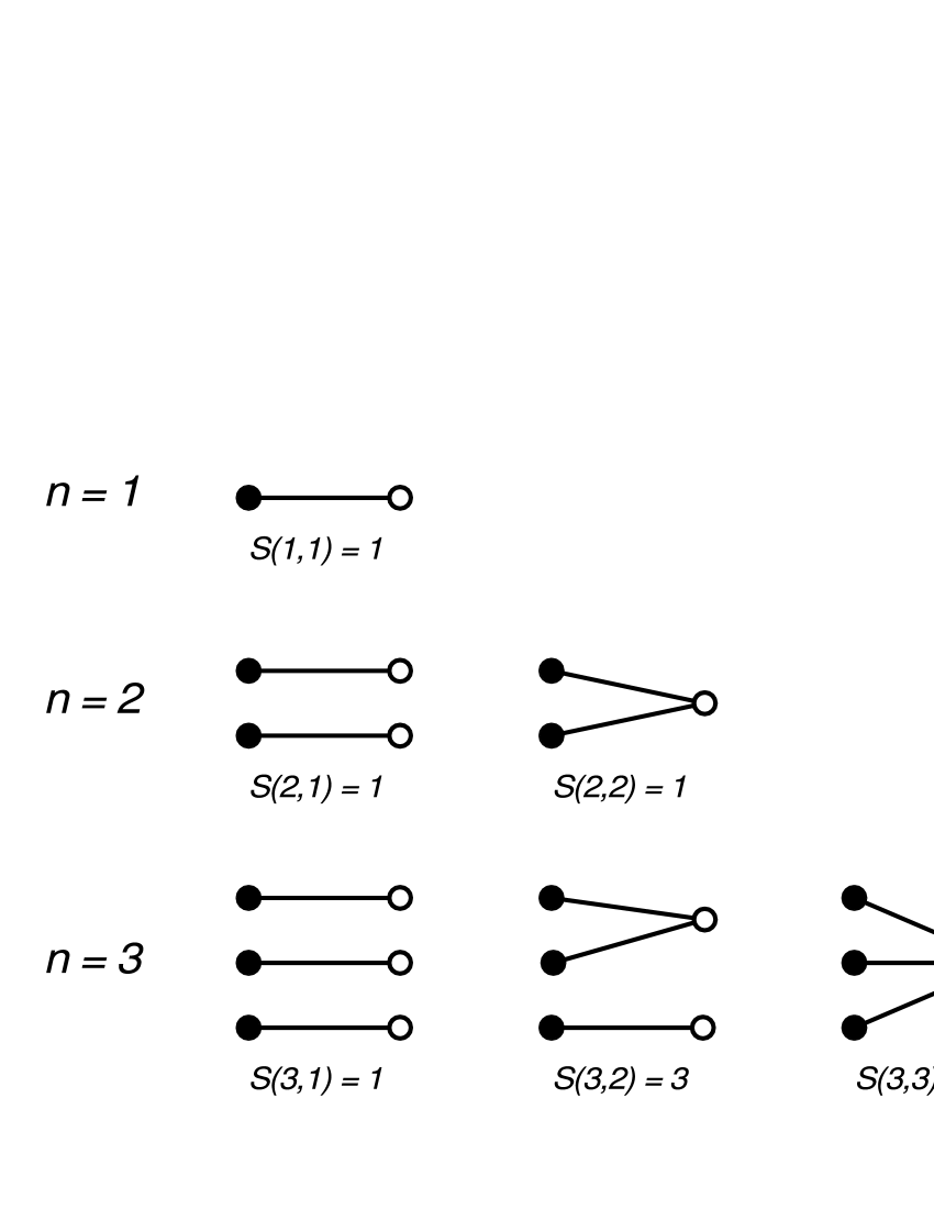
A convenient way of representing combinatorial numbers is by means of graphs. To illustrate this, we now consider a graphical method for illustrating the combinatorial numbers associated with the normal order expansion of $(a^{\dagger}a)^{n}$.

Refer to caption
Figure 1: Arrow graphs for $(a^{\dagger}a)^{n}\;\;\;n=1,2,3.$

A single arrow represents a “time-segment” of a line corresponding to the “propagator” $(a^{\dagger}a)$. Thus we may concatenate one, two or more arrows to form a single line, or propagator $(a^{\dagger}a)$. However, two lines correspond to two distinct propagators ${a^{\dagger}}^{2}a^{2}$, and so on. Further, the constitutent arrows are labelled, for example by time, and so they may only be concatenated respecting the time ordering. These rules are illustrated by the diagrams of Figure 1, in which we consider the cases of 1, 2, and 3 arrows respectively. We have pre-emptively labelled these numbers as Bell numbers - which fact we demonstrate below. For the case of 4 arrows (Figure 2) we have additionally given the individual associated symmetry factors (in fact Stirling numbers) which add to $B(4)=15$. It should be clear from this illustration how the time-ordering rules are applied to give the symmetry coefficients. Thus there is only one way in which we can concatenate 4 arrows respecting time-ordering (first grouping), 4 ways in which we can divide the arrows into a set of 3 and 1, and so on.

Refer to caption
Figure 2: Arrow graphs for $(a^{\dagger}a)^{4}.$

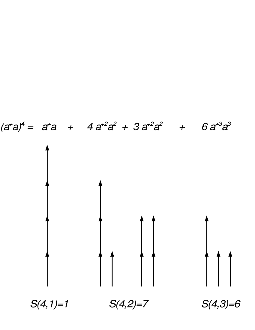
From these first few examples it would seem that these graphs are essentially like the Feynman Diagrams of a zero-dimensional (no integration) Model Field Theory associated with $H=a^{\dagger}a$. In other words, at order $n$ the total number of graphs would appear to be $B(n)$ while the individual coefficients of ${a^{\dagger}}^{k}a^{k}$ are given by $S(n,k)$. In order to show that this is indeed the case, we must be able to count the number of graphs associated with a given number $n$ of arrows. To do this we can use the First of Three Great Results.

4 First Great Result

This First Great Result is sometimes known as the connected graph theorem [7]. It states that if $C(x)=\sum_{n=1}^{\infty}c(n)x^{n}/n!$ is the generating function of labelled connected graphs, viz. $c(n)$ counts the number of connected graphs of order $n$, then

$$A(x)=\exp(C(x))$$ (7)

is the generating function for all graphs.

We may apply this very simply to the case of the arrow graphs above. For each order $n$, the connected graphs consist of the single graph obtained by concatenating all the arrows into one propagator. Therefore for each $n$ we have $c(n)=1$; whence, $C(x)=exp(x)-1.$ It follows that the generating function for all the arrow graphs $A(x)$ is given by

$$A(x)=\exp(\exp(x)-1)$$ (8)

which is the generating function for the Bell numbers.

Such graphs may be generalised to give graphical representations for the extensions $B_{r,s}(n)$ [8].

However, just as an abstract group is capable of more than one presentation, there are many graphical representations for a given combinatorial sequence; and we now give an alternative one for the numbers $B(n),S(n,k)$ due to Bender and collaborators [9], [10].

5 Second Great Result

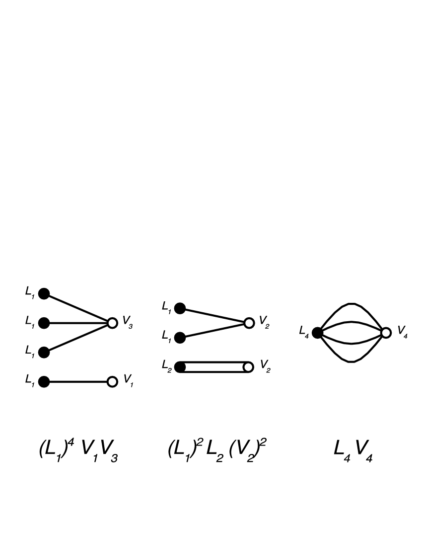
As before, we shall be counting lines. A line starts from a white dot, the origin, and ends at a black dot, the vertex. What we refer to as origin and vertex is, of course, arbitrary. At this point there are no other rules, although we are at liberty to impose further restrictions; a white dot may be the origin of 1,2,3,… lines, and a black dot the vertex for 1,2,3,… lines. We may further associate strengths $V_{s}$ with each vertex receiving $s$ lines, and multipliers $L_{m}$ with a white dot which is the origin of $m$ lines. Again $\{V_{s}\}$ and $\{L_{m}\}$ play symmetric roles; in this note we shall only consider cases where the $L_{m}$ are either 00 or $1$.

We illustrate these rules for four different graphs corresponding to $n=4$.

Refer to caption
Figure 3: Some examples of 4-line graphs.

There is an generating function $G(x,V,L)$ which counts the number $g(n)$ of graphs with $n$ lines arising from the above rules [11]:

$\displaystyle G(x,V,L)$ $\displaystyle=$ $\displaystyle\left.\exp(\sum_{m=1}^{\infty}L_{m}\frac{x^{m}}{m!}\frac{d^{m}}{dy^{m}})\exp(\sum_{s=1}^{\infty}V_{s}\frac{y^{s}}{s!})\right|_{y=0}$ (9)
$\displaystyle\equiv$ $\displaystyle\sum_{n=0}^{\infty}g(n)\frac{x^{n}}{n!}$

Consider the following example: $L_{m}=0$ for all $m\neq 1$, that is, we allow only one line from each origin (with multiplier 1); there is no restriction on the number of lines to a vertex, and $V_{s}=1$ for all $s$. We give an example of the cases $n=1,2,3,4$ in Figure 4. Note that for correct counting the lines should be labelled, as they were in the case of the arrows above.

The generating function $G(x)$ which counts the lines corresponding to the above rules follows immediately from Eq.(9)

$\displaystyle G(x)$ $\displaystyle=$ $\displaystyle\left.\exp(\sum_{m=1}^{\infty}L_{m}\frac{x^{m}}{m!}\frac{d^{m}}{dy^{m}})\exp(\sum_{s=1}^{\infty}V_{s}\frac{y^{s}}{s!})\right|_{y=0}$ (10)
$\displaystyle=$ $\displaystyle\left.\exp(\frac{x}{1!}\frac{d}{dy})\exp(\sum_{s=1}^{\infty}\frac{y^{s}}{s!})\right|_{y=0}$
$\displaystyle=$ $\displaystyle\left.\exp(xd/dy)\exp(e^{y}-1)\right|_{y=0}$
$\displaystyle=$ $\displaystyle\exp(e^{x}-1)\equiv\sum_{n=0}^{\infty}{B(n)\frac{x^{n}}{n!}}.$

The penultimate step is a consequence of the Taylor expansion.

We thus have yet another representation of the integer sequence $\{B(n)\}$. Note that when $L\equiv\{L_{m}\}$ and $V\equiv\{V_{s}\}$ are integer sequences we obtain an integer sequence from Eq.(9). A convenient method of obtaining the resulting integer sequence is afforded by the next useful result.

Refer to caption
Figure 4: Graphs of second type for $B(n),\;\;\;n=1,2,3.$

6 Third Great Result

Straightforward manipulation of series shows the following: Define

$$A_{i}(x)=\sum_{n=0}^{\infty}a_{i}(n)\frac{x^{n}}{n!}\;\;\;\;\;i=1,2,3.$$ (11)

Then if

$$\left.A_{1}(xd/dy)A_{2}(y)\right|_{y=0}=A_{3}(x)$$ (12)

we have

$$a_{3}(n)=a_{1}(n)a_{2}(n).$$ (13)

This is a useful and rather surprising equality.

Using the results of the previous section, Eq.(13) enables us to create graphical representations of products of integral sequences. For example: if in the case above we chose $L_{m}=1$ for all $m$, enabling any number of lines from each origin (with multiplier 1), the resulting sequence of graphs would have given us a representation of the integer sequence $\{B(n)^{2}\}$ [9].

We exemplify the possibilities offered by application of the Third Great Result by our two final examples.

Example 1: Generating function for the sequence $\{B(n)B(n+1)\}$.

From Eqs.(11) and (13), the required generating function is given by

$$G(x,V,L)=\left.A_{1}(xd/dy)A_{2}(y)\right|_{y=0}$$ (14)

where $A_{1}(x)$ is the generating function for $\{B(n)\}$ and $A_{2}(x)$ is that of $\{B(n+1)\}$. Note that $A_{1}(x)=\exp(\exp(x)-1)$ from Eq.(8), while $A_{2}(x)=(d/dx)A_{1}(x)=\exp(\exp(x)-1+x)$.

This shows that the graphs for the sequence $\{B(n)B(n+1)\}$ may be obtained by putting $L_{m}=1$ for all $m$, so that there are any number of lines emanating from an origin, and with multiplicity 1. For the sequence $\{B(n+1)\}$ we have $V_{s}=1$ for all $s\neq 2$ and $V_{2}=2$, so that any number of lines may end at a vertex, and all have strength 1 except for the case where two lines meet at a vertex, when the strength is 2. The generating function is, according to Eq.(13),

$$G_{1}(x,V,L)=\sum_{n=0}^{\infty}B(n)B(n+1)\frac{x^{n}}{n!}.$$ (15)

It may be explicitly obtained after some formal algebraic manipulation based on the Dobiński formula [12]

$$B(n)=\frac{1}{e}\sum_{k=0}^{\infty}\frac{k^{n}}{k!}$$ (16)

as

$$G_{1}(x,V,L)=\sum_{k=0}^{\infty}\frac{1}{k!}\exp(\exp((k+1)x)-2).$$ (17)

The formal series (17) diverges for all $x>0$, although having finite Taylor coefficients for $x=0$. Such formal series are nevertheless useful in representing integer sequences.

Example 2: In our last example we retain all the derivative terms in Eq.(11) but choose $V_{1}=V_{2}=1;V_{s}=0,s>2$, thus allowing vertices where at most two lines meet. The corresponding generating function is defined by

$$G_{2}(x,V,L)=\sum_{n=0}^{\infty}B(n)I(n)\frac{x^{n}}{n!}$$ (18)

where the Involution numbers $I(n)=1,2,4,10,26,76,\ldots$ are defined through their generating function

$$G_{I}(x)=\exp(x+\frac{x^{2}}{2})=\sum_{n=0}^{\infty}I(n)\frac{x^{n}}{n!}$$ (19)

and are special values of the Hermite polynomials $H_{n}(x)$

$$I(n)=H_{n}(\frac{1}{\sqrt{2}i})/(-\sqrt{2}i)^{n}.$$

Consequently

$\displaystyle G_{2}(x,V,L)$ $\displaystyle=$ $\displaystyle\sum_{n=0}^{\infty}B(n)H_{n}(\frac{1}{\sqrt{2}i})(\frac{-x}{\sqrt{2}i})^{n}/n!$ (20)
$\displaystyle=$ $\displaystyle\sum_{k=0}^{\infty}\frac{1}{k!}\exp(kx(1+\frac{kx}{2})-1).$ (21)

In obtaining Eq.(21) we have used the standard form of the generating function of the Hermite polynomials. Again, we must consider the series Eqs.(20) and (21) as formal power series, since for example they diverge for $x>0$.

In conclusion, we emphasize that the expressions of Eqs.(17) and (21) constitute exact solutions of Model Field Theories defined by the appropriate sets $\{V_{s}\}$ and $\{L_{m}\}$. Many other applications and extensions of the ideas sketched in this note will be found in [8].

Acknowledgements.
We thank Carl Bender and Itzhak Bars for interesting discussions.

References

  • [1] Blasiak, P., Penson, K.A. and Solomon, A.I.: The general boson normal ordering problem, Phys. Lett. A 309 (2003), 198.
  • [2] Blasiak, P., Penson, K.A. and Solomon, A.I.: The boson normal ordering problem and generalized Bell numbers, Ann. Comb. 7 (2003), 127.
  • [3] Katriel, J.: Combinatorial aspects of boson algebra, Lett. Nuovo Cimento 10 (1974), 565.
  • [4] Katriel, J.: Bell numbers and coherent states, Phys. Lett. A. 273 (2000), 159.
  • [5] Comtet, L.: Advanced Combinatorics, Reidel, Dordrecht, 1974.
  • [6] Wilf, H.S.: Generatingfunctionology, Academic Press, New York, 1994.
  • [7] Stanley, R.P: Enumerative Combinatorics vol.2, Cambridge University Press, 1999; Riddel, R.J. and Uhlenbeck, G.E.: On the theory of the virial development of the equation of state of monoatomic gases, J. Chem. Phys. 21 (1953) 2056; Aldrovandi, R.: Special Matrices of Mathematical Physics, World Scientific, Singapore, 2001.
  • [8] Blasiak, P., Duchamp, G., Horzela, A., Penson, K.A. and Solomon, A.I.: Model combinatorial field theories, to be published.
  • [9] Bender, C.M, Brody, D.C. and Meister, B.K.: Quantum field theory of partitions, J.Math. Phys. 40 (1999) 3239; Bender, C.M., Brody, D.C., and Meister, B.K.: Combinatorics and field theory, Twistor Newsletter 45 (2000) 36.
  • [10] Bender, C.M. and Caswell, W.E.: Asymptotic graph counting techniques in $\psi^{2N}$ field theory, J. Math. Phys 19 (1978) 2579; Bender, C.M., Cooper, F., Guralnik, G.S., Sharp, D.H., Roskies, R. and Silverstein, M.L.: Multilegged propagators in strong-coupling expansions, Phys. Rev. D 20 (1979) 1374.
  • [11] Vasiliev, N.A.: Functional Methods in Quantum Field Theory and Statistical Physics, Gordon and Breach Publishers, Amsterdam, 1998.
  • [12] Blasiak, P., Penson, K.A. and Solomon, A.I.: Dobiński-type relations and the log-normal distribution, J. Phys. A: Math. Gen. 36 (2003), L273.