Quantum Random Walk on the Line as a Markovian Process

Abstract

We analyze in detail the discrete–time quantum walk on the line by separating the quantum evolution equation into Markovian and interference terms. As a result of this separation, it is possible to show analytically that the quadratic increase in the variance of the quantum walker’s position with time is a direct consequence of the coherence of the quantum evolution. If the evolution is decoherent, as in the classical case, the variance is shown to increase linearly with time, as expected. Furthermore we show that this system has an evolution operator analogous to that of a resonant quantum kicked rotor. As this rotator may be described through a quantum computational algorithm, one may employ this algorithm to describe the time evolution of the quantum walker.

1 Introduction

The study of computational devices based upon quantum mechanics, i.e. Quantum Computation, has drawn the attention of researchers in the last few decades [1, 2]. The recent advances in technology that allow to construct and preserve almost perfectly quantum states, have opened the possibility of building useful quantum computing devices. However, relatively few quantum algorithms that outperform classical ones have been found [3, 4]. The classical random walk is an example of stochastic motion that has found classical applications in many fields. The quantum version of this problem has several features which are markedly different from the classical walk [5, 6]. As some classical algorithms are based on random walks, it seems natural to ask whether quantum random walks might be a useful tool for quantum computation [7].

The discrete–time quantum walk on the line was introduced as a generalization of the classical random walk to the quantum world. Here, we will focus on the discrete–time quantum random walk on the line from a new perspective which emphasizes the role of coherence as the physical reason behind the striking differences found in the quantum version of the walk. We first briefly introduce the basic notions and notation relative to the discrete–time quantum walk on the line. Consider a particle that can move freely over a series of interconnected sites. The discrete quantum walk on the line is implemented by introducing an additional degree of freedom, the chirality, which can take two values: “left” or “right”, $|L\rangle$ or $|R\rangle$, respectively. This is the quantum analog of the classical decision of the random walker. At every time step, a rotation (or, more generally, a unitary transformation) of the chirality takes place and the particle moves according to its final chirality state. The global Hilbert space of the system is the tensor product $H_{s}\otimes H_{c}$ where the Hilbert space associated to the motion on the line is $H_{s}$ and the chirality Hilbert space is $H_{c}$.

If one is only interested in the properties of the probability distribution, it has been claimed [5, 8, 9] that it suffices to consider unitary transformations which can be expressed in terms of a single real angular parameter $\theta$. Let us call the operators that translate the walker one site to the left (right) on the line in $H_{s}$ as $T_{-}$ ($T_{+}$), and $|L\rangle\langle L|$ and $|R\rangle\langle R|$ the chirality projector operators in $H_{c}$. We consider transformations of the form,

$$U(\theta)=\left\{T_{-}\otimes|L\rangle\langle L|+T_{+}\otimes|R\rangle\langle R|\right\}\circ\left\{I\otimes K(\theta)\right\},$$ (1)

where $K(\theta)=\sigma_{z}e^{i\theta\sigma_{y}}$, $I$ is the identity operator in $H_{s}$, and $\sigma_{y}$ and $\sigma_{z}$ are Pauli matrices acting in $H_{c}$. The unitary operator $U(\theta)$ evolves the state by one time step,

$$|\Psi(t+1)\rangle=U(\theta)|\Psi(t)\rangle.$$ (2)

One of the most remarkable characteristics of the quantum walk on the line is that it spreads over the line faster than its classical counterpart. In this work, we apply a general approach which leads to an physical insight of why this is so. To do this, we rewrite the evolution equation as the sum of two separate terms, one responsible for the classical–like diffusion and the other for the quantum coherence [10]. As we shall see, the terms responsible for the diffusion obey a master equation, as is typical of Markovian processes, while the other includes the interference terms needed to preserve the unitary character of the quantum evolution. In Section 2, we review the decomposition of the evolution in these two terms. In Section 3, we obtain analytical expressions for the first and second moments of the probability distribution for these terms, in the case of the quantum random walker. Finally, in Section 4, we discuss our conclusions.

2 Derivation of the Master Equation from the unitary evolution

In a recent work [10], we have shown in detail how a unitary quantum mechanical evolution can be separated into Markovian and interference terms. This approach provides a new intuitive framework which proves useful for analyzing the behavior of quantum systems in which decoherence plays a central role. It is particularly suited to describe the evolution of quantum systems which have classically diffusive counterparts.

The unitary evolution associated to $U(\theta)$ can be decomposed into a Markovian term and an interference term. We begin by expressing the wave vector, as the spinor

$$|\Psi(t)\rangle=\sum\limits_{m=-\infty}^{\infty}{\binom{a_{m}(t)}{b_{m}(t)}}|m\rangle,$$ (3)

where we have associated the upper (lower) component to the left (right) chirality and the states $|m\rangle$ are eigenstates of the position operator corresponding to the site $m$ on the line. The unitary evolution for $|\Psi(t)\rangle$, corresponding to eq.(2), can then be written as the map

$$a_{i}(t+1) =a_{i+1}(t)\,\cos\theta+b_{i+1}(t)\,\sin\theta$$

$$b_{i}(t+1) =a_{i-1}(t)\,\sin\theta-b_{i-1}(t)\,\cos\theta\,.$$ (4)

Note that for the particular case $\theta=\pi/4$, the usual Hadamard walk on the line is obtained. The cases $\theta=0$ and $\theta=\pi/2$ are trivial motions not considered here. We define the left-distribution of position as $P_{mL}(t)~{}\equiv~{}\left|a_{m}(t)\right|^{2}$ and the right-distribution as $P_{mR}(t)~{}\equiv~{}\left|b_{m}(t)\right|^{2}$. Then, the probability distribution for the position is $P_{m}(t)\equiv P_{mL}(t)+P_{mR}(t)$ and these distributions satisfy the map

$$P_{i,L}(t+1) =P_{i+1,L}(t)\,\cos^{2}\theta+P_{i+1,R}(t)\,\sin^{2}\theta+\beta_{i+1}(t)\,\sin 2\theta$$

$$P_{i,R}(t+1) =P_{i-1,L}(t)\,\sin^{2}\theta+P_{i-1,R}(t)\,\cos^{2}\theta-\beta_{i-1}(t)\,\sin 2\theta\,.$$ (5)

where the interference term in eq.(5) has been renamed as $\beta_{i}\equiv\Re\left[a_{i}b_{i}^{\ast}\right]$ with $\Re(z)$ indicating the real part of $z$.

It will prove useful to write equations (5) in the form

$$P_{is}(t+1)=\mathop{\sum_{j=-\infty}}_{l=L,R}^{\infty}T_{ij,sl}P_{jl}(t)+\beta_{is}(t)\,\sin 2\theta$$ (6)

where $s,l$ take the two values of chirality $L,R$, $\beta_{iL}=\beta_{i+1}$ and $\beta_{iR}=-\beta_{i-1}$. The transition probabilities $T_{ij,sl}$ are defined as

$$T_{ii+1,LL} =T_{ii-1,RR}=\cos^{2}\theta$$

$$T_{ii+1,LR} =T_{ii-1,RL}=\sin^{2}\theta$$

$$T_{ij,ls} =0\qquad\text{otherwise.}$$ (7)

Note that these transition probabilities satisfy the necessary requirements $T_{ij,sl}~{}\geq~{}0$ and $\sum_{i,s}T_{ij,sl}=\sum_{j,l}T_{ij,sl}=1$. Now it is clear that if the interference term $\beta_{is}(t)$ in eq.(6) can be neglected, the time evolution of the occupation probability is described by a Markovian process in which the transition probability $\left(i,s\right)\rightarrow\left(j,l\right)$ in a time $\Delta t=1$, is given by $T_{ij,sl}$. As is characteristic of Markovian processes, the new position and chirality depend only on the previous values for position and chirality. Since the chirality is an auxiliary dimension introduced to implement the quantum walk, we focus on the evolution of the position distribution for the particle, $P_{i}=P_{iL}+P_{iR}$ , which can be obtained from eqs.(5) as,

$$P_{i}(t+1) =\left[P_{i+1}(t)+P_{i-1}(t)\right]\cos^{2}\theta-P_{i}(t-1)\cos 2\theta$$

$$\qquad\qquad\qquad\qquad\qquad+\left[\beta_{i+1}(t)-\beta_{i-1}(t)\right]\sin 2\theta.$$ (8)

We have used the fact that $P_{m}(t-1)=\left|a_{m-1}(t)\right|^{2}+\left|b_{m+1}(t)\right|^{2}$, a relation that is a consequence of the map (4). Note that if the interference terms are neglected in eq.(8), the resulting evolution is Markovian in two time steps. In the general case, eq.(8) does not possess a continuum equivalent, even in the absence of interference terms. However, there are two special cases where it is possible to obtain continuum limits[11]. One is if we take the increments in space ($\Delta x$) and the increments in time ($\Delta t$) in such a way that the velocity $v=\frac{\Delta x}{\Delta t}$ and the ratio $\frac{\sin^{2}\theta}{\Delta t}$ are kept constant when $\Delta t\rightarrow 0$; in this case one obtains the Telegraphist’s equation [12].

$$\frac{\partial P}{\partial t}=D\left[\frac{\partial^{2}P}{\partial x^{2}}-\frac{\partial^{2}P}{\partial t^{2}}\right]$$ (9)

In the second case, $v^{2}\Delta t$ is kept constant as $\Delta t\rightarrow 0$ and $\theta$ can take any value. Then the more familiar classical diffusion equation is obtained.

$$\frac{\partial P}{\partial t}=D\frac{\partial^{2}P}{\partial x^{2}}$$ (10)

where, in the previous two equations, $D$ is the diffusion coefficient,

$$D(\theta)=\frac{\cot^{2}\theta}{2}.$$ (11)

Note that this expression reduces to the classical value, $D=1/2$, for the Hadamard walk. The inclusion of the interference terms in the continuum equations (9,10) is done by adding $2\cot\theta\frac{\partial\beta}{\partial x}$ to their right hand sides.

3 Moments for the position distribution

The evolution of the variance, $\sigma^{2}=M_{2}-M_{1}^{2}$, of the distribution $P_{i}(t)$ is a distinctive feature of the quantum walk. It is known [14] that it increases quadratically in time in the quantum case, but only linearly in the classical case. We obtain the evolution of the variance analytically from the evolution of the first and second moments, defined as $M_{1}=\sum\limits_{i=-\infty}^{\infty}i\,P_{i}$ and $M_{2}=\sum\limits_{i=-\infty}^{\infty}i^{2}P_{i}$ respectively. The evolution equation for these moments is, from eq.(8), written as

$$M_{1}(t+1) =2\cos^{2}\theta\,M_{1}(t)\,-\cos 2\theta\,M_{1}(t-1)-2\sin 2\theta\,\sum_{i}\beta_{i}(t)$$

$$M_{2}(t+1) =2\cos^{2}\theta\left[1+M_{2}(t)\right]\,-\cos 2\theta\,M_{2}(t-1)-4\sin 2\theta\sum_{i}i\beta_{i}(t).$$ (12)

In differential terms, these equations become,

$$\frac{d^{2}M_{1}}{dt^{2}}+2\tan^{2}\theta\,\frac{dM_{1}}{dt}+4\tan\theta\,\sum_{i}\beta_{i}(t) =0$$

$$\frac{d^{2}M_{2}}{dt^{2}}+2\tan^{2}\theta\,\frac{dM_{2}}{dt}+8\tan\theta\,\sum_{i}i\beta_{i}(t) =2$$ (13)

3.1 Decoherent evolution

If the sums in eqs.(13) corresponding to the interference terms can be neglected, the evolution of the moments of the distribution is given by

$$\frac{d^{2}M_{1}}{dt^{2}}+2\tan^{2}\theta\,\frac{dM_{1}}{dt} =0$$

$$\frac{d^{2}M_{2}}{dt^{2}}+2\tan^{2}\theta\,\frac{dM_{2}}{dt} =2.$$ (14)

The general solution for these equations is of the form

$$M_{1}(t) =C_{11}+C_{12}e{}^{-2t\tan^{2}\theta}$$

$$M_{2}(t) =C_{22}+\frac{1}{\tan^{2}\theta}\,t+C_{21}e^{-2t\tan^{2}\theta}$$ (15)

where $C_{11}$, $C_{12}$, $C_{21}$ and $C_{22}$ are constants. For times larger than $\tau=\cot^{2}\theta$, the transient exponential is negligible and the variance increases linearly in time with a slope given by eq.(11),

$$\sigma^{2}\approx D(\theta)\,t.$$ (16)

This is consistent with the expected result for a classical random walk on a line. We emphasize that we have obtained this result neglecting the interference terms in the exact quantum evolution, but this result is valid for any $\theta$.

3.2 Unitary evolution

If the interference terms in eqs.(13) are not neglected, the process is not Markovian but unitary. The solution for arbitrary $\theta$ is cumbersome and not particularly illuminating. Therefore, in this subsection, we particularize our solution for the case of the Hadamard walk setting $\theta=\pi/4$ in the map (4). Using Fourier analysis, the solutions for the amplitudes $a_{i}(t)$ and $b_{i}(t)$ can be obtained [5]. For the particular initial conditions $a_{j}(0)=\delta_{j0}$ and $b_{j}(0)=0$ these solutions are

$$a_{j}(t) =\frac{1+\left(-1\right)^{j+t}}{2}\int_{-\pi}^{\pi}\frac{dk}{2\pi}\left[1+\frac{\cos k}{\sqrt{1+\cos^{2}k}}\right]e^{-i\left(w_{k}t+kj\right)},$$

$$b_{j}(t) =\frac{1+\left(-1\right)^{j+t}}{2}\int_{-\pi}^{\pi}\frac{dk}{2\pi}\left[\frac{e^{ik}}{\sqrt{1+\cos^{2}k}}\right]e^{-i\left(w_{k}t+kj\right)}.$$ (17)

where $\sin w_{k}=\frac{\sin k}{\sqrt{2}}$. From these amplitudes, an expression for the variance can be obtained in the long time limit. The sums in eqs.(13) are evaluated, using the Fourier expansion of the delta function, with the result

$$\sum\limits_{j=-\infty}^{\infty}\beta_{j}(t) =A$$ (18)

$$\sum\limits_{j=-\infty}^{\infty}j\beta_{j}(t) =-At+B.$$ (19)

The numerical constants are given by $A=\left(2-\sqrt{2}\right)/4$ and $B=1-5\sqrt{2}/8$. Even though we have obtained these results in the long time limit, for finite times they correctly describe the average trend. We have checked this fact numerically, by computing the relative differences $\Delta A/A\equiv\left[\sum_{j}\beta_{j}-A\right]/A$ and $\Delta B^{\prime}/B^{\prime}\equiv\left[\sum_{j}j\beta_{j}+At-B\right]/(-At+B)$ as a function of time. The result is shown in Fig. 1.

Using eq.(12), the evolution for the first and the second moments can be expressed as the maps

$$M_{1}(t+1) =M_{1}(t)-2A$$

$$M_{2}(t+1) =M_{2}(t)+4At+(1-4B).$$ (20)

The solutions for these maps are

$$M_{1}(t) =-2At+C$$

$$M_{2}(t) =2At^{2}+(1-4B-2A)t+C^{\prime},$$ (21)

with $C$ and $C^{\prime}$ arbitrary constants. The variance $\sigma^{2}=M_{2}-M_{1}^{2}$ is then

$$\sigma^{2}\approx 2A(1-2A)\,t^{2}.$$ (22)

This result is consistent with previous those of previous works. In ref.[14], it is obtained through numerical simulations, in [5] it is found through Fourier analysis, while in [13], the same expressions are obtained through a summation over different paths. However, it is important to emphasize that, from eqs.(18) and (22), a direct relation between a coherent evolution and the long time quadratic increase of the variance has been established. In a decoherent evolution $A$ and $B$ are negligible and the increase of the variance becomes linear in time, as seen in eq.(21). This is a particular instance of the Markovian process discussed in the previous subsection.

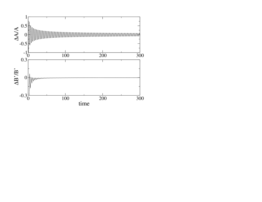
Figure 1: The fractional difference between the asymptotic value and the finite time value of the expressions in eqs.(18) and (19). The quantities $\Delta A$ and $\Delta B^{\prime}$ are defined in the text.

3.3 Generalized quantum walk

In this subsection we present an alternative analytical approach which can be applied to the generalized quantum walk, i.e. for arbitrary values of $\theta$. We start by rearranging the original map, eqs.(4), to uncouple both chirality components. The resulting independent evolution equations are

$$a_{i}(t+2)-a_{i}(t) =\cos\theta\,\left[a_{i+1}(t+1)-a_{i-1}(t+1)\right]$$

$$b_{i}(t+2)-b_{i}(t) =\cos\theta\,\left[b_{i+1}(t+1)-b_{i-1}(t+1)\right].$$ (23)

For long times the left hand sides of the above equations can be approximated by time derivatives. The result can be expressed as

$$2\frac{\partial\xi_{i}}{\partial t}=\cos\theta\left[\xi_{i+1}(t)-\xi_{i-1}(t)\right],$$ (24)

where $\xi_{i}$ stands for either chirality component, $a_{i}$ or $b_{i}$. We define the effective time $t^{\prime}=-t\,cos\theta$, then eq.(24) becomes

$$2\frac{\partial\xi_{i}}{\partial t^{\prime}}=\xi_{i-1}(t^{\prime})-\xi_{i+1}(t^{\prime}),$$ (25)

which is the recursion relation satisfied by the Bessel functions. Thus, we can write the general solution as

$$\xi_{i}(t)=\sum_{-\infty}^{+\infty}(-1)^{i-l}\tilde{\xi}_{l}(0)J_{i-l}(t\,\cos\theta),$$ (26)

where $\tilde{\xi}_{l}(0)$ are the initial conditions to be used in the differential equation (25). These initial conditions are not necessarily the same as those to be used in the discrete map (23), because the approximation of a difference by a continuous derivative does not hold for small times. The solution (26) with appropriate initial conditions provides a good long–time description of the dynamics of the discrete map (23). In this context, long–time implies many applications of the discrete map. Note that eq.(26) provides the additional information [6] that the long–time propagation speed of the probability distribution is given by $\cos\theta$.

It is worth mentioning that the long–time solutions for the spinor amplitudes, eq.(26), have the same form as the time-evolution of the amplitudes of the kicked rotor in a principal resonance [15, 16]. In fact, if $K$ is the dimensionless strength parameter of the kicked rotor as defined in [17], the time evolution for these amplitudes is given by eq.(26) after the substitution

$$\cos\theta\rightarrow\frac{K}{4\pi p}\qquad\qquad\mbox{{p}\;\;\;integer}.$$ (27)

Figure 2: Fractional difference between the variance as obtained from the approximate expressions (29) and (30), and the exact value $\sigma^{2}$ from the original Hadamard map, eq.(4). The quantity $\Delta\sigma^{2}$ is defined in the text. The initial conditions used in eqs.(29) and (30) are ${\binom{\tilde{a}_{0}}{\tilde{b}_{0}}}=0.70206{\binom{1}{1}}$, ${\binom{\tilde{a}_{\pm 2}}{\tilde{b}_{\pm 2}}}=-0.05963{\binom{1}{1}}$ and zero otherwise. For the calculation of $\sigma^{2}$, the particle is initially at the origin with chirality ${\binom{a_{0}}{b_{0}}}={\binom{1}{0}}$.

We can obtain analytically the increase in the variance implied by eq.(26). The position probability distribution can be expressed as

$$P_{i}(t)=\sum_{l,l^{\prime}}(-1)^{-(l+l^{\prime})}\left[\tilde{a}_{l}(0)\tilde{a}_{l^{\prime}}^{\ast}(0)+\tilde{b}_{l}(0)\tilde{b}_{l^{\prime}}^{\ast}(0)\right]\,J_{i-l}(t\cos\theta)\,J_{i-l}^{\prime}(t\cos\theta).$$ (28)

The first and second moments of this distribution are

$$M_{1}(t)=-t\,\cos\theta\,\sum_{l}\Re\left[\tilde{a}_{l}(0)\tilde{a}_{l-1}^{\ast}(0)+\tilde{b}_{l}(0)\tilde{b}_{l-1}^{\ast}(0)\right]+M_{1}(0)$$ (29)

and

$$M_{2}(t) =\frac{t^{2}\cos^{2}\theta}{2}\left\{1+\sum_{l}\Re\left[\tilde{a}_{l}(0)\tilde{a}_{l-2}^{\ast}(0)+\tilde{b}_{l}(0)\tilde{b}_{l-2}^{\ast}(0)\right]\right\}$$

$$\qquad-t\,\cos\theta\,\sum_{l}(2l-1)\Re\left[\tilde{a}_{l}(0)\tilde{a}_{l-1}^{\ast}(0)+\tilde{b}_{l}(0)\tilde{b}_{l-1}^{\ast}(0)\right]+M_{2}(0).$$ (30)

respectively, where $M_{1}(0)$ and $M_{2}(0)$ are the moments of the initial distribution. Thus the variance $\sigma^{2}=M_{2}-M_{1}^{2}$ increases quadratically in time for arbitrary initial conditions. This result holds for arbitrary (non–trivial) values of the parameter $\theta$. In Fig. 2 we show the time evolution of the relative difference $\Delta\sigma^{2}/\sigma^{2}$ where $\Delta\sigma^{2}\equiv\sigma^{2}_{ap}-\sigma^{2}$ is the difference between the approximate variance $\sigma^{2}_{ap}$ obtained from eqs.(29) and (30) and the exact variance $\sigma^{2}$ from the original Hadamard map, eq.(4).

The independence of the quadratic increase of $\sigma^{2}$ on the initial conditions has been established numerically for the particular case of the Hadamard walk [14]. Here we have also demonstrated the independence of this quadratic increase on the parameter of the unitary transformation. This is a new result.

4 Conclusions

The quadratic increase in time of the variance for the discrete time generalized quantum walk has been obtained analytically. This increase remains quadratic for arbitrary initial conditions and for all non–trivial values of the parameter $\theta$ controlling the unitary transformation in the chirality subspace. This quadratic increase results from interference effects and thus it is strongly dependent on the coherence of the quantum evolution. If, for any reason, the quantum evolution is decoherent then the increase in the variance becomes linear with time.

The general approach of separating the quantum evolution equation into a master equation supplemented by a term which takes into account quantum coherence effects provides a new perspective which is helpful in clarifying why the quantum evolution spreads faster than in the classical one. In the quantum case, there is a superposition of a left-propagating wave and a right-propagating wave, with both wavefronts traveling with constant speed $\cos\theta$. Thus, their separation increases linearly in time and the variance does so quadratically. In the Markovian approximation, as developed in this work, the particle moves a step either to the right or to the left, making its choice in a random way. Due to the randomness of this motion, the variance increases only linearly with time. This process can be visualized as a frequent position measurement process, which amounts to reinitialize the system, at each measurement, in a different state. The wave function collapse causes memory loss of the previous distribution. Thus, we have a Markovian process which describes a series of random steps.

We have shown how the Markovian approximation method can be applied to a generalized quantum walk, for arbitrary values of the parameter $\theta$ and arbitrary initial conditions. When the evolution becomes decoherent, the interference terms may be dropped and the evolution is described by a master equation implying a linear increase of the variance with time. The diffusion coefficient is not, in general, the same as that for the classical random walk. Only in the particular case of the Hadamard walk the diffusion coefficient is $1/2$ as in the classical case. This formalism shows in a transparent form that the primary effect of decoherence is to make the interference terms negligible in the evolution equation and then the Markovian behavior is immediately implied. This is true for any evolution operator of the form given in eq.(1).

We have established the analogy between the generalized quantum walk and the resonant kicked rotor. This is done by obtaining an expression for the time evolution of the chirality amplitudes of the quantum walk and showing that they have the same form as the angular momentum components of the wavefunction of the kicked rotor in a resonant regime. We related the kicked rotor strength parameter to the parameter $\theta$ defining the unitary transformation of the chirality. This analogy opens several interesting possibilities. A quantum algorithm implements the evolution of the quantum kicked rotor in a quantum computer is known [18]. Since the quantum random walk on the line has the same long–time dynamics as the resonant kicked rotor, the same quantum algorithm may be used to describe the evolution of a generalized discrete time quantum walk on the line. The quantum kicked rotor has been experimentally realized using ultra-cold atom traps and some experiments have focused on the resonant case [19]. This opens interesting possibilities for the experimental realization of the quantum walk using quantum optics.

Finally, note that the Markovian approach presented here provides a systematic way to find the classical analog associated to a given quantum random walk. By reformulating the quantum problem as described here and neglecting the interference terms, the Markovian equation describing the equivalent classical problem can be readily obtained.

We acknowledge the comments made by V. Micenmacher and the support of PEDECIBA and CONICYT (Clemente Estable proy. 6026) . R.D. acknowledges partial financial support from the Brazilian Research Council (CNPq). A.R, G.A. and R.D. acknowledge financial support from the Brazilian Millennium Institute for Quantum Information–CNPq.

References

- [1] R. Feynman, Int. J. Theor. Phys. 21, 467 (1982).
- [2] M. Nielssen and I. Chuang, Quantum Computation and Quantum Information, Cambridge University Press, 2000.
- [3] P. Shor, Proceedings of the 35th Annual Symposium on Foundations of Computer Science,p. 124, IEEE Computer Society Press, Los Alamitos, CA, 1994; arXiv:SIAM J. Comp., 26, 1484 (1997).
- [4] L.K. Grover, Phys. Rev. Lett. 79, 325 (1997).
- [5] A. Nayak and A. Vishwanath, preprint arXiv:quant-ph/0010117.
- [6] A. Childs, E. Farhi, S. Gutmann, Quantum Information Processing, 1, 35 (2002); preprint arXiv:quant-ph/0103020.
- [7] J. Kempe, Contemporary Physics, 44, 307 (2003); preprint arXiv:quant-ph/0303081.
- [8] B. Tregenna, W. Flanagan, R. Maile and V. Kendon, New J. Phys. 5 (2003) 83; preprint arXiv:quant-ph/0304204.
- [9] E. Bach, S. Coppersmith, M. Paz Goldschen, R. Joynt, J. Watrous, preprint arXiv:quant-ph/0207008.
- [10] A. Romanelli, A.C. Sicardi-Schifino, G. Abal, R. Siri, R. Donangelo. Phys. Lett. A, 313, 325 (2003); preprint arXiv:quant-ph/0204135.
- [11] Salvador Godoy and L.S. García-Colín. Phys. Rev. E 53, 5779 (1996).
- [12] S.Goldstein Quart.Journ. Mech. and Applied Math IV, 129 (1951).
- [13] N. Konno, Quantum Information Processing, 1, 345 (2002); preprint arXiv:quant-ph/0206053.
- [14] B. Travaglione and G. Milburn, Phys. Rev. A 65, 032310, (2002).
- [15] F. M. Izrailev, Phys. Rep. 196, 299 (1990).
- [16] F.M. Izrailev and D.L. Shepelyankii, Theor. Math. Phys. 43 553 (1980).
- [17] G. Abal, R. Donangelo, A. Romanelli, A.C. Sicardi-Schifino and R. Siri, Phys. Rev. E 65, 046236 (2002).
- [18] B. Georgeot and D. L. Shepelyansky. Phys. Rev. Lett. 86, 2890 (2001).
- [19] M.E.K. Williams, M.P. Sadgrove, A.J.Daley, R.N.C. Gray, S.M. Tan, A.S. Parkins and R. Leonhardt, preprint arXiv:quant-ph/0209090 (2002); F.L. Moore, J.C. Robinson, C.F. Bharucha B. Sundaram and M.G. Raizen, Phys. Rev. Lett. 75 4598 (1995).