Thermal entanglement of Bosonic atoms in an optical lattices with nonlinear couplings

Abstract

The thermal entanglement of two spin-1 atoms with nonlinear couplings in an optical lattices is investigated in this paper. It is found that the nonlinear couplings favor the thermal entanglement creating. The dependence of the thermal entanglement in this system on the linear coupling, the nonlinear coupling, the magnetic field and temperature is also presented. The results show that the nonlinear couplings really change the feature of the thermal entanglement in the system, increasing the nonlinear coupling constant increases the critical magnetic field and the threshold temperature.

Entanglement as a valuable resource for quantum information processing (QIP) bennett ; nielsen1 ; plenio1 has attracted a lot of attention in recent years, from both experimental and theoretical studies raimond . Since the entanglement is fragile, the problem of how to create stable entanglement remains a main focus of recent studies in the field of quantum information processing. The thermal entanglement, which differs from the other kind of entanglement by its advantages of stability, requires neither measurement nor controlled switching of interactions in the preparation process, hence the thermal entanglement in various systems is an attractive topic and worth intensively studying.

The system of atoms in optical lattices is among the promising candidates for quantum information processing. It may take the advantage of the technology used in atom optics and laser cooling based on the optical manipulation of atoms birkl . Besides, it also holds the merit of eventual possibility to scale, parallelize and miniaturize the device in QIP.

The thermal entanglement has been extensively studied for various systems including isotropic Heisenberg chain arnesen ; oconnor ; iso , anisotropic Hensenberg chain aniso , Ising model in an arbitrarily directed magnetic field ising , and cavity-QED cqed since the seminal works by Arnesen et al. arnesen and Nielsen nielsen2 . Based on the tools developed within the context of quantum information theory, the relaxation of a quantum system towards the thermal equilibrium is investigated scarani , which provides us a different mechanism to model a system arriving at the thermal entangled states. For a specific Heisenberg chain in condensed matter physics, the only ranging variables are the magnetic field and the temperature arnesen , in cavity-QED system, the exchange constant (the linear coupling in our case) is adjustable in addition to the temperature and magnetic field. The development of laser cooling and trapping provides us more ways to control the atoms in traps. Indeed, we can manipulate the atom-atom coupling constants and the atom number in each lattice well with a very well accuracy greiner ; yip .

In this paper, we study the thermal entanglement in optical lattice with nonlinear couplings. We calculate the thermal entanglement as a function of the nonlinear coupling constant, linear coupling constant, the temperature as well as the external magnetic field. We will confine ourself in this paper to the case of $K<0$ and $J<0$ that is relevant to the recent experiment conducted on ${}^{23}Na$ atoms. As we will show you later on, there is no thermal entanglement in the regime of $K>J$ when $J<0$ similar to the results for the isotropic Heisenberg model arnesen . Our studies also show that the critical magnetic field and the threshold temperature is obviously increased by the presence of the nonlinear couplings.

Our system consists of two wells in the optical lattice with one spin-1 atom in each well. The lattice may be formed by three orthogonal laser beam, and we may use an effective Hamiltonian of the Bose-Hubbard form jaksch to describe the system. The atoms in the Mott regime make sure that each well contains only one atom. For finite but small hopping term $t$, we can expand the Hamiltonian into powers of $t$ and get yip ,

$$H=\epsilon+J(\vec{S}_{1}\cdot\vec{S}_{2})+K(\vec{S}_{1}\cdot\vec{S}_{2})^{2},$$ (1)

where $J=-\frac{2t^{2}}{U_{2}},K=-\frac{2t^{2}}{3U_{2}}-\frac{4t^{2}}{U_{0}}$ with $t$ the hopping matrix elements, and $\epsilon=J-K$. $U_{s}$ ($s=0,2)$ represents the Hubbard repulsion potential with total spin $s$, a potential $U_{s}$ with $s=1$ is not allowed due to the identity of the bosons with one orbital state per well, $\vec{S}_{i}(i=1,2)$ denote the spin vector $\vec{S}_{i}=(S_{ix},S_{iy,}S_{iz})$. This Hamiltonian differs from the usual Heisenberg model by the nonlinear couplings. Since term $\epsilon$ contains no interaction, we can ignore it in the following discussions and it would not change the thermal entanglement. In the presence of external magnetic field, the Hamiltonian Eq. (1) becomes

$$H=J(\vec{S}_{1}\cdot\vec{S}_{2})+K(\vec{S}_{1}\cdot\vec{S}_{2})^{2}+B(S_{1z}+S_{2Z}),$$ (2)

where the magnetic field $\vec{B}$ along the z-direction is assumed. When the total spin for each site $S_{i}=1(i=1,2)$, its components take the form

$$S_{ix}=\frac{1}{\sqrt{2}}\left(\begin{array}[]{ccc}0&1&0\\ 1&0&1\\ 0&1&0\end{array}\right),S_{iy}=\frac{1}{\sqrt{2}}\left(\begin{array}[]{ccc}0&-i&0\\ i&0&-i\\ 0&i&0\end{array}\right),S_{iz}=\left(\begin{array}[]{ccc}1&0&0\\ 0&0&0\\ 0&0&-1\end{array}\right).$$ (3)

The ground state of Hamiltonian Eq.(2) is expected to be the dimer phases, as the most recently study yip conclude, this is quite different from the Heisenberg chain without nonlinear couplings. And the nonlinear couplings would make the thermal entanglement different from that in the usual Heisenberg model, too, as you will see.

To get the thermal entanglement, we first present the eigenvalues and the corresponding eigenstates of the Hamiltonian Eq.(2),

$$E_{1} = K+J-B;|\Psi_{1}\rangle=\frac{1}{\sqrt{2}}(|0,-1\rangle+|-1,0\rangle),$$

$$E_{2} = K+J+B;|\Psi_{2}\rangle=\frac{1}{\sqrt{2}}(|1,0\rangle+|0,1\rangle),$$

$$E_{3} = K-J+B;|\Psi_{3}\rangle=\frac{1}{\sqrt{2}}(-|1,0\rangle+|0,1\rangle),$$

$$E_{4} = K-J-B;|\Psi_{4}\rangle=\frac{1}{\sqrt{2}}(-|0,-1\rangle+|-1,0\rangle),$$

$$E_{5} = K+J;|\Psi_{5}\rangle=\frac{1}{\sqrt{6}}(|1,-1\rangle+|-1,1\rangle+2|0,0\rangle),$$

$$E_{6} = K-J;|\Psi_{6}\rangle=\frac{1}{\sqrt{2}}(|1,-1\rangle-|-1,1\rangle),$$

$$E_{7} = K+J+2B;|\Psi_{7}\rangle=|1,1\rangle,$$

$$E_{8} = K+J-2B;|\Psi_{8}\rangle=|-1,-1\rangle,$$

$$E_{9} = 4K-2J;|\Psi_{9}\rangle=\frac{1}{\sqrt{3}}(|1,-1\rangle+|-1,1\rangle-|0,0\rangle).$$

The state of the above system at thermal equilibrium is $\rho=Z^{-1}\exp(-\beta H)$, where $Z=Tr[\exp(-\beta H]$ is the partition function and $\beta=1$ $/k_{B}T$ ($k_{B}$ is Boltzmann’s constant. For simplicity we will set $k_{B}=1$ hereafter). In terms of the eigenstates and the corresponding eigenvalues, the state of the system can be expressed as

$$\rho=\frac{1}{Z}\sum_{i=1}^{9}e^{-\beta E_{i}}|\Psi_{i}\rangle\langle\Psi_{i}|$$ (5)

with the partition function

$$Z=2e^{-\beta K}\cosh(\beta B)(1+2\cosh(\beta J))+2e^{-\beta(K+J)}\cosh(2\beta B)+e^{-\beta(4K-2J)}.$$ (6)

We will choose the negativity as the entanglement measure vidal ,

$$N(\rho)=\frac{\left\|\rho^{T_{A}}\right\|-1}{2},$$ (7)

where $\left\|\rho^{T_{A}}\right\|$ denotes the trace norm of the partial transpose $\rho^{T_{A}}$. The negativity $N(\rho)$ is equivalent to the absolute value of the sum of the negative eigenvalues of $\rho^{T_{A}}$horodecki . Although the negativity lacks a direct physical interpretation, it bounds two relevant quantities in quantum information processing–the channel capacity and the distillable entanglement. As the negativity is a computable measure of entanglement for bipartite system with any dimension, we here choose it to measure the thermal entanglement.

We have performed extensive numerical calculations for the entanglement measure, some selected results are presented in figures from 1 to 3.

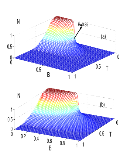
Figure 1: (Color on line) The thermal entanglement vs. the external magnetic field $B$ and temperature. We choose the negativity as the entanglement measure, $B$ and $T$ are plotted in units of the Boltzmann’s constant $k_{B}$. At $T=0$, $N$ has a sharp transition from 1 to 0 as $B$ crosses the critical value of $B=3/2(J-K)$. The $B=0.35$ line pointed out in the figure shows that for certain value of $B$ it is possible to increase $N$ by increasing temperature $T$. Figure 1-(a), (b) are for different $K$, (a) $K=-0.6$ and (b) $K=-0.7$.

Figure 1 shows the plot of the negativity as a function of the magnetic field $B$ and temperature $T$. For $B=0$, the state $|\Psi_{9}\rangle$ is the ground state exp , and the others in Eq. (LABEL:eigen) are excite states. In this case, the maximal entanglement is at $T=0$ and it decreases with $T$ due to mixing of the excited states with the ground state. For a higher value of $B$ greater than $B_{c}=3/2(J-K)$, $|\Psi_{8}\rangle$ becomes the ground state. In that case, there is no entanglement at $T=0$, but we may increase the entanglement by increasing $T$, that is to bring entangled eigenstates such as $|\Psi_{i}\rangle$ $(i=1,2,3,4,5,6,9)$ into mixing with the ground state. It is interesting to note that the critical field $B_{c}$ depends on both the linear coupling $J$ and the nonlinear coupling $K$. With $K=0$, $B_{c}$ gives rise to $3/2J$ that means no entanglement in this case (i.e. for $J<0$) at any temperature and with any values of magnetic field. We would like to address that $J$, $K$ and $B$ together determine the ground state properties of the system instead of $J$ and $B$ in the isotropic Heisenberg model. This is a quite different feature from the previous studies. For example, we may choose $K$, $J$ and $B$ such that $|\Psi_{1}\rangle$ is the ground state of the system, it is entangled state but not a maximally entangled one. The critical magnetic field can be increased by increasing the nonlinear coupling $|K|$, as shown in figure 1-(b), where the entanglement is plotted as a function of $T$ and $B$ with the same parameters as in figure 1-(a), but $K=-0.7$. It is obvious that the threshold temperature above which the entanglement vanishes has also been increased. More clearly, this point was shown in figure 2, where we plot the thermal entanglement in the system as a function of $K$ and $T$.

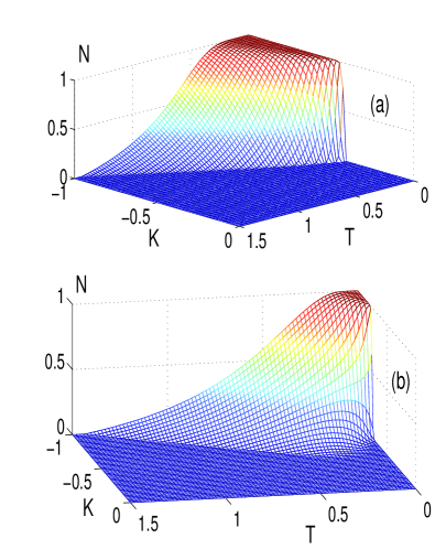
Figure 2: (Color on line) This figure depicts the thermal entanglement as a function of the temperature $T$ and the nonlinear coupling constant $K$ with a specific $J=-0.4$. The degree of entanglement is measured in terms of the negativity. Figure 2-(a), (b) are for different $B$, (a) $B=0$, and (b) $B=0.5$. All parameters are re-scaled in units of $k_{B}$.

For $B=0$, the thermal entanglement is not zero only for $|K|>0.4$, as the figure 2-(a) shows, this indicates that $|K|>|J|$ is a necessary condition for thermal entanglement to exist. Further analysis shows that for $B=0$ and with a specific temperature $T$ the condition for thermal entanglement to exist is

$$K<J-\frac{T}{3}ln(\frac{5+3e^{2J/T}}{2}).$$ (8)

The condition Eq.(8) also holds for $J>0$ and $K>0$, since we made no constraint on the derivation of Eq.(8). On the other hand, it gives rise to a analytical expression for the threshold temperature $T_{c}$ in the case of $B=0$ by solving $K=J-\frac{T_{c}}{3}ln(\frac{5+3e^{2J/T_{c}}}{2})$, it shows again that $T_{c}$ depends on $J$ and $K$. In addition to the above feature, there is a evidence that the threshold temperature is a monotonous function of $|K|$ with $B=0$, the larger the nonlinear coupling constant $|K|$, the larger the threshold temperature. This point would be changed when the magnetic field is present (Fig. 2-(b)), as you see the threshold temperature is no longer a monotonous function of $|K|$. We now look at the dependence of the thermal entanglement on $J$ and $K$, with a fixed $B$ and $T$, the selected results for this dependence were illustrated in figure 3. As figure 3 shows, the thermal entanglement may exist only in the regime of larger $|K|$, or smaller $|J|$.

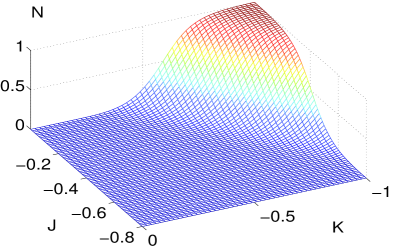
Figure 3: (Color on line) Thermal entanglement vs. the coupling constants $J$ and $K$. The selected results are chosen from the regime of $J,K<0$, which is relevant to atoms ${}^{23}Na$ in an optical lattice. The parameters chosen are $B=0.8$ and $T=0.2$. All parameters are rescaled in units of $k_{B}$, the Boltzmann’s constant.

Now we discuss the experimental feasibility for observing the thermal entanglement in the optical lattice. We may choose ${}^{23}Na$ trapped in an optical lattice as the system. Bose-Einstein condensates of unpolarized ${}^{23}Na$ have already been achieved by the MIT group stenger . The ${}^{23}Na$ atoms have hyperfine spin 1, and the interaction among them is antiferromagnetic ($t>0$) that is essential for the thermal entanglement to exist in isotropic Heisenberg model. There are two parameters, the hopping matrix $t$ and the Hubbard repulsion $U_{2}$ (or $U_{0}$), we may control separately by adjusting the strength of the sinusoidal potentials via the intensities of the laser beams, the coupling constants for the linear interaction $J$ and the nonlinear term are hence adjustable. The two wells in the optical lattice in question can be isolated by increasing the barriers connecting to the other wells in the optical lattice. With these done, the two ${}^{23}Na$ atoms in the Mott regime then end up in a thermal entangled state.

To conclude, we have studied the thermal entanglement in a optical lattice, the dependence of the thermal entanglement measured by the negativity on the linear coupling constant $J$, the nonlinear coupling constant $K$, the external magnetic field and temperature was presented and discussed. There are two different points in contract to the isotropic Heisenberg model, one is the dimensionality and another is the nonlinearity of the couplings. When the nonlinear coupling is zero, there is no thermal entanglement in the regime $J>0$, this is similar to that in the isotropic Heisenberg model in spite of different dimensionality. The nonlinear coupling really change the feature of the thermal entanglement, increasing $|K|$ increases the critical magnetic field and the threshold temperature. The thermal entanglement in an optical lattice with more than two coupled wells remains untouched. In future, we will investigate these problems and study how to map this natural entanglement onto photons and use it as a resource in QIP.

This work was supported by EYTP of M.O.E, and NSF of China.

References

- (1) C. H. Bennett and D. P. DiVincenzo, Nature 404, 247(2000).
- (2) M. A. Nielsen and I. L. Chuang, Quantum computation and quantum information (Cambridge University press, Cambridge, 2000).
- (3) M. B. Plenio and V. Vedral, Contemp. Phys. 39,431(1998).
- (4) See, for example, J. M. Raimond et al., Rev. Mod. Phys. 73, 565(2001); Vedral, Rev. Mod. Phys. 74, 197(2002).
- (5) G. Birkl et al., Optics Comm. 191, 67 (2001).
- (6) M. C. Arnesen, S. Bose and V. Vedral, Phys. Rev. Lett. 87, 017901 (2001).
- (7) K. M. OConnor and W. K.Wootters, Phys. Rev. A 63, 052302 (2001).
- (8) X. Wang, Phys. Rev. A 66 ,044305 (2002); X. Wang, Phys. Rev. A 66 , 034302 (2002).
- (9) X. Wang, Phys. Rev. A 64 , 012313 (2001);G. L. Kamta and A. F. Starace, Phys. Rev. Lett. 88, 107901(2002);L. Zhou, H. S. Song, Y. Q. Guo and C. Li, Phys. Rev. A 68, 024301 (2003).
- (10) D. Gunlycke et al., Phys. Rev. A 64, 042302 (2001).
- (11) S. Mancini, and S. Bose, e-print quant-ph/0111055.
- (12) M. A. Nielsen, e-print quant-ph/0011036.
- (13) V. Scarani et al., Phys. Rev. Lett. 88, 097905 (2002).
- (14) M. Greiner et al., Nature London 415, 39(2002).
- (15) S. K. Yip, Phys. Rev. Lett. 90, 250402 (2003).
- (16) D. Jaksch, C. Bruder, J.I. Cirac, C. W. Gardiner, and P. Zoller, Phys. Rev. Lett. 81,3108 (1998).
- (17) G. Vidal, R. F. Werner, Phys. Rev. A 65, 032314 (2002).
- (18) K. Zyczkowski, P. Horodecki et al, Phys. Rev. A 58, 883(1998).
- (19) It depends on the parameters and chosen. For an optical lattice with atoms, it is shown that .
- (20) J. Stenger et al., Nature (London) 396, 245 (1999).