Two independent photon pairs versus four-photon entangled states in parametric down conversion

Abstract

We study the physics of four-photon states generated in spontaneous parametric down-conversion with a pulsed pump field. In the limit where the coherence time of the photons $t_{c}^{ph}$ is much shorter than the duration of the pump pulse $\Delta t$, the four photons can be described as two independent pairs. In the opposite limit, the four photons are in a four-particle entangled state. Any intermediate case can be characterized by a single parameter $\chi$, which is a function of $t_{c}^{ph}/\Delta t$. We present a direct measurement of $\chi$ through a simple experimental setup. The full theoretical analysis is also provided.

I Introduction

Spontaneous parametric down-conversion (SPDC) mandel ; walls is a light amplification process that takes place in a non-linear $\chi^{2}$ medium, where a photon from a pump field is converted into two photons, usually called signal and idler, with energy and momentum conservation. The signal and idler fields are therefore strongly correlated in energy, emission times, polarization and momentum. SPDC is a very convenient tool to produce entangled states of photons, which have been used to test the foundation of quantum physics and are at the heart of quantum information processing and communications (see tw for a review). In the basic setup, the pump field is cw, and the output state is the so-called two mode squeezed state (see e.g. walls Eq. (5.64)). When the pump intensity is low enough, the output state is well described by a large vacuum component plus a two-photon state, a photon pair. Recently, physicist have started to go beyond this basic configuration. On the one hand, when the classical pump field is no longer cw but pulsed. In this case, the down-conversion process can take place only when a pump pulse is ”inside” the crystal, thus providing an information about the time at which the down-converted photons are emitted. Of course, as a counterpart, coherence is lost in the frequency domain, since a pulsed pump field is not monochromatic. Non-trivial effects of a pulsed pump have been predicted keller ; grice and observed exper for photon pairs. On the other hand, more efficient sources and large pump intensities allow to produce an output field where the four -and more- photons components are longer negligible. The four-photon component of the field is of interest in quantum optics wang and in quantum information, since four-qubit entanglement can be obtained wein ; howell02 ; Eibl 03 . But this component can be a nuisance as well, for instance in quantum teleportation, because its presence decreases the fidelity of the two-qubit Bell state measurement HDR03 or in two-photon interference experiments where it limits the visibility marcikic02 .

In this paper, we investigate both experimentally and theoretically the physics of the four-photon component produced in down-conversion, with a pulsed pump field. We start with a qualitative description of what is to be expected. The two meaningful quantities are the duration of the pump pulse $\Delta t$ and the coherence time of the observed down-converted photons $t_{c}^{ph}$. The characteristics of the four-photon state are captured by the relation between $P_{2}$ and $P_{4}$, the probabilities of creating 2, resp. 4 photons.

Let us consider first the limit $t_{c}^{ph}\ll\Delta t$. A large number of independent SPDC processes can take place inside a pump pulse comment1 . In this limit, any $2n$ photon state can be satisfactorily described as n independent pairs. The probability of creating $n$ pairs in a given pulse is described according to a Poisson distribution of mean value $\mu$ $P_{n}=e^{-\mu}\mu^{n}/n!$, as shown in Section II. In particular, for small $\mu$ we have $P_{4}\approx\frac{P_{2}^{2}}{2}$, and the four-photon state corresponds to two independent pairs, labelled $|2\mbox{ EPR}\rangle$.

The other limit, $t_{c}^{ph}\gg\Delta t$, can be achieved by the use of femtosecond pump pulses and narrow filtering of signal and idler photons. This condition is mandatory for all experiments where photons created in different SPDC events must interfere at a beam splitter, in order to preserve the temporal indistinguishability zukowski95 . In this case, the emission of a ”second pair” is stimulated by the presence of the first one Lamas01 leading to an entangled four-photon state $|4\mbox{ entg}\rangle$ that cannot be described as two independent pairs. Because of stimulated emission, we have $P_{4}={P_{2}}^{2}$.

In the present paper, we study the transition between these two extreme situations. We define a parameter $\chi\in[0,1]$ that allows to interpolate between the Poisson distribution and the statistics arising from stimulated emission according to

$$P_{4} = \frac{{P_{2}}^{2}}{2}(1+\chi)\,.$$ (1)

In Section II, we present an intuitive description of the physics in the language of quantum states. In Section III, we present a simple experiment that allows to measure $\chi$. In Section IV, we give the full quantum-optical formalism to describe the four-photon component of the field, and work out an approximate solution which agrees well with the experimental data. In particular, we find that $\chi$ depends on $t_{c}^{ph}$ and $\Delta t$ only through their ratio

$$r = t_{c}^{ph}/\Delta t\,.$$ (2)

II The four-photon state

A coherent down-conversion process produces the two-mode squeezed state

$$|\Psi\rangle = \sum_{n}\frac{T^{n}}{C}\,\mbox{$|n;n\rangle$}$$ (3)

where $T\equiv\tanh\xi$ and $C\equiv\cosh\xi$ and $\xi$ is proportional to the amplitude of the pump field (see walls Eq. (5.64)). The state $|n;n\rangle$ describes the field with $n$ photons in the signal mode and $n$ photons in the idler mode; in particular, $\mbox{$|2;2\rangle$}\equiv\mbox{$|4\mbox{ entg}\rangle$}$ is the four-photon state described in the introduction.

In the limit where we study photons whose coherence is much larger than the time-bin (the width of the pump pulse), that is $t_{c}^{ph}\gg\Delta t$, there is a unique coherent down-conversion process taking place in the crystal for each pump pulse, and in this case the four-photon component of the field is $|4\mbox{ entg}\rangle$. We expect $\chi=1$.

If $t_{c}^{ph}<\Delta t$, a number $N\approx\Delta t/t_{c}^{ph}=1/r$ of independent SPDC processes can take place inside a pump pulse. To simplify this discussion, we consider $N$ as an integer. The state of the field reads then

$$\mbox{$|\Psi\rangle$}^{\otimes N} = \frac{1}{C^{N}}\,\sum_{n}T^{n}\,\mbox{$|2n\rangle$}\,=\,\frac{1}{C^{N}}\,\big{(}\mbox{$|0\rangle$}+T\mbox{$|2\rangle$}+T^{2}\mbox{$|4\rangle$}+...\big{)}\,,$$ (4)

where the $|2n\rangle$ is the un-normalized superposition of all the states containing $2n$ photons. Specifically:

The two-photon component $|2\rangle$ is the sum of the $N$ states that describe ”one pair in process $j$ and no pairs in the other processes”, that is $\mbox{$|2\rangle$}=\mbox{$|1;1\rangle$}\otimes\mbox{$|0\rangle$}...\otimes\mbox{$|0\rangle$}\,+\,...\,+\,\mbox{$|0\rangle$}\otimes\mbox{$|0\rangle$}...\otimes\mbox{$|1;1\rangle$}$. Since all the components are mutually orthogonal, we have $\mbox{$\langle 2|2\rangle$}=N$. The four-photon component $|4\rangle$ is the sum of two kind of terms: (i) The $N$ components $\mbox{$|2;2\rangle$}\otimes\mbox{$|0\rangle$}\cdots\otimes\mbox{$|0\rangle$}+\mbox{$|0\rangle$}\otimes\mbox{$|0\rangle$}\cdots\otimes\mbox{$|2;2\rangle$}$, in which the second pair is created by stimulated emission; each of these gives rise to the correlations of $|4\mbox{ entg}\rangle$. (ii) The $N(N-1)/2$ components where one pair is produced in process $j$ and another pair is produced in a different process $j\,^{\prime}$. Each of these gives rise to the correlations of $|2\mbox{ EPR}\rangle$. Therefore $\mbox{$\langle 4|4\rangle$}=N(N+1)/2$, and by normalizing this component we can say that the ”four-photon state” is

$$|\Psi_{4}(N)\rangle = \sqrt{\frac{2}{N+1}}\,\mbox{$|4\mbox{ entg}\rangle$}\,+\,\sqrt{\frac{N-1}{N+1}}\,\mbox{$|2\mbox{ EPR}\rangle$}\,.$$ (5)

Referring back to (4), we can compute the probabilities of having two or four photon: $P_{2}(N)\,=\,\frac{1}{C^{2N}}\,T^{2}\,N$, $P_{4}(N)\,=\,\frac{1}{C^{2N}}\,T^{4}\,\frac{N(N+1)}{2}$. In the limit of very large number of independent processes $N$, the usual argument leads to the Poisson distribution notepoiss . Now we have all the elements to compute $\chi$ and relate it to the description of the four-photon component. For simplicity, we put $C=1$. Then from (1) we obtain $\chi=2P_{4}(N)/P_{2}(N)^{2}-1$ that is

$$\chi\,=\,\frac{1}{N}\,=r t_{c}^{ph}<<\Delta t$$ for (6)

and we can re-write the four-photon state as

$$|\Psi_{4}(\chi)\rangle = \sqrt{\frac{2\chi}{1+\chi}}\,\mbox{$|4\mbox{ entg}\rangle$}\,+\,\sqrt{\frac{1-\chi}{1+\chi}}\,\mbox{$|2\mbox{ EPR}\rangle$}\,.$$ (7)

This provides an intuition on the link between $\chi$, the experimental parameter $r$ and the entanglement in the four-photon state.

III The experiment

A schematic of the experiment that measures $\chi$ is shown in Fig. 1.

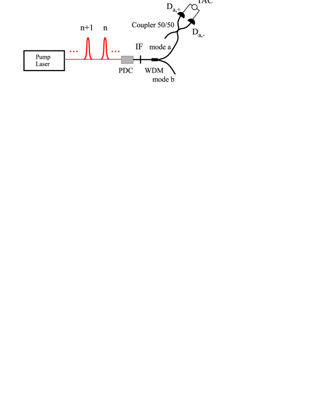
Figure 1: Schematic of the experiment used to measure the stimulation parameter $\chi$. See text for details.

A non-degenerate type I parametric down-converter is pumped by a pulsed laser. PDC modes $a$ and $b$ are then separated deterministically, via their different wavelengths. We ignore photons in mode $b$; in mode $a$, we detect coincidence counts between the outcomes of a passive coupler. This coincidence measurement post-selects the events in which at least four photons have been produced in the down-conversion processes. The idea is to compare the events where four photons are created in the same pump pulse with the events where one pair is created in one pulse and another one in the next pulse. In the first case, we detect a coincidence in a time window centered at $\Delta t_{det}=0$. The coincidence count rate $R_{0}$ of this peak is proportional to $\frac{1}{2}P_{4}$. The factor $\frac{1}{2}$ is the probability that the two photons exit different modes of the beam splitter. In the second case, we detect a coincidence with $\Delta t_{det}=\Delta\tau_{laser}$ (time between 2 laser pulses). We restrict ourself to the case when a photon created in pulse n is detected by detector $D_{a,+}$ while photon created in pulse $n+1$ is detected by detector $D_{a,-}$. The coincidence count rate $R_{side}$ is thus proportional to $\frac{1}{4}[P_{2}(I)]^{2}$. Consequently, we have

$$\frac{R_{0}}{R_{side}}=\frac{2P_{4}}{[P_{2}]^{2}}=\chi+1.$$ (8)

Here is a description of the experimental setup. A mode-locked femto-second laser, generating Fourier transform limited pulses at 710 nm, is used to pump a lithium triborate (LBO) type I non linear crystal. The time between two subsequent laser pulses is $\Delta\tau_{laser}=13ns$. Collinear non-degenerate photon pairs at telecom wavelengths (1310 and 1550 nm) are created by parametric down-conversion. The created photons are then coupled into an optical fiber and separated deterministically with a wavelength division multiplexer (WDM). We ignore the 1550 nm photons and we send the 1310 nm photons to a 50-50 fiber coupler. The two outputs of the coupler are connected to photon detectors, labelled $D_{a,+}$ and $D_{a,-}$ in Fig. 1. These detectors are Ge and InGaAs avalanche photodiodes (APD), respectively operating in Geiger mode. The Ge APD is used in passive quenching mode, while the InGaAs is used in the so called gated mode. In order to reduce the noise, the trigger for the InGaAs APD is given by a coincidence between the Ge APD and a 1 ns signal delivered simultaneously with each laser pulse. The signal from one detector serves as START for a Time to Amplitude Converter (TAC), while the signal from the other one serves as STOP. We can thus measure the arrival times and see directly the effect of stimulated emission when the photons are created in a same pulse. An interference filter (IF) of different spectral width $\Delta\lambda$ (5nm, 10nm, 40nm, FWHM) can be placed after the crystal, in order to change the coherence length of the down-converted photons. The coherence time (FWHM) is calculated from $\Delta\lambda$ assuming a gaussian spectral transmission for the IF: $t_{c}^{ph}=0.44\frac{\lambda^{2}}{c\Delta\lambda}$ comment0 . The gaussian transmission is a very good approximation for $\Delta\lambda$ =5,10 nm, but it is less accurate for $\Delta\lambda$=40 nm. The calculated $t_{c}^{ph}$ for $\Delta\lambda$=40 nm might therefore be underestimated. The pump pulse duration $\Delta t$ can also be varied, and is measured after the crystal with an auto-correlator. Note that the pump pulses are no more completely Fourier transform limited after the crystal, due to chromatic dispersion in the optical path. With the different IF and the different pump pulse durations, it is thus possible to vary the ratio $r=t_{c}^{ph}/\Delta t$.

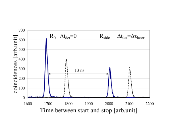
Figure 2: TAC histogram for two different ratios r. The straight line corresponds to $r$=2.5 (measured $\chi=0.95$) and the dotted line to $r$=0.2 (measured $\chi=0.3$) The two curves are artificially shifted for clarity.

Fig. 2 shows a typical TAC histogram for two different configurations (i.e. pump pulse duration and IF), leading to different values of $r$. For each value of $r$, one can directly measure the $\chi$ by comparing the number of coincidence counts $R_{0}$ in the central peak and $R_{side}$ in the side peak.

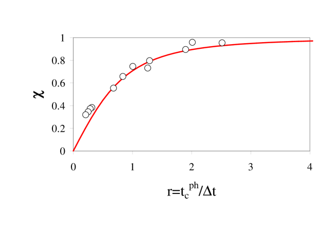
Figure 3: Measured $\chi$ coefficient as a function of the ratio $r$. The open circles are experimental points. The full line is a plot of formula (9).

Fig. 3 shows the measured $\chi$, as a function of the ratio $r$. The theoretical prediction described later is

$$\chi = \frac{r}{\sqrt{1+r^{2}}}\,,$$ (9)

which by the way reproduces the predictions of Section II in the limiting cases ($\chi=1$ for large $r$ and $\chi=r$ for small $r$). The agreement of the data with this prediction is satisfactory — note in particular that there are no free parameters in the model.

IV Theoretical description

IV.1 State after down-conversion

We want to describe the state of the e-m field produced as the output of a down-conversion process driven by a classical field. The scheme of the calculation is standard: the output state is

$$|\Psi\rangle = e^{-i{\cal{H}}}\mbox{$|0\rangle$}\,\simeq\,\big{(}\leavevmode\hbox{\small 1\normalsize\kern-3.30002pt1}-i{\cal{H}}-\frac{1}{2}{\cal{H}}^{2}\big{)}\mbox{$|0\rangle$}\,,$$ (10)

where ${\cal{H}}=\frac{1}{\hbar}\int H_{I}(t)dt$ and $H_{I}(t)$ is the Hamiltonian describing the down-conversion process in the interaction representation. This scheme has been applied in Refs. keller ; grice to the case in which the pump field is not a continuous cw wave but a pulse of finite spatio-temporal extension. In these Refs, the calculation was limited to the two-photon term. Wang et al. wang studied the four-photon term, for degenerate type-I down-conversion. Here we consider colinear emission (propagation along $z$) of non-degenerate photons in a type-I crystal.

The Fourier-transform of the pump field is written $\sqrt{I_{p}}\,\alpha(\omega)$. Following the same steps as in Refs. keller ; grice we find ${\cal{H}}\,=\,\sqrt{I}\,\left({\cal{A}}^{\dagger}\,+\,{\cal{A}}\right)$, where $I$ is proportional to the intensity $I_{p}$ of the pump field, and where ${\cal A}^{\dagger}$ is the two-photon creation operator

$${\cal A}^{\dagger} = \int d\omega_{1}\,d\omega_{2}\,\alpha(\omega_{1}+\omega_{2})\,\Phi(\omega_{1},\omega_{2})\,a^{\dagger}(\omega_{1})a^{\dagger}(\omega_{2})\,.$$ (11)

Here appears the phase-matching function $\Phi(\omega_{1},\omega_{2})$, peaked around $\omega_{1}\approx\Omega_{1}$ and $\omega_{2}\approx\Omega_{2}$ with $\Omega_{1}\neq\Omega_{2}$ phasematch . In the following for conciseness we shall write

$${\cal P}(\omega_{1},\omega_{2}) = \alpha(\omega_{1}+\omega_{2})\,\Phi(\omega_{1},\omega_{2})\,.$$ (12)

Now we must insert ${\cal{H}}$ into (10). Since ${\cal A}\mbox{$|0\rangle$}=0$ and ${\cal A}{\cal{A}}^{\dagger}\mbox{$|0\rangle$}\,\propto\,\mbox{$|0\rangle$}$, after removing the vacuum component that obviously does not contribute to the detection, one finds

$$|\Psi\rangle \simeq i\sqrt{I}\,{\cal A}^{\dagger}\mbox{$|0\rangle$}+\frac{I}{2}\,{{\cal A}^{\dagger}}^{2}\mbox{$|0\rangle$}\,.$$ (13)

IV.2 Probabilities and the observed $\chi$

From $|\Psi\rangle$ produced at the down-conversion, we can calculate the probabilities $P_{2}=I\mbox{$\langle 0|{\cal A}{\cal A}^{\dagger}|0\rangle$}$ and $P_{4}=\frac{I^{2}}{4}\mbox{$\langle 0|{\cal A}^{2}{{\cal A}^{\dagger}}^{2}|0\rangle$}$ of producing exactly two, respectively exactly four, photons. For this, one makes use of

$$\left[a(\omega),a^{\dagger}(\omega^{\prime})\right] = \leavevmode\hbox{\small 1\normalsize\kern-3.30002pt1}\,\delta(\omega-\omega^{\prime})\,$$ (14)

and of a corollary of this commutation rule, that reads

$$\langle 0|a(\omega^{\prime\prime})a(\omega^{\prime\prime\prime})a^{\dagger}(\omega)a^{\dagger}(\omega^{\prime})|0\rangle$$

$$=\delta(\omega-\omega^{\prime\prime})\delta(\omega^{\prime}-\omega^{\prime\prime\prime})$$

$$+\delta(\omega-\omega^{\prime\prime\prime})\delta(\omega^{\prime}-\omega^{\prime\prime})\,.$$ (15)

For $P_{2}$, the result is formally $P_{2}=I\int d\omega_{1}d\omega_{2}\left[|{\cal P}(\omega_{1},\omega_{2})|^{2}+{\cal P}(\omega_{1},\omega_{2}){\cal P}^{*}(\omega_{2},\omega_{1})\right]$. However, the second term of the sum is always zero because of the phase-matching condition (non-degenerate photons): in fact, the ranges of frequencies in which the first and the second argument of $\Phi$, and consequently of ${\cal P}$, lead to a non-zero contribution do not overlap. From now onwards, we simply consider that $\omega_{1}$ and $\omega_{2}$ are different, that is $\left[a(\omega_{1}),a^{\dagger}(\omega_{2})\right]=0$. Here is the point when our calculation differs from the one of Ref. wang . In conclusion, we have obtained

$$P_{2} = I\,\int d\omega_{1}d\omega_{2}|{\cal P}(\omega_{1},\omega_{2})|^{2}\,\equiv\,I\,J_{2}\,.$$ (16)

To calculate $P_{4}$, formula (15) is applied to the operators acting on both modes $a$ and $b$, and one obtains

$$P_{4} = \frac{1}{2}\,I^{2}\,\left[(J_{2})^{2}\,+\,J_{4}\right]$$ (17)

where, writing $d\underline{\omega}=d\omega_{1}d\omega_{b}d\omega_{1}^{\prime}d\omega_{2}^{\prime}$,

$$J_{4} \equiv \int d\underline{\omega}{\cal P}(\omega_{1},\omega_{2}){\cal P}(\omega_{1}^{\prime},\omega_{2}^{\prime}){\cal P}^{*}(\omega_{1}^{\prime},\omega_{2}){\cal P}^{*}(\omega_{1},\omega_{2}^{\prime})$$ (18)

$$= \int d\omega_{2}d\omega_{2}^{\prime}\,\left|\int d\omega_{1}{\cal P}^{*}(\omega_{1},\omega_{2}^{\prime}){\cal P}(\omega_{1},\omega_{2})\right|^{2}$$

One can verify that $0\leq J_{4}\leq(J_{2})^{2}$ wang . By comparison with eq. (1) we find $\chi_{0}\,\equiv\,J_{4}/(J_{2})^{2}$; here, the suffix ”0” means that this is the value of $\chi$ in the absence of any filtering after the SPDC.

Now we must move and describe our experiment. Two approaches are possible. The ”brute force” approach consists in effectively describing all the details of the experiment: write the pump pulse consisting of two well-separated pulses (this configuration gives similar experimental predictions as the one presented in section II, but is easier to compute), have mode $a$ evolve through the coupler, and finally compute the coincidence rate at the detectors. This calculation is lengthy, although not devoid of interest for the theorist; we give it as an Appendix. The second approach is more clever: we know that the experiment measures $\chi$ for a single pump pulse $g(\omega)$, in the presence of an interference filter. We can then apply all that we have just done to find immediately

$$\chi = J_{4}^{F}/\big{(}J_{2}^{F}\big{)}^{2}$$ (19)

where, writing $G(x,y)=g(x+y)\Phi(x,y)$ and $F(\omega)$ for the intensity profile of the filter, we have

$$J_{2}^{F} = \int d\omega_{1}d\omega_{2}F(\omega_{1})|G(\omega_{1},\omega_{2})|^{2}\,,$$ (20)

$$J_{4}^{F} = \int d\underline{\omega}\,F(\omega_{1})F(\omega_{1}^{\prime})\,G(\omega_{1},\omega_{2})G(\omega_{1}^{\prime},\omega_{2}^{\prime})G^{*}(\omega_{1}^{\prime},\omega_{2})G^{*}(\omega_{1},\omega_{2}^{\prime})\,.$$ (21)

Obviously, in the Appendix we obtain the same result.

IV.3 Explicit estimate

We have just found the general formulae that describe the quantity $\chi$ measured in our experiment. In this paragraph, we solve explicitly (20) and (21) using some crude approximations; the final result will be formula (9) for $\chi$, that has been shown to fit the experimental data.

We make the following hypotheses:
(i) The pump pulse is Fourier-transform limited: $g(\omega)=\left(2\pi\Delta_{p}\right)^{1/4}\,e^{-(\omega-\Omega_{p})^{2}/4\Delta_{p}^{2}}$.
(ii) The filter has a gaussian profile: $F(\omega)=\left(2\pi\Delta_{F}\right)^{1/2}\,e^{-(\omega-\Omega_{1})^{2}/2\Delta_{F}^{2}}$.
(iii) The coherence time of the photons is uniquely determined by the width of the filter: $t_{c}^{ph}=\Delta_{F}^{-1}$. Therefore we replace $\Phi(\omega_{1},\omega_{2})$ by 1, that is, $G(\omega_{1},\omega_{2})$ by $g(\omega_{1}+\omega_{2})$.

The big advantage of this set of hypotheses however is that we are left with two meaningful quantities: $\Delta_{p}$ and $\Delta_{F}$, whose inverses are the coherence times of the pump and of the photons in mode $a$. Plausible physical arguments will allow us to get rid of all these hypotheses at the end of the calculation.

The calculation of $J_{2}^{F}$ is straightforward: via the change of variables $(\omega_{1},\omega_{2})\rightarrow(\omega_{1},\xi=\omega_{1}+\omega_{2})$, the double integral factorizes into the product of two normalized gaussians, so $J_{2}^{F}=1$. This implies $\chi=J_{4}^{F}$. The calculation of this integral is longer but not difficult: by the usual technique of square completion, one first arranges the terms in order to integrate out $\omega_{2}$ and $\omega_{2}^{\prime}$; the result of this procedure, writing $\omega_{1}=x$ and $\omega_{1}^{\prime}=y$, is

$$J_{4}^{F}\,=\,\frac{1}{2\pi\Delta_{F}}\int dxdy\,\exp\left[-\frac{1}{2}\left(\frac{x^{2}+y^{2}}{\Gamma^{2}}-\frac{xy}{\Delta_{p}^{2}}\right)\right]$$ (22)

with $\frac{1}{\Gamma^{2}}=\frac{1}{\Delta_{F}^{2}}+\frac{1}{2\Delta_{p}^{2}}$. Using square completion again, one can integrate on $y$ first and on $x$ later. The result is $J_{4}^{F}=\frac{\Gamma}{\Delta}\,\frac{\Gamma^{\prime}}{\Delta}$ with $\frac{1}{\Gamma^{\prime 2}}\,=\,\frac{1}{\Gamma^{2}}-\frac{\Gamma^{2}}{4\Delta_{p}^{2}}$. A little more algebra leads to:

$$\chi\,=\,\frac{\tilde{r}}{\sqrt{1+\tilde{r}^{2}}}\,,\mbox{ with }\,\tilde{r}\,=\,\frac{\Delta_{p}}{\Delta_{F}}\,.$$ (23)

From this simple result, we guess the general result (9) by identifying $\tilde{r}$ with $r$. This step is motivated by the following considerations. One the one hand, since we took a Fourier-transformed limited pulse for the calculation, the coherence time of the pump $1/\Delta p$ is equal to the pulse duration, which we know to be the relevant quantity comment1 . On the other hand, $1/\Delta F$ is the coherence time of the down-converted photons, as long as the filter bandwidth is much smaller than the bandwidth of the unfiltered photons. When this condition is no longer satisfied, the relevant physical parameter is of course $t_{c}^{ph}$.

V Conclusion

We studied the physics of four-photon states in pulsed parametric down-conversion. The parameters of the experiment determine to which extent the four-photon state exhibits four-photon entanglement, or can be rather described as two independent pairs. Any intermediate situation is quantified by a single parameter $\chi$ that depends only on the ratio between the coherence time of the created photons and the duration of the pump pulse. A simple experiment to measure $\chi$ has been realized. A theoretical model based on the standard formalism of quantum optics has been derived, that fits well the experimental data. Beside its fundamental aspect, this work is of practical interest in quantum optics, because it provides a simple mean to quantify the ”coherence” of four photons states which is important for experiments such as quantum teleportation where independent photons must overlap at a beam splitter.
Note : For related independent works on the statistics of photon numbers in down-conversion, see stat

The authors would like to thank Claudio Barreiro and Jean-Daniel Gautier for technical support. Financial support by the Swiss NCCR Quantum Photonics, and by the European project RamboQ is acknowledged.

VI Appendix

In this appendix, we want to re-derive formulae (20) and (21) with a full calculation of the experiment sketched in Fig. 1.

For the experiment we are going to consider, the classical pump field will be composed by two identical pulses separated by a time $\tau$. This configuration leads to the same experimental results as the one presented before and is easier to compute. If $g(\omega)$ is the Fourier transform (FT) of each pulse, the FT of the pump field is then simply $\alpha(\omega)=g(\omega)(1+e^{i\omega\tau})$. To avoid multiplying notations, we keep ${\cal P}$ as in (12) for this explicit form of the pump field:

$${\cal P}(\omega,\tilde{\omega}) = (1+e^{i(\omega+\tilde{\omega})\tau})\,g(\omega+\tilde{\omega})\,\Phi(\omega,\tilde{\omega})\,$$ (24)

$$= \,(1+e^{i(\omega+\tilde{\omega})\tau})\,G(\omega,\tilde{\omega})\,.$$

VI.1 Evolution

As discussed, the photons are separated according to their frequency. Those whose frequency is close to $\Omega_{1}$ (resp. $\Omega_{2}$) are coupled into the spatial mode $a$ (resp. $b$). Photons in mode $b$ do not undergo any evolution, while mode $a$ evolves through a 50-50 coupler into modes $c=(a,+)$ and $d=(a,-)$ according to

$$a^{\dagger}(\omega) \longrightarrow \frac{c^{\dagger}(\omega)+i\,d^{\dagger}(\omega)}{\sqrt{2}}\,.$$ (25)

Inserting this evolution into (13), the state at the detection reads

$$\mbox{$|\Psi\rangle$}_{det} \simeq i\,{\cal K}\mbox{$|0\rangle$}+\frac{1}{2}\,{{\cal K}}^{2}\mbox{$|0\rangle$}$$ (26)

where, omitting the multiplicative constant $\sqrt{I/2}$, we have written

$${\cal K} = \int d\omega\,d\tilde{\omega}\,{\cal P}(\omega,\tilde{\omega})\,\left[c^{\dagger}(\omega)+id^{\dagger}(\omega)\right]\,b^{\dagger}(\tilde{\omega})\,.$$ (27)

VI.2 Detection (I): generalities

We turn now to the detection. The experiment that we are describing involves the detection of two-photon coincidences. Let $D_{c}$ and $D_{d}$ be the two detectors that monitor modes $c$ and $d$. The probability of detecting a coincidence between the two events ”photon detected in $D_{j}$ at the time $t_{j}$”, $j=c,d$, is given by

$$P_{D_{c},D_{d}}(t_{c},t_{d}) = ||E^{(+)}_{c}(t_{c})\,E^{(+)}_{d}(t_{d})\,\mbox{$|\Psi\rangle$}_{det}||^{2}$$ (28)

where

$$E^{(+)}_{c}(t_{c})\, = \,\int d\nu\,f_{c}(\nu)\,c(\nu)\,e^{-i\nu t_{c}}\,$$

$$E^{(+)}_{d}(t_{d})\, = \,\int d\nu\,f_{d}(\nu)\,d(\nu)\,e^{-i\nu t_{d}}$$ (29)

are the positive frequency component of the electric field at time $t_{j}$ in the mode detected by detector $D_{j}$ note0 , weighted by the amplitude of the filter $f_{j}(\nu)$ put in front of each detector. From now on, as in our experiment where the filter was actually put before the WDM, we consider $f_{c}=f_{d}=f$; the intensity shape of the filter is $F(\omega)=|f(\omega)|^{2}$.

Now we insert (26) into (28). As expected, the term linear in ${\cal K}$ gives no contribution: if there is just one photon in modes $c$ or $d$, no coincidence count can be obtained. Similarly, no contribution comes from the terms of the form $c^{\dagger}(\omega)c^{\dagger}(\omega^{\prime})$ and $d^{\dagger}(\omega)d^{\dagger}(\omega^{\prime})$ in ${\cal K}^{2}$, where both photons are found in the same mode after the coupler. In the calculation of the non-zero terms, we systematically omit multiplicative constants from now on. Using (14) for modes $c$ and $d$, one finds:

$$E^{(+)}_{c}(t_{c})\,E^{(+)}_{d}(t_{d})\,\mbox{$|\Psi\rangle$}_{det}=\int d\underline{\omega}\,e^{-i(\omega t_{c}+\omega^{\prime}t_{d})}\,\,f(\omega)\,f(\omega^{\prime}){\cal P}(\omega,\tilde{\omega}){\cal P}(\omega\,^{\prime},\tilde{\omega}\,^{\prime})\,b^{\dagger}(\tilde{\omega})b^{\dagger}(\tilde{\omega}\,^{\prime})\mbox{$|0\rangle$}\,,$$ (30)

where we have written $d\underline{\omega}=d\omega\,d\omega\,^{\prime}\,d\tilde{\omega}\,d\tilde{\omega}\,^{\prime}$. The probability $P_{D_{c},D_{d}}(t_{c},t_{d})$ is the square modulus of this expression. Using (15) for mode $b$, one finds

$$P_{D_{c},D_{d}}(t_{c},t_{d})=\int d\underline{\omega}\,e^{-i[(\omega-\hat{\omega})t_{c}+(\omega^{\prime}-\hat{\omega}^{\prime})t_{d})]}\,\big{[}K(\omega,\omega^{\prime},\hat{\omega},\hat{\omega}^{\prime};\tilde{\omega},\tilde{\omega}\,^{\prime})+K(\omega,\omega^{\prime},\hat{\omega}^{\prime},\hat{\omega};\tilde{\omega},\tilde{\omega}\,^{\prime})\big{]}$$ (31)

where we have written $d\underline{\omega}=d\omega\,d\omega\,^{\prime}\,d\hat{\omega}\,d\hat{\omega}\,^{\prime}\,d\tilde{\omega}\,d\tilde{\omega}\,^{\prime}$ and

$$K(\omega,\omega^{\prime},\hat{\omega},\hat{\omega}^{\prime};\tilde{\omega},\tilde{\omega}\,^{\prime}) = f(\omega)\,f(\omega^{\prime})\,f(\hat{\omega})\,f(\hat{\omega}^{\prime})\,{\cal P}(\omega,\tilde{\omega})\,{\cal P}(\omega\,^{\prime},\tilde{\omega}\,^{\prime}){\cal P}^{*}(\hat{\omega},\tilde{\omega})\,{\cal P}^{*}(\hat{\omega}^{\prime},\tilde{\omega}\,^{\prime})\,.$$ (32)

The detection rate (counts per pulse) is obtained by integrating $P_{D_{c},D_{d}}(t_{c},t_{d})$ over the time-resolution of the detector $2\Delta T$:

$$R(T_{c},T_{d}) = \int_{T_{c,d}\pm\Delta T}\,dt_{c}\,dt_{d}\,P_{D_{c},D_{d}}(t_{c},t_{d})\,.$$ (33)

The time-resolution must be longer than the coherence time of the photons (otherwise, the selected modes cannot be seen), and shorter than the spacing between the pulses, to allow the resolution in time-bins. As the result of this integration, $R(T_{c},T_{d})$ has the same form as $P_{D_{c},D_{d}}(t_{c},t_{d})$ given in (31), via the replacements

$$e^{-i(\omega-\hat{\omega})t_{c}} \rightarrow \Delta T\,e^{-i(\omega-\hat{\omega})T_{c}}\,\mbox{sinc}[(\omega-\hat{\omega})\Delta T]$$ (34)

$$e^{-i(\omega^{\prime}-\hat{\omega}^{\prime})t_{d}} \rightarrow \Delta T\,e^{-i(\omega^{\prime}-\hat{\omega}^{\prime})T_{d}}\,\mbox{sinc}[(\omega^{\prime}-\hat{\omega}^{\prime})\Delta T]\,.$$ (35)

Even if it seems redundant here, for subsequent ease, it is convenient to write down explicitly

$$R(T_{c},T_{d}) = R_{1}(T_{c},T_{d})+R_{2}(T_{c},T_{d})$$ (36)

where we have defined, writing $S(x)=\Delta T\mbox{sinc}(x\Delta T)$:

$$R_{1}(T_{c},T_{d}) = \int d\underline{\omega}\,e^{-i[(\omega-\hat{\omega})T_{c}+(\omega^{\prime}-\hat{\omega}^{\prime})T_{d})]}\,K(\omega,\omega^{\prime},\hat{\omega},\hat{\omega}^{\prime};\tilde{\omega},\tilde{\omega}\,^{\prime})\,S(\omega-\hat{\omega})S(\omega^{\prime}-\hat{\omega}^{\prime})\,,$$ (37)

$$R_{2}(T_{c},T_{d}) = \int d\underline{\omega}\,e^{-i[(\omega-\hat{\omega})T_{c}+(\omega^{\prime}-\hat{\omega}^{\prime})T_{d})]}\,K(\omega,\omega^{\prime},\hat{\omega}^{\prime},\hat{\omega};\tilde{\omega},\tilde{\omega}\,^{\prime})\,S(\omega-\hat{\omega})S(\omega^{\prime}-\hat{\omega}^{\prime})\,.$$ (38)

VI.3 Detection (II): meaningful times

We have just found an expression for $R(T_{c},T_{d})$. Now, recall that the first time-bin is defined by $T=0$, the second time-bin is defined by $T=\tau$. Therefore, we expect $R(T_{c},T_{d})$ to be significantly different than 0 only when $T_{c}$ and $T_{d}$ take the values $0$ or $\tau$. In particular, the counting rate in the central peak is $R_{c}=R(0,0)+R(\tau,\tau)$, while $R_{lat}=R(0,\tau)=R(\tau,0)$ are the counting rates in each of the lateral peaks. We want to recover all these results out of our general formula. In addition, we shall have manageable expressions for $R_{c}$ and $R_{lat}$, allowing a fit of the experimental data.

Let us start with a qualitative argument, that is enough for our purposes. Recall the expression (24) of ${\cal P}$. The spectral width of $g$ is larger than (equal to, for Fourier-transform limited pulses) $\frac{1}{\Delta t}$, which in turn is much larger than $\tau^{-1}$ since we want two well-separated pulses. This means that $g(\omega)$ is almost constant in a frequency range of width $\tau^{-1}$. The phase-matching function is also constant over such ranges, because its typical width is the inverse of the coherence time $t_{c}^{ph}$ of the down-converted photons. Now, suppose that $T_{c}$ and $T_{d}$ are $0$ or $\tau$. If one inserts (24) into the expression for $R(T_{c},T_{d})$ and develops the products, one finds that $R(T_{c},T_{d})$ is a sum of terms that are the product of $g$, $\Phi$ and a phase factor of the form $e^{i\Omega\tau}$, with $\Omega$ some algebric sum of the $\omega$’s. The arguments above prove that this phase fluctuates very rapidly in the frequency space, unless $\Omega\simeq 0$. Therefore, when we integrate over the $\omega$’s, all the terms will average to 0 but those whose phase factor is 1. Moreover, by direct check one can easily get convinced that if either of $T_{c}$ or $T_{d}$ is equal to a time when no photon is expected, say $\frac{\tau}{2}$ or $2\tau$, then no phases can be erased: the coincidence rate becomes zero. In summary, the first step to simplify $R(T_{c},T_{d})$ consists in writing down explicitly all the terms, and keep only those terms whose phase factor is 1. From now onwards, we admit that $T_{c}$ and $T_{d}$ are either $0$ or $\tau$.

Having erased terms that fluctuate as $\tau^{-1}$ in the frequency space, a further simplification is possible. The argument of the cardinal sine functions is $(\omega-\hat{\omega})\Delta T\sim\Delta T/t_{c}^{ph}$. But as we said, $\Delta T$ must be larger than $t_{c}^{ph}$, otherwise the photon cannot be seen by the detector. Therefore the cardinal sine will only be significant if $\omega\approx\hat{\omega}$, that is, we can replace $\mbox{sinc}[(\omega-\hat{\omega})\Delta T]$ with $\frac{1}{\Delta T}\,\delta(\omega-\hat{\omega})$.

All this simplification procedure is just a matter of patience. One finds that $R_{1}(0,0)=R_{1}(0,\tau)=R_{1}(\tau,0)=R_{1}(\tau,\tau)\equiv(J_{2}^{F})^{2}$ given in (20), while $R_{2}(0,0)=R_{2}(\tau,\tau)\equiv J_{4}^{F}$ given in (21), and $R_{2}(0,\tau)=R_{2}(\tau,0)=0$. In conclusion, the detection rates in the central peak and in each of the lateral peaks are:

$$R_{c} = R(0,0)+R(\tau,\tau)\,=\,2[(J_{2}^{F})^{2}+J_{4}]\,,$$ (39)

$$R_{lat} = R(0,\tau)\,=\,R(\tau,0)\,=\,(J_{2}^{F})^{2}\,,$$ (40)

and the ratio $R_{c}/2R_{lat}$ is equal to $1+\chi$ as announced.

References

- (1) L. Mandel, E. Wolf, Optical Coherence and Quantum Optics (Cambridge University Press, Cambridge, 1995), chap. 22.4
- (2) D.F. Walls, G.J. Milburn, Quantum Optics (Springer Verlag, Berlin, 1994), chap. 5.
- (3) W. Tittel, G. Weihs, Quant. Inf. Comp. 2, 3 (2001)
- (4) T.E. Keller, M.H. Rubin, Phys. Rev. A 56, 1534 (1997)
- (5) W.P. Grice, I.A. Walmsley, Phys. Rev. A 56, 1627 (1997)
- (6) G. Di Giuseppe et al., Phys. Rev. A 56, R21 (1997); W.P. Grice et al., Phys. Rev. A 57, R2289 (1998)
- (7) Z.Y. Ou, J.-K. Rhee, L.J. Wang, Phys. Rev. A 60, 593 (1999). The correspondence between the notations of this reference and ours is provided by and , whence .
- (8) H. Weinfurter, M. Zukowski, Phys. Rev. A 64, 010102 (2001)
- (9) J.C. Howell, A. Lamas-Linares and D.Bouwmeester, Phys. Rev. Lett. 88, 030401 (2002)
- (10) M. Eibl, S. Gaertner, M. Bourennane, C. Kurtsiefer, M. Zukowski, and H. Weinfurter, Phys. Rev. Lett 90, 200403 (2003)
- (11) H. de Riedmatten, I. Marcikic, W. Tittel, H. Zbinden and N. Gisin, Phys. Rev. A 67 022301 (2003)
- (12) I. Marcikic, H. de Riedmatten, W. Tittel, V. Scarani, H. Zbinden, and N. Gisin, , Phys. Rev. A 66, 062308 (2002)
- (13) In this context, it becomes clear why we said that the duration of the pump pulse and not its coherence time is important parameter. One could indeed imagine a pulse with whose coherence time is much shorter than (think for instance to a femto-second pulse that experienced chromatic dispersion). In this case, photons can be created in the whole duration of the pulse and consequently there are many temporal modes of the created photons inside the pump pulse, even if its coherence time is shorter than
- (14) M. Zukowski, A.Zeilinger and H. Weinfurter, Ann. NY Acad. Sci. 775, 91-102 (1995)
- (15) A. Lamas-Linares, J.C.Howell and D.Bouwmeester, Nature, 412 887-890 (2001)
- (16) In the limit , the intensity of each independent process must become very weak, since their sum must stay finite; so we must also consider , and the natural constraint is that the intensity times the number of processes should be the mean number of pairs: . In this limit, and . Moreover, . Thus we find and . It is well-known that the argument applies for all , because the Poisson distribution is the limit for the binomial distribution: W. Feller, An introduction to Probability Theory and its Applications (Wiley, New York, 1968), VI.5-6.
- (17) To find the factor , we start by where and are the standard deviation of the temporal and spectral intensities. The FWHM are then calculated with: .
- (18) We don’t need the explicit formula for this function in what follows; just note that, if we can neglect the -dependence of the term (that is, chromatic dispersion) and the -dependence of the non-linear susceptibility , the phase-matching function becomes equal to , see eq. (11) in grice for the exact definition of the functions and .
- (19) J. Peřina Jr, O. Haderka, M. Hamar, quant-ph/0310065; K. Tsujino, H. Hofmann, S. Takeuchi, K. Sasaki, submitted paper; presented by S. Takeuchi at the EQIS’03 conference, Kyoto, 4-6 September 2003
- (20) Here we write instead of , being the distance from the crystal to the detector. This amounts to a choice of the origin of time, which is irrelevant because experimentally we can synchronize at will the time-windows of the detectors. Moreover, we neglect the -dependence of the field amplitude, that we set to 1 because we don’t measure absolute intensities.