ACCELERATION OF QUANTUM ALGORITHMS USING THREE-QUBIT GATES

Abstract

Quantum-circuit optimization is essential for any practical realization of quantum computation, in order to beat decoherence. We present a scheme for implementing the final stage in the compilation of quantum circuits, i.e., for finding the actual physical realizations of the individual modules in the quantum-gate library. We find that numerical optimization can be efficiently utilized in order to generate the appropriate control-parameter sequences which produce the desired three-qubit modules within the Josephson charge-qubit model. Our work suggests ways in which one can in fact considerably reduce the number of gates required to implement a given quantum circuit, hence diminishing idle time and significantly accelerating the execution of quantum algorithms.

1 Introduction

The most celebrated and potentially useful quantum algorithms, which include Shor’s factorization algorithm[1] and Grover’s search[2], manifest the potential of a quantum computer compared to its classical counterparts.

Widely different physical systems have been proposed to be utilized as a quantum computer[3, 4]. The main drawback shared by most of the physical realizations is the short decoherence time. Decoherence[5] destroys the pure quantum state which is needed for the computation and, therefore, strongly limits the available execution time for quantum algorithms. This, combined with the current restricted technical possibilities to construct and control nanoscale structures, delays the utilization of quantum computation for reasonably extensive[6] algorithms.

The execution time of a quantum algorithm can be reduced by optimization. The methods similar to those common in classical computation[7] can be utilized in quantum compiling, constructing a quantum circuit[8] for the algorithm. Moreover, the physical implementation of each gate can and must be optimized in order to achieve gate sequences long enough, for example, to implement Shor’s algorithm within typical decoherence times[9].

Any quantum gate can be implemented by finding an elementary gate sequence [10, 11] which, in principle, exactly mimics the gate operation. In the most general case on the order of $4^{n}$ elementary gates are needed to implement an arbitrary $n$-qubit [12]. Fortunately, remarkably shorter polynomial gate sequences are known to implement many commonly used gates, such as the $n$-qubit quantum Fourier transform (QFT). In addition to the exact methods, quantum gates can be implemented using techniques which are approximative by nature [9, 13, 14, 15].

In this paper we consider the physical implementation of nontrivial three-gate operations. As an example of the power of the technique, we show how to find realizations for the Fredkin, Toffoli, and QFT gates through numerical optimization. These gates have been suggested to be utilized as basic building blocks for quantum circuits and would thus act as basic extensions of the standard universal set of elementary gates. However, the method presented can be employed to find the realization of any three-qubit gate. Having more computer resources available would allow one to construct gates acting on more than three qubits.

The numerical method allows us a straightforward and efficient way for finding the physical implementation of any quantum gate. Thus, the method may prove to be practical or even necessary for an efficient experimental realization of a quantum computer.

We concentrate on a hypothetical Josephson charge qubit register[16], since the experimental investigations of superconducting qubits is active; see, for instance, Refs. Pashkin - martinis. The scheme utilizes the number degree of freedom of the Cooper pairs in a superconducting Josephson-junction circuit. It is potentially scalable and it offers, in principle, full control over the quantum register. Moreover, the method employed here is easily extended to any physical realization providing time-dependent control over the physical parameters.

2 Physical Model

The physical implementation of a practical quantum algorithm requires that it is decomposed into modules whose physical realizations are explicitly known. In the quantum computer, the gate operations are realized through unitary operations $U$ that result from the temporal evolution of the physical state of the quantum register. The unitary evolution is governed by the Hamiltonian matrix, $H(\gamma)$, which describes the energy of the system for a given setting of physical parameters $\gamma$. In general, the parameters are time-dependent, $\gamma=\gamma(t)$. The induced unitary operator is obtained from the formal solution of the Schrödinger equation

$$U=\mathcal{T}\exp\left(-i\int_{\gamma(t)}H(\gamma(t))dt\right),$$ (1)

where $\mathcal{T}$ stands for the time-ordering operator and we have chosen $\hbar=1$.

We consider the Josephson charge qubit register as a realization of a quantum computer, see Fig. 1. The register is a homogenous array of mesoscopic superconducting islands and the states of the qubit correspond to either zero or one extra Cooper pair residing on the island. Each of the islands is capacitively coupled to an adjustable gate voltage, $V_{\rm g}^{i}(t)$. In addition, they are coupled to a superconducting lead through mesoscopic SQUIDs. We consider an ideal situation, where each Josephson junction in the SQUID devices has the same Josephson energy $E_{\rm J}$ and capacitance $C_{\rm J}$. The magnetic flux $\Phi_{i}(t)$ through the $i^{\rm th}$ SQUID loop is a control parameter which may be produced by adjustable current $I_{i}$. The qubit array is coupled in parallel with an inductor, $L$, which allows the interaction between the qubits.

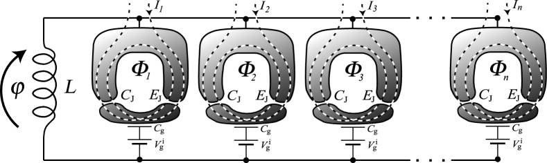
Figure 1: Schematic of an array of Josephson charge qubits coupled in parallel with an inductor.

In this scheme the Hamiltonian for the qubit register is[16, 9]

$$H=\sum_{i}^{n}\Bigl{\{}-\frac{1}{2}B^{i}_{z}\sigma_{z}^{i}-\frac{1}{2}B^{i}_{x}\sigma_{x}^{i}\Bigr{\}}-\sum_{i\neq j}^{n,n}CB^{i}_{x}B^{j}_{x}\sigma_{y}^{i}\otimes\sigma_{y}^{j},$$ (2)

where the standard notation for Pauli matrices has been utilized and $\sigma_{x}^{i}$ stands for $I\otimes\ldots\otimes\sigma_{x}\otimes I\ldots\otimes I$. Above, $B^{i}_{x}$ can be controlled with the help of a flux $\Phi_{i}(t)$ through the $i$th SQUID, $B^{i}_{z}$ is a tunable parameter which depends on the gate voltage $V_{\rm g}(t)$ and $C$ is a constant parameter describing the strength of the coupling. We set $C$ equal to unity by rescaling the Hamiltonian and time. The approach taken is to deal with the parameters $B^{i}_{z}$ and $B^{i}_{x}$ as dimensionless control parameters.

In the above Hamiltonian, each control parameter can be set to zero, to the degeneracy point, thereby eliminating all temporal evolution. The implementation of one-qubit operations is straightforward through the Baker-Campbell-Hausdorff formula, since the turning on of the parameters $B^{i}_{z}$ and $B^{i}_{x}$ one by one does not interfere with the states of the other qubits. Implementation of two-qubit operations is more complex since simultaneous application of nonzero parameter values for many qubits causes undesired interqubit couplings. However, by properly tuning the parameters it is possible to compensate the interference and to perform any temporal evolution in this model setup. This is partly why numerical methods are necessary for finding the required control-parameter sequences.

Finally, we point out that using the above Hamiltonian we are able to perform gates $U\in SU(2^{k})$ since the Hamiltonian is traceless. However, for every gate $U\in U(2^{k})$ we can find a matrix $U^{\prime}=e^{i\phi}U$ which has a unit determinant. The global phase factor $e^{i\phi}$ corresponds to redefining the zero level of energy.

3 Numerical Methods

We want to determine the physical realization for the quantum gates. Our aim is to numerically solve the inverse problem of finding the parameter sequences $\gamma(t)$ which would yield the desired gate operation when substituted into Eq. (1). The numerical optimization provides us with the realizations for not only any one- and two-qubit, but also for any three-qubit gates. Using the three-qubit implementation we circumvent the idle time in qubit control which provides us faster execution times, see Fig. 2.

In the Josephson charge qubit model the Hamiltonian for the $n$-qubit register, Eq. (2), depends on the external parameters $\gamma(t)=[B^{1}_{z}(t)\ldots B^{n}_{z}(t);\,B^{1}_{x}z(t)\ldots B^{n}_{x}(t)]$. To discretize the integration path $\gamma(t)$ for numerical optimization we consider a parametrization in which the values of the control-parameter fields, $\{B^{i}_{z}(t)\}$ and $\{B^{i}_{z}(t)\}$, are piecewise linear functions of time. Consequently, the path $\gamma(t)$ can be fully described by a set of parameter values at $\nu$ control points, where the slopes of the fields changes. We denote the set of these values collectively as $X_{\gamma}$. To obtain a general $k$-qubit gate $U_{k}\in SU(2^{k})$ one needs to have enough control parameters to parameterize the unitary group $SU(2^{k})$, which has a total of $2^{2k}-1$ generators. Since there are $2k$ free parameters for each control point in $\gamma$ we must have

$$2k\nu\geq 2^{2k}-1.$$ (3)

We use $\nu=12$ for the three-qubit gates and $\nu=4$ for the two-qubit gates. We force the parameter path to be a loop, which starts from and ends at the degeneracy point, where all parameter values vanish. Then we can assemble the modules in arbitrary order without introducing mismatch in the control parameters. We further set the time spent in traversing each interval of the control points to equal unity. Eventually, the execution time of $U_{k}$ is proportional to $\nu+1$, which gives us a measure to compare different implementations. Figure 2 illustrates our approach and shows the benefits of the three-qubit implementation of the Fredkin gate compared to corresponding implementation through two-qubit gate decomposition. Note that the two-qubit gate implementation could be further optimized[20].

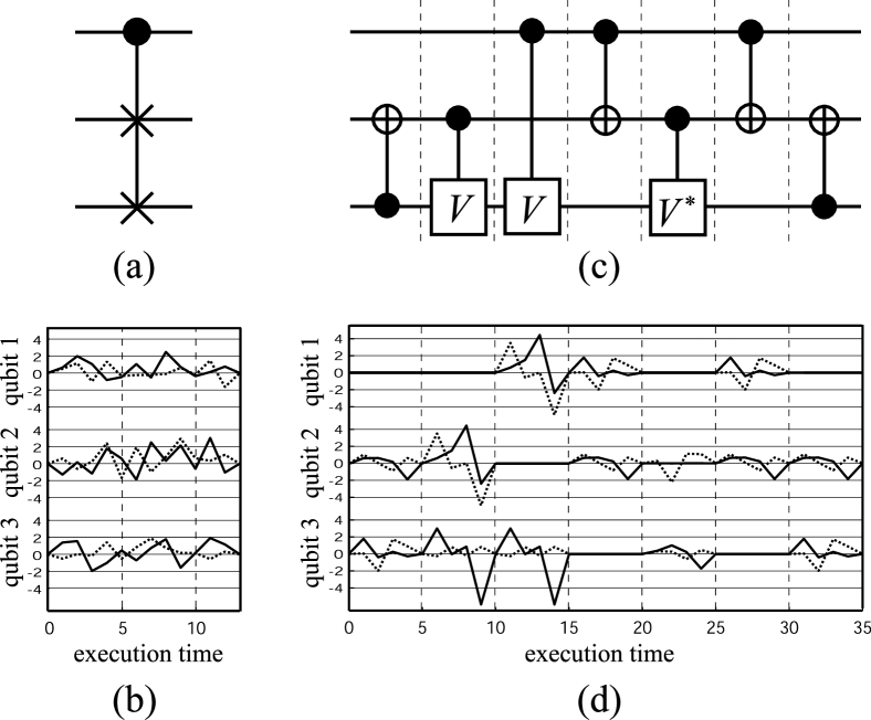
Figure 2: Implementation of the Fredkin gate on the Josephson charge qubit model. (a) The quantum circuit symbol of the Fredkin gate, and (b) its physical implementation by controlling all three qubits simultaneously. (c) The two-qubit gate decomposition of the Fredkin gate. Here $V=\sqrt{\sigma_{x}}$ and $V^{*}$ stands for its Hermitian conjugate. (d) The physical implementation of the gate sequence; note that during each gate operation, one of the qubits is in the idle state. The vertical axis in figures (b) and (d) stands for the control parameter field amplitudes; the solid line describes the parameter $B_{z}^{i}$ and the dotted line the parameter $B_{x}^{i}$, see text.

We evaluate the unitary operator in Eq. (1) in a numerically robust manner by dividing the loop $\gamma(t)$ into tiny intervals that take time $\Delta t$ to traverse. If $\gamma_{i}$ denotes all the values of the parameters in the midpoint of the $i^{th}$ interval, and $m$ is the number of such intervals, we then find to a good approximation

$$U_{X_{\gamma}}\approx\exp(-iH(\gamma_{m})\Delta t)\ldots\exp(-iH(\gamma_{1})\Delta t).$$ (4)

The evaluation of the $U_{X_{\gamma}}$ consists of independent matrix multiplications which can be evaluated simultaneously. This allows straightforward parallelization of the computation. To calculate the matrix exponentials efficiently we use the truncated Taylor-series expansion

$$e^{A}\approx\sum_{k=0}^{m}\frac{A^{k}}{k!},$$ (5)

where $m$ is an integer in the range $3$ – $6$. Since the eigenvalues of the anti-Hermitian matrix $A=-iH\delta t$ are significantly less than unity, the expansion converges rapidly. The applicability of the approximation can be confirmed by comparing the results with the exact results obtained using spectral decomposition.

Using the above numerical methods we transform the inverse problem of finding the desired unitary operator into an optimization task. Namely, any $\hat{U}$ can be found as the solution of the problem of minimizing the error function

$$f(X_{\gamma})=\|\hat{U}-U_{X_{\gamma}}\|_{F}$$ (6)

over all possible values of $X_{\gamma}$. Here $\|\cdot\|_{F}$ is the Frobenius trace norm defined as $\|{A}\|_{F}=\sqrt{\mathrm{Tr}\left({A}^{\dagger}{A}\right)}$. The minimization landscape is rough, see Fig. 3. Thus we apply the robust polytope search algorithm[21] for the minimization. We have assumed that a suitable limit of sufficient accuracy for the gate operations is given by the requirement of the applicability[6] of quantum error correction

$$\|U_{X_{\gamma}}-\hat{U}\|<10^{-4},$$ (7)

where $\hat{U}$ and $U_{X_{\gamma}}$ are the target and the numerically optimized gate operations, respectively.

Figure 3: Typical planar cut of the error function space. The plane through the minimum point $X_{\rm min}$ has been chosen arbitrarily in the parameter space. The irregular shape of the landscape easily reveals the complexity of finding the global minimum and the reason why the gradient-based methods fail.

4 Quantum Gate Optimization Results

We have applied the minimization procedure to various three-qubit gates and found that the error functional of Eq. (6) can be minimized to values below $10^{-4}$ by running the polytope search repetitively. Table 4 represents the optimized control parameters which serve to yield the Fredkin gate when applied to the Josephson charge qubit Hamiltonian. Numerical results for the Toffoli and three-qubit QFT gates are represented in Tables 4 and 4, respectively. Finding the control parameter using the polytope search requires on the order of $10^{6}$ error-function evaluations, which takes tens of hours of CPU time, but can be done in a reasonable time by using parallel computing.

We found that the error functional grows linearly in the vicinity of the minimum point $X_{\gamma}$, which implies that the parameter sequence found may be robust. The robustness was further analyzed by adding Gaussian noise to the control parameters of the path $\gamma(t)$. Such a sensitivity analysis confirmed that the error scales linearly with the root-mean-square amplitude of the surplus Gaussian noise.

Field amplitudes at the control points for the Fredkin gate. time $B_{z}^{1}$ $B_{z}^{2}$ $B_{z}^{3}$ $B_{x}^{1}$ $B_{x}^{2}$ $B_{x}^{3}$ 1 0.00000 0.00000 0.00000 0.00000 0.00000 0.00000 2 0.71637 -1.44846 1.54511 0.55428 0.67228 -0.58105 3 2.23337 0.18377 1.73522 1.29275 -0.69463 0.01513 4 1.17895 -1.31725 -2.22145 -1.11461 0.27210 -0.18665 5 -0.92555 1.97326 -1.15875 1.49438 2.69507 1.57872 6 -0.54804 0.66834 0.48872 -0.38981 -1.88659 -0.60226 7 1.18034 -2.13101 -0.81205 -0.27817 2.13894 0.92208 8 -0.59994 2.80989 0.82839 -0.24260 -1.09419 2.09561 9 2.78429 0.35914 1.98896 -0.11839 0.90439 0.83671 10 0.79364 2.40575 -1.78131 0.67600 3.31481 0.17828 11 -0.41098 -0.69585 0.15594 -0.21996 0.70917 0.15377 12 0.12630 3.39809 2.14043 1.65229 0.37794 -0.64223 13 0.84941 -1.17701 1.28801 -1.84075 1.16739 0.33965 14 0.00000 0.00000 0.00000 0.00000 0.00000 0.00000

Field amplitudes at the control points for the Toffoli gate. time $B_{z}^{1}$ $B_{z}^{2}$ $B_{z}^{3}$ $B_{x}^{1}$ $B_{x}^{2}$ $B_{x}^{3}$ 1 0.00000 0.00000 0.00000 0.00000 0.00000 0.00000 2 0.00286 -0.06484 0.96050 0.72386 0.33310 -0.22026 3 2.85647 -0.08874 2.94358 1.60795 -0.18192 0.03931 4 0.67879 -1.70364 -2.54280 -1.65771 -0.04722 -0.25411 5 -0.17379 0.87916 0.19581 1.55484 2.98447 1.22991 6 0.01847 2.68973 -0.18098 0.02898 -0.54301 -0.15977 7 0.21569 -3.27483 -0.33407 -0.31173 2.26503 0.32031 8 -0.57439 4.25644 1.25986 0.12262 0.06238 1.87619 9 3.40836 -0.48759 0.44296 -0.20867 0.04664 1.00381 10 -0.60520 1.59369 0.87620 0.95412 2.75968 0.37209 11 -0.10762 0.16258 -0.24672 -0.11839 1.38245 0.01990 12 0.20275 1.97553 1.12769 1.07003 0.46081 -0.35437 13 0.99088 -0.23145 0.68050 -2.12999 0.74237 0.01537 14 0.00000 0.00000 0.00000 0.00000 0.00000 0.00000

Field amplitudes for the three-qubit QFT gate. time $B_{z}^{1}$ $B_{z}^{2}$ $B_{z}^{3}$ $B_{x}^{1}$ $B_{x}^{2}$ $B_{x}^{3}$ 1 0.00000 0.00000 0.00000 0.00000 0.00000 0.00000 2 0.49824 0.41039 1.75837 0.42339 0.67345 1.83257 3 -0.18007 0.55372 -1.79297 0.64987 0.53048 -0.39300 4 0.73625 0.60488 -0.94171 0.61458 0.09641 -0.39863 5 2.21744 1.28419 2.82723 0.47046 1.04206 1.59345 6 0.47037 -0.48092 -0.53215 0.04297 0.21802 1.24063 7 0.69085 0.72558 1.00427 0.22332 1.25082 -0.25144 8 2.61154 0.87134 0.74335 0.31834 -0.00374 1.64643 9 0.24827 0.82952 1.04102 2.31043 1.00804 0.98377 10 -0.90785 -1.32491 1.10923 0.69935 -0.15359 -0.34420 11 0.59315 1.36082 -0.19764 1.83023 0.58541 0.85453 12 0.76819 0.31529 0.24531 -0.40221 1.13052 0.68184 13 -0.85651 0.02093 0.85491 1.33447 0.56580 0.06332 14 0.00000 0.00000 0.00000 0.00000 0.00000 0.00000

In our scheme, any three-qubit gate requires an integration path $\gamma(t)$ with 12 control points, which takes 13 units of time to execute. Similarly, a two-qubit gate takes 5 units of time to execute. Table 4 summarizes our results by comparing the number of steps that are required to carry out a single three-qubit gate or using a sequence of two-qubit gates. The results are calculated for the Fredkin and Toffoli gates following the decomposition given in Refs. Smolin and elementary. For a QFT gate the quantum circuit is explicitly shown, for example, in Ref. Gruska. Any three-qubit gate can be realized by using 68 controlled²$U$ and controlled² NOT gates. This number can be reduced to 50 using palindromic optimization[23]. The decomposition of the controlled²$U$ gate is discussed in Ref. elementary. Note that the results in Table 4 are calculated assuming that the physical realization for any two qubit modules is available through some scheme similar to the one which is employed in this paper and one-qubit gates are merged into two-qubit modules. The implementation of a general two-qubit module using a limited set of gates, for example, one-qubit rotations $R_{y}$ and $R_{z}$ and the CNOT gate has recently been discussed in Ref. Shende.

Comparison of the execution times for various quantum gates. gate Fredkin Toffoli QFT $U\in SU(2^{3})$ $U\in SU(2^{3})$ decomposed 3-qubit gates number of two-qubit gates 5 3 3 206 - execution time 25 15 15 1030 13

5 Discussion

We have shown how to obtain approximative control-parameter sequences for a Josephson charge-qubit register with the help of a numerical optimization scheme. The scheme utilizes well known theoretical methods and the results are obtained through heavy computation. Our method can prove useful for experimental realization of working quantum computers. The possibility to implement nontrivial multiqubit gates in an efficient way may well turn out to be a crucial improvement in making quantum computing realizable. For example, Josephson-junction qubits suffer from a short decoherence time, in spite of their potential scalability, and therefore the runtime of the algorithm must be minimized using all the possible ingenuity imaginable.

Here we have utilized piecewise linear parameter paths. This makes the scheme experimentally more viable than the pulse-gate solutions, since the parameters are adjusted such that no fields are switched instantaneously. However, the numerical method proposed for solving the time evolution operator is not unique. Some implicit methods for the integration in time may turn out to yield the results more accurately in the same computational time. Furthermore, for practical applications it may turn out to be useful to try and describe the parameter paths using a collection of smooth functions and to find whether they would produce the required gates.

To summarize the results of our numerical optimization, we emphasize that more efficient implementations for quantum algorithms can be found using numerically optimized three-qubit gates. In the construction of large-scale quantum algorithms even larger multiqubit modules may prove powerful. The general idea is to use classical computation to minimize quantum computation time, aiming below the decoherence limit.

References

- [1] P. W. Shor, in Algorithms for quantum computation: Discrete logarithms and factoring – Proc. 35nd Annual Symposium on Foundations of Computer Science, ed. S. Goldwasser, (IEEE Computer Society Press, 1994), p. 124.
- [2] L. K. Grover, Phys. Rev. Lett. 79, 325 (1997).
- [3] R. Clark (Ed.), Experimental Implementation of Quantum Computation (IQC ’01), (Rinton Press Inc., New Jersey, 2001).
- [4] F. De Martini (Ed.), Experimental Quantum Computation and Information (International School of Physics ”Enrico Fermi”, vol. 148) (IOS Press, Amsterdam, 2002).
- [5] W. H. Zurek, Rev. Mod. Phys. 75, 715 (2003).
- [6] D. P. DiVincenzo, Fortschr. Phys. 48, 771 (2000).
- [7] A. V. Aho, R. Sethi, and J. D. Ullman, Compilers: Principles, Techniques and Tools, (Addison-Wesley, Reading, Massachusetts, 1986).
- [8] D. Deutsch, Proc. R. Soc. London A 425, 73 (1989).
- [9] A. O. Niskanen, J. J. Vartiainen, and M. M. Salomaa, Phys. Rev. Lett. 90, 197901 (2003); J. J. Vartiainen, A. O. Niskanen, M. Nakahara, and M. M. Salomaa, “Implementing Shor’s algorithm on Josephson Charge Qubits”, quant-ph/0308171.
- [10] A. Barenco, C. H. Bennett, R. Cleve, D. P. DiVincenzo, N. Margolus, P. Shor, T. Sleator, J. Smolin, and H. Weinfurter, Phys. Rev. A 52, 3457 (1995).
- [11] J. Zhang, J. Vala, S. Sastry, and B. Whaley, Phys. Rev. Lett. 91, 027903 (2003).
- [12] V. V. Shende, I. L. Markov, and S. S. Bullock, “Minimal Universal Two-Qubit Quantum Circuits”, quant-ph/0308033.
- [13] A. W. Harrow, B. Recht, and I. L. Chuang, J. Math. Phys. 43, 4445 (2002).
- [14] E. Knill, “Approximation by quantum circuits”, quant-ph/9508006.
- [15] G. Burkard, D. Loss, D. P. DiVincenzo, and J. A. Smolin, Phys. Rev. B 60, 11404 (1999).
- [16] Y. Makhlin, G. Schön, and A. Shnirman, Rev. Mod. Phys. 73, 357 (2001).
- [17] Y. A. Pashkin, T. Yamamoto, O. Astafiev, Y. Nakamura, D. V. Averin, and J. S. Tsai, Nature 421, 823 (2003).
- [18] T. Yamamoto, Y. A. Pashkin, O. Astafiev, Y. Nakamura, D. V., and J. S. Tsai, Nature 425, 944 (2003).
- [19] J. M. Martinis, S. Nam, J. Aumentado, and C. Urbina, Phys. Rev. Lett. 89, 117901 (2002).
- [20] J. A. Smolin, and D. P. DiVincenzo, Phys. Rev. A 53, 2855 (1996).
- [21] J. C. Lagarias, J. A. Reeds, M. H. Wright, and P. E. Wright, SIAM J. Optim. 9, 112 (1998).
- [22] J. Gruska, Quantum Computing, McGraw-Hill, New York (1999), p. 118.
- [23] A. V. Aho and K. M. Svore, “Compiling Quantum Circuits using the Palindrome Transform”, quant-ph/0311008.