Stability of quantum Fourier transformation on Ising quantum computer

Abstract

We analyze the influence of errors on the implementation of the quantum Fourier transformation (QFT) on the Ising quantum computer (IQC). Two kinds of errors are studied: (i) due to spurious transitions caused by pulses and (ii) due to external perturbation. The scaling of errors with system parameters and number of qubits is explained. We use two different procedures to fight each of them. To suppress spurious transitions we use correcting pulses (generalized $2\pi k$ method) while to suppress errors due to external perturbation we use an improved QFT algorithm. As a result, the fidelity of quantum computation is increased by several orders of magnitude and is thus stable in a much wider range of physical parameters.

I Introduction

Quantum information theory Bennett is a rapidly evolving field. It uses quantum systems to process information and by doing so can achieve things that are not possible with classical resources. Quantum secure communication for instance is already commercially available. Quantum computation on the other hand is still far from being useful outside of the academic community. Two serious obstacles to overcome in building quantum computers are: (i) one must be able to control the evolution in order to precisely implement quantum gates, (ii) one must suppress all external influences. Errors in both cases are caused by the perturbation of an ideal quantum computer, either due to the internal imperfections in the first case or due to coupling with the “environment” in the second case. In the present paper we study both kind of errors in QFT algorithm and try to minimize them.

In order to be closer to the experimental situation we choose a concrete model of a quantum computer, namely the Ising quantum computer (IQC) Ising1st . IQC is one of the simplest models still having enough complexity to allow universal quantum computation. Quantum gates on this computer can be realized by the application of electromagnetic pulses. For the algorithm we choose to discuss QFT. The first reason to choose QFT is that it is one of the most useful quantum algorithms, giving exponential speedup over the best classical procedure known, and is also one of the ingredients of some other important algorithms, e.g. Shor’s factoring algorithm Shor . The second reason is that it is a complex algorithm, where by complex we mean it has more than ${\cal O}(n)$ number of quantum gates as opposed to previously studied more simple algorithms where the number of gates scales only linearly with the size of the computer (e.g. entanglement protocol DynFid ). Previous study of Shor’s algorithm in IQC IsingShor did not use recently introduced generalized $2\pi k$ method carlos which is the best known procedure for inducing transitions on IQC. It is easy to imagine that in most useful quantum algorithms the size of the program will grow faster than linearly with the number of qubits $n$ and therefore it is important to see how errors accumulate in such algorithms. This importance is confirmed by our results showing that errors due to unwanted transitions for QFT grow with the square of the number of pulses and not linearly as in algorithms with linear ${\cal O}(n)$ number of gates, for a typical state.

For QFT algorithm running on IQC we analyze errors due to spurious transitions caused by pulses, these we call intrinsic errors, and errors due to the coupling with an external “environment”, called external errors, modeled by a random hermitian matrix from a gaussian unitary ensemble (GUE) Guhr . We minimize intrinsic errors by applying some additional pulses to correct most probable errors carlos and by doing this, we are able to suppress intrinsic errors by several orders of magnitude. To suppress external errors due to GUE perturbation we use previously proposed improved quantum Fourier transformation (IQFT) IQFT which is more stable against GUE perturbations in a certain range of parameters. By using correlation function approach Corr we analyze in detail the dependence of errors on all relevant parameters and on the number of qubits $n$. By doing this we can set the limits between which parameters of IQC should lay in order to preserve the stability of computation. In our approach to decrease errors we do not use error correcting codes for the following reasons: we want to remove as many errors as we can on the lowest possible level and second, the intrinsic and external errors are not easily handled by error correcting codes (see Ref.Andrew and references therein).

The outline of the paper is as follows. In section II we repeat the definition of IQC and in section III we summarize linear response formalism which is the main theoretical tool for studying fidelity. In section IV we study intrinsic and external errors, first separately and then the case of both errors present at the same time. In the appendix we present the pulse sequences used to implement QFT and IQFT algorithms.

II Ising quantum computer

IQC consists of a 1-dimensional chain of $n$ equally spaced identical spin $1/2$ particles coupled by nearest neighbor Ising interaction of strength $J$, so that parallel spins are favored over anti-parallel ones by an energy difference of $J$ (we set $\hbar=1$ throughout the paper). The quantum computer is operated via an external magnetic field having two components. The first one is a permanent magnetic field oriented in the $z$ direction with a constant gradient which allows for the selective excitation of individual spins, while the second one is a sequence of $T$ circular polarized fields in the $x$-$y$ plane (which are called pulses) with different frequencies $\nu^{(m)}$, amplitudes (proportional to the Rabi frequencies $\Omega^{(m)}$), phases $\varphi^{(m)}$ and durations $\tau^{(m)}$ for the $m$th pulse, in which is encoded the protocol. A particular orientation of the register allows to suppress the dipole-dipole interaction between spins magicangle1 ; magicangle2 .

The Hamiltonian of the system is

$$\hat{H}=-\frac{1}{2}\sum_{l=0}^{n-1}\omega_{l}\hat{\sigma}_{l}^{z}-\frac{J}{2}\sum_{l=0}^{n-2}\hat{\sigma}_{l}^{z}\hat{\sigma}_{l+1}^{z}-\sum_{m=1}^{T}\hat{V}^{(m)}(t)\Theta^{(m)}(t)$$ (1)

with

$$\hat{V}^{(m)}(t)=\frac{\Omega^{(m)}}{4}\sum_{l=0}^{n-1}(\hat{\sigma}_{l}^{-}\exp\{-{\rm i}(\nu^{(m)}t+\varphi^{(m)})\}+\text{h.c.}),$$ (2)

$\Theta^{(m)}(t)$ equal to one during the $m$th pulse and zero otherwise, $\hat{\sigma}_{l}^{x,\,y,\,z}$ the usual Pauli operators for spin $l$ and $\hat{\sigma}_{l}^{\pm}=\hat{\sigma}_{l}^{x}\pm{\rm i}\hat{\sigma}_{l}^{y}$. Due to the constant gradient of the permanent magnetic field, the Larmor frequencies depend linearly on $l$, $\omega_{l}=(l+1)a$. By appropriately choosing the energy units we fix $J=1$ throughout the paper so that the only relevant energy scales are $\Omega^{(m)}$ and $a$. The basis states are chosen so that $\hat{\sigma}_{l}^{z}|0\rangle_{l}=|0\rangle_{l}$.

We will introduce the following notation for further discussion. Let the pulse $P_{i}^{ac}$ indicate a pulse with frequency $\nu_{i}^{ac}$ resonant with the flip of the $i$-th spin if its neighbors are in states “$a$” and “$c$”. This will induce the resonant transition $|\dots a_{i+1}b_{i}c_{i-1}\dots\rangle\to|\dots a_{i+1}\bar{b}_{i}c_{i-1}\dots\rangle$, named $T_{i}^{ac}$, if the pulse is a $\pi$ pulse ($a,b,c\in\{0,1\}$). Note that for edge qubits, i.e. $i\in\{0,n-1\}$, only one superscript is needed.

Operating IQC in the selective excitation regime, $\Omega^{(m)}\ll J\ll a$, allows one to separate transitions induced by pulses into three sets: resonant, near-resonant and non-resonant according to the detuning $\Delta$ of the transition which is the difference between the frequency of the pulse and the energy difference of the states involved in the transition. If $\Delta$ is exactly equal to zero, the transition is called resonant ($T_{i}^{ac}$ induced by the pulse $P_{i}^{ac}$), if $\Delta$ is of the order of $J$ it is called near-resonant ($T_{i}^{a^{\prime}c^{\prime}}$ induced by the pulse $P_{i}^{ac}$ with $\{a^{\prime},c^{\prime}\}\neq\{a,c\}$), and if $\Delta$ is of the order of $a$ it is called non-resonant ($T_{i^{\prime}}^{a^{\prime}c^{\prime}}$ induced by the pulse $P_{i}^{ac}$ with $i^{\prime}\neq i$). In the implementation of a protocol resonant transitions are the ones wanted, while near-resonant and non-resonant transitions are a source of error.

In the two level approximation magicangle1 , a given unwanted transition with detuning $\Delta$ is induced with probability

$$p=\frac{\Omega^{2}}{\Omega^{2}+\Delta^{2}}\sin^{2}{\left(\rho\frac{\pi}{2}\sqrt{1+\frac{\Delta^{2}}{\Omega^{2}}}\right)},$$ (3)

where $\rho$ is a dimensionless duration of the pulse (for a $\pi$ pulse $\rho=1$ and for $\pi/2$ pulse it is $1/2$). The most probable transitions are the near-resonant ones and these can be suppressed as briefly described in the next paragraph.

For $P_{i}^{10}(=P_{i}^{01})$ pulses all near-resonant transitions have the same detuning so setting $\Omega$ to $\Delta/\sqrt{4k^{2}-1}$ with $k$ an integer suppresses these transitions. Since for near-resonant transitions $\Delta={\cal O}(J)$, Rabi frequency is for all pulses of the order of $\Omega\approx J/k$. On the other hand, for $P_{i}^{00}$ and $P_{i}^{11}$ pulses near-resonant transitions have two different detunings therefore it is impossible to suppress both with a single pulse. This problem can be overcome adding an additional correcting $P_{i}^{10}$ pulse. The combination of these pulses in order to suppress all near-resonant transitions is called $Q$-pulse denoted by $Q^{ac}_{i\rho}$ when doing a $\rho\pi$ rotation of the $i\text{th}$ qubit if neighbors are in states “$a$” and “$c$”. This method to eliminate near-resonant transitions is called generalized $2\pi k$ method. We refer the interested reader to Ref. carlos for further details. $Q$-pulses are the basic building blocks of gates, which in turn are the building blocks of algorithms such as QFT and IQFT.

QFT for $n=4$ qubits can be written as

$$U_{\text{QFT}}={\text{T}}{\text{A}}_{0}{\text{B}}_{01}{\text{B}}_{02}{\text{B}}_{03}{\text{A}}_{1}{\text{B}}_{12}{\text{B}}_{13}{\text{A}}_{2}{\text{B}}_{23}{\text{A}}_{3}.$$ (4)

There are in total $n$ Hadamard A gates , $n(n-1)/2$ two-qubit B gates, ${\text{B}}_{jk}=\text{diag}\{1,1,1,\exp{({\rm i}\theta_{jk})}\}$, with $\theta_{jk}=\pi/2^{k-j}$ and one transposition gate T which reverses the order of qubits (e.g. ${\text{T}}|001\rangle=|100\rangle$). In total there are $n(n+1)/2+1$ gates. IQFT algorithm IQFT for $n=4$ qubits is given by

$$U_{\text{IQFT}} = \text{T}\text{A}_{0}\text{R}_{01}\text{R}_{02}\text{R}_{03}\text{G}_{01}\text{G}_{02}\text{G}_{03}$$ (5)

$$\times\text{A}_{1}\text{R}_{12}\text{R}_{13}\text{G}_{12}\text{G}_{13}\text{A}_{2}\text{R}_{23}\text{G}_{23}\text{A}_{3},$$

where ${\text{G}}_{ij}:={\text{R}}^{\dagger}_{ij}{\text{B}}_{ij}$. The R gate is defined by ${\text{R}}_{ij}|\dots a_{i}\dots b_{j}\dots\rangle:=(-1)^{b_{j}}|\dots a_{i}\dots(\overline{a_{i}}\oplus b_{j})\dots\rangle$. In total there are $n^{2}+1$ gates in IQFT, i.e. roughly two times as many as for QFT.

Recall that the implementation of quantum gates on IQC is easier in the interaction frame. Therefore, pulse sequences used in the paper implement the intended gates in the interaction frame. Each gate for QFT or IQFT (Eqs. (4) and (5)) must in turn be implemented by several pulses (see appendix). The number of pulses for QFT grows as $\sim 18n^{3}$ whereas it grows as $\sim 54n^{3}$ for IQFT. Note that this number can become very large, e.g. for IQFT and $n=10$ one has $44541$ pulses. Throughout the paper our basic unit of time will be either a gate (as written for instance in Eqs. (4) and (5)) or a pulse. A single exception will be the paragraph discussing correlation function of intrinsic errors, where the basic unit is a $Q$-pulse, which is composed of one or two pulses. The reason is that $Q$-pulses are the smallest near-resonant corrected unit of generalized $2\pi k$ method.

III Linear Response theory

As a criteria for stability we will use the fidelity $F(t)$, defined as an overlap between a state $\psi(t)$ obtained by an evolution with an ideal algorithm and the perturbed $\psi_{\delta}(t)$ obtained by the perturbed evolution:

$$F(t)=|\left\langle\psi_{\delta}(t)|\psi(t)\right\rangle|^{2},$$ (6)

where $|\psi(t)\rangle=U(t)|\psi(0)\rangle$ and $|\psi_{\delta}(t)\rangle=U_{\delta}(t)|\psi(0)\rangle$. To simplify matters we will assume time $t$ to be a discrete integer variable, denoting some basic time unit of an algorithm, like a gate or a pulse. The quantity measuring the success of the whole algorithm is the fidelity $F(t)$ at $t=T$ where $T$ denotes the number of gates (pulses). One of the most useful approaches to studying fidelity is using linear response formalism in terms of correlation function of the perturbation, for a review see Ref. Pregledni . This approach has several advantages. First it rewrites the complicated quantity fidelity in terms of a simpler one, namely the correlation function, simplifying the understanding of the fidelity. Second, the scaling of errors with the perturbation strength, Planck’s constant and with the number of qubits is easily deduced. Furthermore, as in practice one is usually interested in the regime of high fidelity, linear response is enough.

First we will shortly repeat linear response formulas as they will be useful for our discussion later. Let us write an ideal algorithm up to gate $t$ as $U(t)$

$$U(t)=U_{t}U_{t-1}\ldots U_{1},$$ (7)

where $U_{i}$ is the $i$-th gate (pulse). If $t=T$ we have a decomposition of a whole algorithm.

The perturbed algorithm can be similarly decomposed into gates

$$U^{\delta}(t)=U^{\delta}_{t}U^{\delta}_{t-1}\ldots U^{\delta}_{1}.$$ (8)

Each perturbed gate $U^{\delta}_{j}$ is now written as

$$U^{\delta}_{j}=\exp{(-{\rm i}\delta V_{j})}U_{j},$$ (9)

where $V_{j}$ is the perturbation of $j$-th gate and $\delta$ is a dimensionless perturbation strength. For any perturbed gate one can find a perturbation generator $V$, such that the relation (9) will hold. Observe that the distinction into perturbation strength $\delta$ and the perturbation generator $V$ in Eq. (9) is somehow arbitrary. If one is given an ideal gate $U$ and a perturbed one $U^{\delta}$ one is able to calculate only a product $\delta V$. This arbitrariness can always be fixed by demanding for instance that the second moment of the perturbation $V$ in a given state equals to $1$, $\langle V^{2}\rangle-\langle V\rangle^{2}=1$.

To the lowest order in the perturbation strength fidelity can be written as Corr

$$F(t)=1-\delta^{2}\sum_{t_{1},t_{2}=1}^{t}C(t_{1},t_{2}),$$ (10)

where the correlation function of the perturbation is

$$C(t_{1},t_{2})=\langle V_{t_{1}}(t_{1})V_{t_{2}}(t_{2})\rangle-\langle V_{t_{1}}(t_{1})\rangle\langle V_{t_{2}}(t_{2})\rangle$$ (11)

with $V_{j}(t)=U^{\dagger}(t)V_{j}U(t)$ being the perturbation of $j$-th gate propagated by an ideal algorithm up to time $t$, i.e. in the Heisenberg picture. The brackets $\langle\cdot\rangle$ denote the expectation value in the initial state. Throughout the paper we use random gaussian initial states and average over many of them to reduce statistical fluctuations. Note that the time dependence of the correlation function (11) is due to two reasons: one is time dependence due to the Heisenberg picture (time index in brackets) and the second one is due to the time dependence of the perturbation itself (time index as a subscript), i.e. one has different perturbations $V_{j}\neq V_{k}$ for different gates $j,k$. The expression for the fidelity Eq. (10) is the main result of the linear response theory of the fidelity. From this one can see that decreasing the correlation sum (or even making it zero, see Ref. Freeze ) will increase the fidelity. In Ref. IQFT stability of QFT algorithm was considered with respect to static GUE perturbation. Analyzing the correlation function they were able to design an improved QFT algorithm (IQFT) which increases fidelity.

We are mainly interested in the fidelity $F(T)$ at the end of an algorithm. The final time $T$ in useful quantum algorithms depends on the number of qubits in a polynomial way, say as $T\propto n^{p}$. The power $p$ depends on the algorithm considered and of course also on our decomposition of an algorithm into gates (pulses). For QFT and IQFT algorithms with decomposition into gates, Eqs. (4) and (5), one has $p=2$. On the other hand, for the implementation of QFT on IQC one needs $T\propto n^{3}$ ($p=3$) basic electromagnetic pulses, as one is not able to directly perform ${\text{B}}_{jk}$ gates on distant qubits but has to instead use a number of pulses proportional to the distance between the qubits $|j-k|$. Now if the correlation function decays sufficiently fast, the fidelity will decay like $F=1-\delta^{2}\sigma n^{p}$ whereas in the case of slow correlation decay the fidelity will decay as $F=1-\delta^{2}cn^{2p}$. In the extreme case of perturbations at different gates being statistically uncorrelated (very fast decay of correlations) $\langle V_{j}V_{k}\rangle\propto\delta_{jk}$ one obtains the exact formula $F=\exp{(-\delta^{2}n^{p})}$ IQFT . In the limit of large quantum computer (large $n$) strongly correlated static errors, giving slow decay of correlations, will therefore be dominant due to fast $\propto n^{2p}$ growth. When we will discuss errors caused by perturbations due to the coupling with the environment we will focus on static perturbations, meaning the same perturbation on all gates, $V_{k}=V_{j}=V$, as this component will dominate large $n$ behavior.

IV Errors in QFT

Errors in an experimental implementation of QFT algorithm on an IQC can be of three kinds: (i) due to unwanted transitions caused by electromagnetic pulses (ii) due to coupling with external degrees of freedom and (iii) due to variation of system parameters in the course of algorithm execution. In the present paper we will discuss only the first two errors. Errors due to electromagnetic pulses are inherent to all algorithms on an IQC as we are presently unable to design pulse sequences for quantum gates without generating some unwanted transitions albeit with small probabilities. This errors can be in principle decreased by going sufficiently deep into selective excitation regime but one must of course keep in mind the limitations of real experiments. Coupling with the “environmental” degrees of freedom is endemic in all implementations of quantum computers. As the environment will usually have many degrees of freedom we will model its influence on the quantum computer by some effective perturbation $V_{\text{eff}}$ given by a random matrix from a Gaussian unitary ensemble (GUE) Guhr . Note that coupling with the environment will generally cause non-unitary evolution of the central system. We expect quantum computation to be stable only on a time scale where evolution is approximately unitary, i.e. for times smaller than the non-unitarity time scale. Therefore we limit ourselves to unitary external perturbations. The third kind of errors due to the variation of system parameters, like e.g. variation of Larmor frequencies due to the variation of the magnetic field is not considered in this paper. This does not mean they are not important. Let us consider a systematic error in the gradient of the magnetic field throughout the protocol ($a\to a+\delta a$). Demanding that the error in the largest eigenphase at the end of the algorithm is much smaller than $1$, one gets the condition $a/\delta a\approx an^{p+2}/\Omega$. If one is in the selective excitation regime, this ratio can become very large and this puts a severe demand on the experiments.

To ease up understanding we will first discuss intrinsic errors only, then we will discuss external errors only and finally we will combine both errors.

IV.1 Intrinsic Errors

Let us consider probabilities of non and near-resonant transitions. For near-resonant and non-resonant transitions we have $\Delta\gg\Omega$ and the probability given by the perturbation theory is $p\propto(\Omega/\Delta)^{2}$. In the $2\pi k$ method Rabi frequency $\Omega$ is given as $\Omega\sim J/k$ so the probabilities for near-resonant and non-resonant transitions are

$$p^{\text{near}} \propto \left(\frac{1}{k}\right)^{2}$$

$$p^{\text{non}}_{jl} \propto \left(\frac{J}{ka(j-l)}\right)^{2},$$ (12)

where $p^{\text{non}}_{jl}$ denotes probability of a non-resonant transition with $\Delta\approx a|j-l|$ involving $j$-th and $l$-th spin, one of which is a resonant one. The dependence of near and non-resonant errors on system parameters is therefore different.

For pulse sequences used to generate QFT or IQFT we always used a generalized $2\pi k$ method by which one can get rid of all near-resonant transitions. Therefore the only errors that remain are non-resonant ones. We first checked numerically that this is indeed the case by studying dependence of errors on system parameters by which one is able to distinguish near and non-resonant errors, Eq. (12).

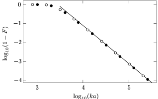
Figure 1: Dependence of fidelity on physical parameters of the system. Empty points indicate variation of $k$ with $a=100$, filled points indicate variation of $a$ with $k=128$, both for $n=6$. Full line is theoretical dependence of $p^{\text{non}}$ given by Eq. (12).

As one can observe from Fig. 1 the agreement with the theoretical $p^{\text{non}}$ (Eq. (12)) is excellent thereby confirming that the only errors left are non-resonant ones. By using generalized $2\pi k$ method we therefore decreased intrinsic errors by a factor of $(a/J)^{2}$ as compared to ordinary $2\pi k$ method where there are still some near-resonant errors present. In order to have complete understanding of fidelity decay due to intrinsic errors we have to understand scaling of these with the number of qubits. As we already discussed in section III this depends on two things: how strong the errors are correlated, giving possible scalings from $n^{p}$ to $n^{2p}$ and on the increase of the perturbation strength with the number of qubits. Let us first discuss the later. Under the assumption that the average transition probability (i.e. perturbation strength) for a non-resonant transition is the sum of all possible non-resonant transitions averaged over all possible resonant qubits, we can estimate

$$\delta\propto\frac{1}{n}\sum_{j\neq l=0}^{n-1}{p^{\text{non}}_{jl}}\ \ \underrightarrow{n\to\infty}\ \ \left[\frac{J}{ka}\right]^{2}\left(\frac{\pi^{2}}{3}-\alpha\frac{\log{n}}{n}\right),$$ (13)

with $\alpha$ some $n$ independent constant. We can see that the perturbation strength does not grow with $n$ asymptotically, but the convergence to its limit is logarithmically slow. For small $n$ the perturbation strength therefore will grow with $n$ whereas it will saturate for large $n$. The second contribution to the $n$-dependence of the fidelity comes from the dynamical correlations between errors given by the correlation function (11) of the perturbation generator for non-resonant errors. We numerically calculated this correlation function in order to understand how the correlation sum and therefore fidelity, Eq. (10), behaves as a function of $n$.

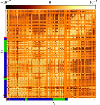
Figure 2: (Color online) Correlation function for intrinsic errors in QFT for $k=128$, $a=100$, $n=4$. The shading on time axes denotes the duration of different gates, Eq. (4), and the time going from $1$ to $543$ runs over all $Q$-pulses.

Figure 3: The correlation sum of the same data as in Fig. 2. Note the decrease of the sum when the transposition gate is applied. The fidelity is in this linear response regime simply given by Eq. (10). Vertical lines indicate beginning of each gate (Eq. (4)).

In Fig. 2 we show $C(t_{1},t_{2})$ averaged over all Hilbert space. One can see that there are large 2-dimensional regions of high correlations in all parts of the picture. This means there are strong correlations between errors at different pulses and therefore the correlation sum will likely grow as $\sim n^{6}$ as the number of pulses scales as $n^{3}$ for our implementation of QFT. Similar results are obtained also for IQFT as can be inferred from Fig. 4. One interesting thing to note is that during the application of the transposition gate at the end of the protocol the correlation sum starts to decrease at some point, nicely seen in Fig. 3 and also visible in the correlation picture in Fig. 2 as there are more negative than positive areas towards the end of the algorithm. This very interesting phenomena means that applying transposition at the end is advantageous (as compared to doing it classically for instance) as it will decrease non-resonant errors. We checked that this principle can not be exploited further by repeating transposition many times and by this decreasing correlation sum even more. Still, this surprising behavior suggests that it might be possible to decrease non-resonant errors in a systematic way.

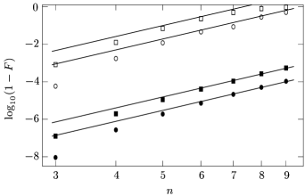
Figure 4: Dependence of fidelity on the number of qubits. Empty symbols indicate data for $k=128$ and $a=100$ while filled symbols are for $k=1028$ and $a=1000$. Circles indicate QFT and squares IQFT. In the presence of only intrinsic errors, IQFT does not improve fidelity. Full lines show asymptotic $n^{6}$ dependence.

To furthermore confirm predicted $\sim n^{6}$ growth of the correlation sum we calculated the dependence of intrinsic errors on $n$. This can be seen in Fig. 4, where we plot $1-F(T)$ as a function of $n$ for QFT and IQFT and for two different sets of parameters, one for $k=128$, $a=100$ giving large errors and one for $k=1024$, $a=1000$. One can see that asymptotically for large $n$ the dependence is indeed $n^{6}$ but the convergence to this behavior is fairly slow, one needs of the order of $n=7$ or more qubits. This slow convergence we believe is due to the logarithmic convergence of the perturbation strength (Eq. (13)). To get exact coefficients in front of $n^{6}$ dependence we fitted dependences of errors in Fig. 4 with a polynomial in $n$ using at most two nonzero terms. Defining polynomials in the linear response regime as $s^{\text{in}}=(1-F)(ka/J)^{2}$ one gets for QFT and IQFT

$$s^{\text{in}}_{\text{QFT}}(n) = 280n^{6}-660n^{5}$$

$$s^{\text{in}}_{\text{IQFT}}(n) = 1300n^{6}-2100n^{5}.$$ (14)

Both expressions are good for $n\geq 5$ and superscript “in” denotes intrinsic errors. Beyond the linear response the exponential dependence is frequently justified Corr and one has

$$F=\exp{\left(-\left[\frac{J}{ka}\right]^{2}s^{\text{in}}(n)\right)}.$$ (15)

Large coefficients of polynomials in Eqs. (14) are due to large number of pulses. The maximum possible dependence in the case of no decay of correlation function (see discussion at the end of section III) could be $T^{2}$ and therefore the leading terms in polynomials (14) expressed by the number of pulses are $s^{\text{in}}_{\text{QFT}}\sim 0.8T_{\text{QFT}}^{2}$ and $s^{\text{in}}_{\text{IQFT}}\sim 0.5T_{\text{IQFT}}^{2}$. Therefore relative to the number of pulses IQFT slightly decreases non-resonant errors but in the absolute sense QFT is better simply because it has only one third as many pulses as IQFT and the coefficient in front of $n^{6}$ (Eq. (14)) is thereby smaller. If only intrinsic errors in the generalized $2\pi k$ method are concerned QFT is always more stable than IQFT. Note that the intrinsic errors due to non-resonant transitions for QFT grow as $\sim T^{2}$ ($\sim n^{6}$) whereas in previously studied “simple” algorithms, for instance entanglement protocol DynFid , they grow only as the first power of the number of gates $\sim T$. This means that QFT is much more sensitive to intrinsic errors.

IV.2 External Errors

In order to study only external errors we set throughout this section parameters to $k=1024$ and $a=1000$, for which intrinsic errors are much smaller than external ones.

External error will be modeled by the perturbation $V$ (Eq. (9)) chosen to be a random hermitian matrix from a GUE ensemble. To facilitate comparison with previous results on IQFT IQFT we will make perturbation after each quantum gate, except for the last transposition gate T, Eq. (4), after which we do not make perturbation. So for QFT we make $n(n+1)/2$ perturbations, while for IQFT we make $n^{2}$ perturbations. One other possible choice would be to make perturbations after each pulse. We will discuss this possibility at the end of this section. For now let us just say that qualitatively the results are the same as if doing perturbation after each gate, one just has to rescale perturbation strength like $\delta_{\text{gate}}\propto n\delta_{\text{pulse}}$ as there are effectively ${\cal O}(n)$ perturbations (pulses) per gate.

The implementation of QFT on IQC is written in the interaction picture. As the static perturbation is the worst, meaning it will asymptotically in large $n$ limit be dominant, we will concentrate only on static perturbation, i.e. the same perturbation for all gates (pulses) $V_{j}=V_{k}=V$. There are still two possibilities, either making static perturbation in the interaction frame or making it static in the laboratory frame. Let us first discuss the later case. If we make static perturbation in the laboratory frame, we can of course transform it to the interaction frame by a unitary transformation $W(t)=\exp(-{\rm i}H_{0}t)$ given by the time independent part $H_{0}$ of the Hamiltonian Eq. (1). This transformation

$$\exp{(-{\rm i}\delta V_{\text{int}}(t))}:=W^{\dagger}(t)\exp{(-{\rm i}\delta V_{\text{lab}})}W(t),$$ (16)

will result in the perturbation in the interaction frame $V_{\text{int}}(t)$ being time dependent. As the transformation to the laboratory frame $W(t)$ in the selective excitation regime involves large phases, perturbations at different gates will tend to be uncorrelated due to averaging out of widely oscillating factors in the correlation function (11). Therefore in the first approximation one can assume $C(t_{1},t_{2})=\delta_{t_{1},t_{2}}$ and the fidelity will in this extreme case of uncorrelated errors decay as $F(T)=\exp{(-\delta^{2}T)}$ IQFT . On the other hand, if we make perturbation to be static in the interaction frame and the correlation function is not Kronecker delta in time, the fidelity will decay faster with the number of qubits (or $T$). To numerically confirm these arguments, we show in Fig. 5 dependence of fidelity with the number of qubits $n$ for the two cases discussed, static perturbation in the interaction frame and static perturbation in the laboratory frame. Polynomial fitting of $n$ dependence for QFT gives

$$s^{\text{gue}}_{\text{lab}}(n) = 0.47n^{2}+1.41n-2.42$$

$$s^{\text{gue}}_{\text{int}}(n) = 0.45n^{3}-0.42n^{2}+0.58n.$$ (17)

The fidelity due to external GUE errors is given as

$$F=\exp{(-\delta^{2}s^{\text{gue}}(n))},$$ (18)

with the appropriate $s^{\text{gue}}(n)$ from Eq. (17). Note that $s^{\text{gue}}_{\text{int}}(n)$ grows faster than $s^{\text{gue}}_{\text{lab}}(n)$ as argued. Observe also that for the static perturbation in the laboratory frame using the assumption of uncorrelated errors in the interaction frame we predicted $s^{\text{gue}}_{\text{lab}}\approx T\approx n^{2}/2$ for QFT which is remarkably close to the numerically observed value Eq. (17). For IQFT and the application of GUE perturbation in the laboratory frame one gets a similar result with the leading term $s^{\text{gue}}_{\text{lab}}(n)\sim 1.12n^{2}$. One can write an arbitrary time dependent perturbation in the interaction frame as a Fourier series and for large $n$ the static component will always prevail. Therefore, from now on we will exclusively discuss only static perturbations in the interaction frame.

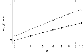
Figure 5: Dependence of $1-F$ in QFT algorithm on the number of qubits for static perturbation in the interaction frame (empty points) and in the laboratory frame (full points), with $\delta=0.04$. Lines are best fitting polynomials (see Eq. (17)).

The dependence of errors due to GUE perturbation in the case of QFT and IQFT has already been derived . For IQFT numerical fitting in our case gives dependence

$$s^{\text{gue}}_{\text{IQFT}}(n)=1.31n^{2}+0.86n-3.73.$$ (19)

Here the perturbation is again static in the interaction frame as is the case throughout the paper with a single exception being the previous paragraph. Dependence of fidelity in both cases for QFT and IQFT can be seen in Fig. 6, together with the theory (Eq. (18)) using polynomials (19) and (17).

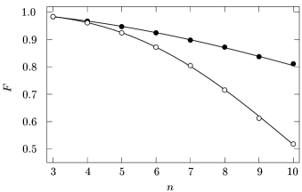
Figure 6: Dependence of fidelity on the number of qubits for QFT (empty symbols) and IQFT (filled symbols) algorithms ($\delta=0.04$). Curves are theoretical prediction Eq. (18) using polynomials from Eqs. (19) and (17).

Observe that IQFT for $n>n_{\text{crit}}=3$ is better than QFT despite having more gates and therefore applying perturbation on it more times (for $n\leq 3$ QFT is slightly better). What is important is that the dependence of errors on $n$ is also different, $\sim n^{3}$ for QFT, but only $\sim n^{2}$ for IQFT. This means that asymptotically IQFT is much more stable against GUE perturbations than ordinary QFT.

Finally, let us discuss what happens if we make static GUE perturbations in the interaction frame after each pulse, and not after each gate as done so far. The product of two operators $\exp{(-{\rm i}\delta V)}U$ can be written as $\exp{(-{\rm i}\delta V)}U=U\exp{(-{\rm i}\delta V(1))}$, with $V(1):=U^{\dagger}VU$. Using this expression for all errors within a single gate and bringing them all to the beginning of the gate we get

$$\exp{(-{\rm i}\delta V)}U_{r}\cdots\exp{(-{\rm i}\delta V)}U_{1}\approx$$

$$U_{r}\cdots U_{1}\exp{(-{\rm i}\delta[V(1)+\cdots+V(r)])},$$ (20)

where $r$ is number of pulses constituting a gate. This means that the application of the perturbation after each pulse is to the lowest order in $\delta$ equivalent to the application of the effective perturbation $\delta\sum_{j}^{r}{V(j)}$ after the gate. Of course now the perturbation is explicitly time dependent. But for a GUE matrix acting on a whole Hilbert space individual pulses will do transformations on an exponentially small subspace (i.e. on one qubit) and therefore one might expect that effectively one can write $\delta\sum_{j}^{r}{V(j)}\approx rV_{\text{eff}}$, where $V_{\text{eff}}$ is some effective random matrix independent of the gate. As in our case of QFT on IQC we have on average $\propto n$ pulses for a single gate we can predict that doing perturbation with strength $\delta_{\text{pulse}}$ after each pulse is approximately equal as doing perturbation of strength $\delta_{\text{gate}}\approx n\delta_{\text{pulse}}$ after each gate. In order to confirm these expectations we did numerical experiments with the results shown in Fig. 7.

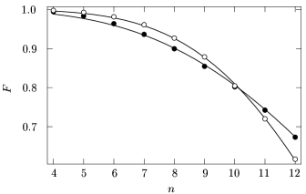
Figure 7: Dependence of $F$ on the number of qubits for the static GUE perturbation after each pulse with $\delta=5\cdot 10^{-4}$. Empty symbols are for QFT and filled symbols are for IQFT. Curves are theoretical prediction Eq. (18) using best fitting polynomials given by Eq. (21).

Fitting polynomial in the dependence of fidelity, Eq. (18), for QFT and IQFT gives in this case

$$s^{\text{gue}}_{\text{QFT}}(n) = 4.86n^{5}+35.8n^{4}$$

$$s^{\text{gue}}_{\text{IQFT}}(n) = 25.6n^{4}+606n^{3}.$$ (21)

The leading dependence of $n^{5}$ for QFT and $n^{4}$ for IQFT nicely agrees with our rescaling prediction $\delta_{\text{gate}}\approx n\delta_{\text{pulse}}$. IQFT is asymptotically again better than QFT as the errors grow slower with the number of qubits. The crossing point between the two in this case happens at $n_{\text{crit}}=10$, whereas in the case of perturbation after each gate we had $n_{\text{crit}}=3$. This confirms that doing GUE perturbation after each pulse is qualitatively the same as doing it after each gate, only the crossing point between QFT and IQFT changes and of course also the dependence of errors on $n$ changes, simply due to the different number of applied perturbations. If perturbation strength $\delta$ is properly rescaled, the $n$ dependence is the same in both cases.

Up to now we discussed intrinsic errors and external errors separately. The next question is of course, what happens if both errors are present at the same time and are of similar strength?

IV.3 Intrinsic and External Errors combined

If both kinds of errors are present, a first naive guess would be that they just add,

$$F^{\text{both}}=F^{\text{in}}F^{\text{gue}}=\exp{\left(-\left[\frac{J}{ka}\right]^{2}s^{\text{in}}(n)-\delta^{2}s^{\text{gue}}(n)\right)},$$ (22)

with the appropriate polynomials $s^{\text{in}}(n)$ and $s^{\text{gue}}(n)$ given in previous Eqs. (14), (17) and (19). In the linear response regime this formula means that both errors are uncorrelated, i.e. their cross-correlations are zero. This is easy to proof using properties of GUE matrices. Let us calculate cross-correlation function between $V^{\text{in}}(t_{1})$ and $V^{\text{gue}}(t_{2})$ averaged over GUE ensemble. Written explicitly one has to average products of the form $V^{\text{in}}_{ij}V^{\text{gue}}_{jk}$, where $V^{\text{gue}}$ is a GUE matrix. As this expression is linear in $V^{\text{gue}}$ it averages to zero, $\langle V^{\text{in}}_{ij}V^{\text{gue}}_{jk}\rangle_{\text{gue}}=0$, thereby explicitly confirming a simple additions of both errors. Of course in real experiments we are not averaging over GUE ensemble but are taking one definite representative member of it. But for large Hilbert space the expectation value of a typical random state and one particular GUE matrix is “self-averaging” and will be equal to the ensemble average.

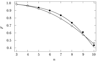
Figure 8: Fidelity for QFT (empty symbols) and IQFT (filled symbols) algorithm and GUE perturbation after each gate. System parameters are $k=a=200$ and $\delta=0.04$ (intrinsic and external errors are comparable in size). Full curves are theoretical predictions for $F$ given by Eq. (22).

Let us check the theoretical prediction for fidelity Eq. (22) with a numerical experiment. We again apply GUE perturbation after each gate. The results together with the theoretical prediction Eq. (22) are in Fig. 8. The agreement between the theory and the experiment is good also beyond the linear response regime. Please note that we deliberately choose parameters so that both QFT and IQFT give similar fidelity in order to also see the crossing of the two curves within the shown range of $n$. Given fixed $\delta$ and $ka$, QFT is always better for large $n$ because intrinsic errors will prevail over external ones, due to their fast $n^{6}$ growth. But still, for intermediate $n$’s IQFT can be better that QFT as seen in Fig. 8.

Now we are equipped with understanding of errors in QFT and IQFT due to external GUE perturbation and intrinsic errors so we can make some predictions regarding ranges of experimental parameters $ka$, $\delta$, $n$ for which the fidelity will be high enough. Interesting question for instance is, when is IQFT better than QFT? To find that, we set $F_{\text{QFT}}=F_{\text{IQFT}}$ with $F$’s given by Eq. (22). This results in the condition

$$\delta_{\text{crit}}=\frac{J}{ka}\sqrt{\frac{s^{\text{in}}_{\text{QFT}}-s^{\text{in}}_{\text{IQFT}}}{s^{\text{gue}}_{\text{QFT}}-s^{\text{gue}}_{\text{IQFT}}}}.$$ (23)

For $\delta>\delta_{\text{crit}}$ IQFT is better than QFT.

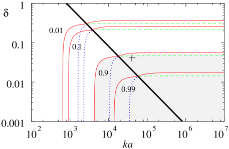
Figure 9: (Color online) Dependence of fidelity on system parameter $ka$ and GUE perturbation strength $\delta$ for $n=5$. Full curves of constant fidelity are composed of two parts corresponding to QFT or IQFT. Above the thick line for $\delta_{\text{crit}}$ IQFT is better and below QFT is better. Dotted curves of constant fidelity below this line are for IQFT and dashed lines above are for QFT. The shaded region corresponds to the region of fidelity larger than $0.9$. The plus symbol shows the position of parameters for Fig. 8.

In Fig. 9 we show curves of constant fidelity for $n=5$. They are composed of two parts, above the line for $\delta_{\text{crit}}$ IQFT is better than QFT, and below vice versa. Two characteristic features are also vertical and horizontal asymptotes of the curves of constant fidelity. The vertical asymptote means that for fixed $n$, even if $\delta=0$, we must have $ka$ larger than some critical value determined just by intrinsic errors, in order to have given fidelity. Horizontal asymptote for high $ka$ means that if $\delta$ is larger than some critical value, increasing $ka$ will not help to improve fidelity.

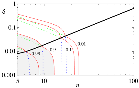
Figure 10: (Color online) Fidelity dependence on $\delta$ and number of qubits $n$ for a fixed value of $ka=10^{5}$. For the explanation of various curves see the caption to Fig. 9.

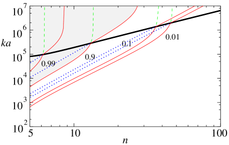
Figure 11: (Color online) Fidelity dependence on $ka$ and $n$ for a fixed $\delta=0.01$. For the explanation of various curves see the caption to Fig. 9.

In Figs. 10 and 11 we show similar plots, only these time one of the axes is dependence on $n$. For instance, from Fig. 10 on can see that having $ka=10^{5}$, the maximum number of qubits is $n\approx 12$ if we want to have fidelity larger than $0.9$ (even if $\delta=0$). This unfavorable growth of required $ka\propto n^{3}$ in order to have a fixed fidelity is due to $\sim n^{6}$ growth of intrinsic errors. It would therefore be advantageous to find a way to suppress errors due to non-resonant transitions kamenev .

V Conclusions

We analyzed two possible errors in the implementation of QFT on IQC working in the selective excitation regime. We consider: (i) intrinsic errors due to unwanted transitions caused by pulses, (ii) external errors due to coupling with the external degrees of freedom. We carefully analyze their dependence on system parameters and on the number of qubits. To diminish intrinsic errors we use the generalized $2\pi k$ method by which we are able to suppress all near-resonant transitions, with only much smaller non-resonant transitions remaining. We then study these non-resonant errors in QFT algorithm and by using correlation function formalism explain their growth with time as $\sim T^{2}$, in contrast to so far studied “simple” algorithms (having ${\cal O}(n)$ gates), where the growth is linear in time. The immediate question is whether this behavior is general for algorithms having more than ${\cal O}(n)$ gates. This very fast growth with $n$ is a consequence of strong correlations between errors at different pulses and puts a severe demand on experimental requirements. Therefore it would certainly be desirable to find a way to suppress also non-resonant errors. We also consider perturbations due to coupling with external degrees of freedom modeled by a random GUE matrix. To suppress this kind of errors we show that it is advantageous to use an improved QFT algorithm, for which the errors grow only as $\sim n^{2}$, whereas they grow as $\sim n^{3}$ for ordinary QFT. By a combination of both techniques, the generalized $2\pi k$ method and improved QFT algorithm, we are able to make implementation of QFT stable in a much wider range of parameters.

*

Appendix A QFT and IQFT implementation on the Ising Quantum Computer

To implement the protocol with high fidelity we use $Q_{i\rho}^{ab}$ pulses derived in Ref. carlos , which completely suppress all near-resonant errors. Phases of $Q$-pulses composing a gate must be chosen correctly so that the gate works on an arbitrary state. The protocols implementing $\text{CN}_{ij}$ (control not gate) and $\text{N}_{j}$ (not gate) can be found in sections 7.1-7.3 of Ref. carlos .

In order to complete QFT and IQFT we still need to implement the $\text{R}^{\dagger}$, R, A, B and T gates. We can decompose R, $\text{R}^{\dagger}$ and T gates into simpler pieces:

$$\text{R}_{ij} = \text{N}_{i}\text{CN}_{ij}\text{N}_{i}\text{Z}_{j},$$ (24)

$$\text{R}_{ij}^{\dagger} = \text{N}_{i}\text{Z}_{j}\text{CN}_{ij}\text{N}_{i},\text{ and}$$ (25)

T $$= \prod_{i=1}^{q}\prod_{j=1}^{q-i}\text{S}_{q-j,q-j-1}$$ (26)

with $\text{S}_{ij}=\text{CN}_{ij}\text{CN}_{ji}\text{CN}_{ij}$ the swap gate, $\text{Z}=\text{diag}\{1,-1\}$ the $\sigma_{z}$ gate and each term in the product in Eq. (26) is placed at the left of the sub-product (e.g. $\prod_{i=0}^{2}D_{i}=D_{2}D_{1}D_{0}$). Therefore, the only gates left to design are A, B and Z.

The phases of $Q$-pulses can be expressed in terms of angles $\theta_{\rho}$, $\alpha_{\rho}$, $\Theta_{\rho}$, $\beta_{\rho}$ and $\gamma_{\rho}$ carlos which are given by

$$\theta_{\rho} = \pi\sqrt{k_{\rho}^{2}-\rho^{2}/4},$$ (27)

$$\alpha_{\rho} = \frac{\pi}{2}\sqrt{k_{\rho}^{2}+3\rho^{2}/4},$$ (28)

$$\tan\Theta_{\rho} = -\frac{\theta_{\rho}}{2\alpha_{\rho}}\tan\alpha_{\rho},$$ (29)

$$\tan\beta_{\rho} = -\frac{\pi}{2\alpha_{\rho}}\tan\alpha_{\rho}\cos\Theta_{\rho},$$ (30)

$$\gamma_{\rho} = \sqrt{(\pi k_{\rho})^{2}-(\pi+\beta_{\rho})^{2}}.$$ (31)

We use notation of angles without subscripts denoting angles for $\pi$ pulses i.e. $\theta\equiv\theta_{1}$ and set $k_{1/2}=2k$.

The Hadamard gate can now be expressed as

$$\text{A}_{j} = Q_{j}^{00}(\varphi_{1})Q_{j}^{10}(\varphi_{2})Q_{j}^{11}(\varphi_{3})Q_{j\frac{1}{2}}^{00}(\varphi_{4})$$ (32)

$$Q_{j\frac{1}{2}}^{10}(\varphi_{5})Q_{j\frac{1}{2}}^{11}(\pi/2),$$

for intermediate qubits and

$$\text{A}_{j}=Q_{j}^{0}(\varphi_{6})Q_{j}^{1}(\varphi_{7})Q_{j\frac{1}{2}}^{0}(\varphi_{8})Q_{j\frac{1}{2}}^{1}(\pi/2),$$ (33)

for edge qubits, with

$$\begin{array}[]{rclrcl}\varphi_{1}&=&-2\left(\theta+\gamma_{\frac{1}{2}}+\theta_{\frac{1}{2}}\right),&\varphi_{2}&=&-\theta-2\Theta,\\ \varphi_{3}&=&-2\left(\theta+\gamma-\gamma_{\frac{1}{2}}-\theta_{\frac{1}{2}}\right),&\varphi_{4}&=&\pi/2-2\gamma-4\theta_{\frac{1}{2}},\\ \varphi_{5}&=&\pi/2-\theta_{\frac{1}{2}}-2\Theta_{\frac{1}{2}},&\varphi_{6}&=&-\theta-\theta_{\frac{1}{2}},\\ \varphi_{7}&=&-\theta+\theta_{\frac{1}{2}},&\varphi_{8}&=&\pi/2-2\theta_{\frac{1}{2}}.\end{array}$$ (34)

For neighboring qubits ($|i-j|=1$) the B gate can be written as,

$$\text{B}_{ij} = Q_{i}^{11}(0)Q_{i}^{10}(0)Q_{i}^{00}(0)Q_{j}^{10}(0)Q_{j}^{10}(\varphi_{1})Q_{j}^{00}(0)$$ (35)

$$Q_{j}^{00}(\varphi_{2})Q_{i}^{11}(\varphi_{3})Q_{i}^{10}(\varphi_{3})Q_{i}^{00}(\varphi_{3})Q_{j}^{10}(0)$$

$$Q_{j}^{10}(\varphi_{4})Q_{j}^{11}(0)Q_{j}^{11}(\varphi_{5}),$$

for intermediate qubits and for edge qubits ($i$ or $j\in\{0,n-1\}$) it is

$$\text{B}_{ij} = Q_{i}^{1}(0)Q_{i}^{0}(0)Q_{j}^{10}(0)Q_{j}^{10}(0)Q_{j}^{00}(0)$$ (36)

$$Q_{j}^{00}(\varphi_{6})Q_{i}^{1}(\varphi_{7})Q_{i}^{0}(\varphi_{8})Q_{j}^{10}(0)$$

$$Q_{j}^{10}(\varphi_{9})Q_{j}^{11}(0)Q_{j}^{11}(\varphi_{10}).$$

Angles for B gates are

$$\begin{array}[]{rclrcl}\varphi_{1}&=&-2\gamma-3\theta+2\Theta,&\varphi_{2}&=&\phi/2-2\gamma-6\theta,\\ \varphi_{3}&=&\phi/4-\pi/2,&\varphi_{4}&=&-\varphi_{1},\\ \varphi_{5}&=&\phi/2+2\gamma+6\theta,&\varphi_{6}&=&\phi/2-6\gamma-12\theta+4\Theta,\\ \varphi_{7}&=&\varphi_{3}-\varphi_{1},&\varphi_{8}&=&\varphi_{3}+\varphi_{1},\\ \varphi_{9}&=&-2\varphi_{1},&\varphi_{10}&=&\phi/2-2\gamma+4\Theta,\end{array}$$ (37)

and $\phi=\pi/2$. For distant qubits ($|i-j|>1$) it is necessary to use swap gates to bring $i$-th and $j$-th qubits to neighboring positions, then apply B protocol for neighbor qubits and finally take them back to their original positions using swap gates. The angle $\phi$ in Eq. (37) is in this case $\phi=\pi/2^{|j-i|}$. Finally the Z gate is expressed as

$$\text{Z}_{j}=Q_{j}^{11}(0)Q_{j}^{10}(0)Q_{j}^{00}(0)Q_{j}^{11}(\pi/2)Q_{j}^{10}(\pi/2)Q_{j}^{00}(\pi/2)$$ (38)

for intermediate qubits and

$$\text{Z}_{j}=Q_{j}^{1}(0)Q_{j}^{0}(0)Q_{j}^{1}(\pi/2)Q_{j}^{0}(\pi/2)$$ (39)

for edge qubits. Counting the number of all pulses for QFT and IQFT one gets

$$T_{\text{QFT}} = 18n^{3}-16n^{2}-49n+57$$ (40)

$$T_{\text{IQFT}} = 54n^{3}-86n^{2}-105n+191.$$ (41)

References

- (1) C. H. Bennett and D. P. DiVincenzo, Nature 404, 247 (2000).
- (2) G. P. Berman, G. D. Doolen, G. D. Holm and V. I. Tsifrinovich, Phys. Lett. A193, 444 (1994).
- (3) P. Shor, in Proceedings of the 35th Annual Symposium on t he Foundation of Computer Science (IEEE Computer Society Press, New York 1994), p. 124.
- (4) G. P. Berman, F. Borgonovi, G. Celardo, F. M. Izrailev and D. I. Kamenev, Phys. Rev. E 66, 056206 (2002).
- (5) G. P. Berman, G. D. Doolen, G. V. Lopez and V. I. Tsifrinovich, Phys. Rev. A 61, 042307 (2000).
- (6) G. P. Berman, D. I. Kamenev, R. B. Kassman, C. Pineda and V. I. Tsifrinovich, Int. J. Quant. Inf. 1, 51 (2003).
- (7) T. Guhr, A. Müller-Groeling and H. A. Weidenmüller, Phys. Rep. 299, 190 (1998).
- (8) T. Prosen and M. Žnidarič, J. Phys. A: Math. Gen. 34, L681 (2001).
- (9) T. Prosen and M. Žnidarič, J. Phys. A: Math. Gen. 35, 1455 (2002); T. Prosen, Phys. Rev. E 65, 036208 (2002).
- (10) A. M. Steane, in Decoherence and its implications in quantum computation and information transfer (eds. Gonis and Turchi) (IOS Press, Amsterdam, 2001), p.284, also preprint quant-ph/0304016.
- (11) G. P. Berman, G. D. Doolen, G. V. Lopez and V. I. Tsifrinovich, Phys. Rev. A 61, 062305 (2000).
- (12) D. G. Cory et al., Fortschritte der Physik 48, 875 (2000)
- (13) T. Prosen, T. H. Seligman and M. Žnidarič, Prog. Theor. Phys. Suppl. in press, preprint quant-ph/0304104.
- (14) T. Prosen and M. Žnidarič, New Journal of Physics 5, 109 (2003)
- (15) L.-A. Wu and D. A. Lidar, Phys. Rev. Lett. 91, 097904 (2003).
- (16) G. P. Berman, D. I. Kamenev and V. I. Tsifrinovich, preprint quant-ph/0310049.