Towards photostatistics from photon-number discriminating detectors

Abstract

We study the properties of a photodetector that has a number-resolving capability. In the absence of dark counts, due to its finite quantum efficiency, photodetection with such a detector can only eliminate the possibility that the incident field corresponds to a number of photons less than the detected photon number. We show that such a non-photon number-discriminating detector, however, provides a useful tool in the reconstruction of the photon number distribution of the incident field even in the presence of dark counts.

I The Problem

With the recent advent of linear optical quantum computation (LOQC), interest in photon number-resolving detectors has been growing. The ability to discriminate the number of incoming photons plays an essential role in the realization of nonlinear quantum gates in LOQC knill01 ; pittman02 ; franson02 ; ralph03 as well as in quantum state preparation lee02 ; kok02 ; fiurasek02 ; gerry02 ; pryde03 . Such detectors are used to post-select particular quantum states of a superposition and consequently produce the desired nonlinear interactions of LOQC. In addition, the most probing attacks an eavesdropper can launch against a typical quantum cryptography system exploit photon-number resolving capability gilbert00 ; gisin02 . Recent efforts in the development of such photon number-resolving detectors include the visible light photon counter kim99 ; takeuchi99 , fiber-loop detectors banaszek03 ; haderka03 ; rehacek03 ; achilles03 ; fitch03 , and superconducting transition edge sensors miller03 . Standard photodetectors can measure only the presence or absence of light (single-photon sensitivity), and generally do not have the capability of discriminating the number of incoming photons (single-photon number resolution). There have been suggestions of accomplishing single-photon resolution using many single-photon–sensitive detectors arranged in a detector array or detector cascade song90 ; paul96 ; kok01 ; kok03 . For example, the VLPC (visible light photon counter) is based on a confined avalanche breakdown in a small portion of the total detection area and, hence, can be modeled as a detector cascade bartlett02 . Then again, fiber-loop detectors may be regarded as a detector cascade in the time domain.

Let us suppose a number-resolving detector detects two photons in a given time interval. If the quantum efficiency of the detector is one, we can be certain that two photons came from the incident light during that time interval. If the quantum efficiency is, say, 0.2, what can we say about the incident light? In the absence of dark counts, we can safely say only that there were at least two photons in the incident beam. In this case, photodetection rather has a non-photon number discriminating feature, since the conditional probability of not having zero, or one photon in the incident pulse is zero. Can we say more than that? For example, what is the probability that the incident pulse actually corresponds to two photons, or three? In this paper we attempt to answer these questions and discuss the effect of quantum efficiency on the photon-number resolving capability.

The semiclassical treatment of photon counting statistics was first derived by Mandel mandel58 . He showed that the photon counting distribution is Poissonian if the intensity of the incident light beam is constant in time. The full quantum mechanical description has been formulated by Kelley and Kleiner kelley64 , and Glauber glauber65 . Here, we start from a formula based on the photon-number state representation, which was first derived by Scully and Lamb scully69 . For a given quantum efficiency of the photodetector, the photon counting distribution can be written as

$$P(k)=\sum_{n=k}^{\infty}{n\choose k}\eta^{k}(1-\eta)^{n-k}S(n),$$ (1)

where $P(k)$ is the probability of detecting $k$ photons, $\eta$ is the quantum efficiency, and $S(n)$ is the probability that the source (incident light) corresponded to $n$ photons. It is assumed that the quantum efficiency $\eta$ does not depend on the intensity of light. This distribution then leads to a natural definition of $P(k|n)$ as the conditional probability of detecting $k$ photons given that $n$ photons being in the source as

$$P(k|n)={n\choose k}\eta^{k}(1-\eta)^{n-k}.$$ (2)

Contrariwise, suppose we detect $k$ photons. If the detector has a quantum efficiency much less than unity, very little can be said about the actual photon number associated with the source. We may, however, deduce that the source actually corresponded to $n$ photons with a certain probability. This probability should be high if the quantum efficiency is high. In the following, we will use Bayes’s theorem in order to extract information about the source from the conditional photon-counting statistics. Armed with the conditional probability $P(k|n)$, we may write

$$Q(n|k)={P(k|n)S(n)\over P(k)}={P(k|n)S(n)\over\sum_{i}P(k|i)S(i)}.$$ (3)

Now we will identify the conditional probability, $Q(n|k)$ with the probability that an ideal detector would have detected $n$ photons, given that $k$ photons are detected by the imperfect detector. It is given as the product of the probability of the source corresponding to $n$ photons before the measurement and the probability of $k$-photon detection, given that $n$ photons are in the source, normalized to the probability of having $k$ photons detected.

It is evident that generally we cannot find $Q(n|k)$ if we do not know $S(n)$–the distribution of the source. The exceptions are: (i) If $n<k$, then $P(k|n)=0$. Therefore, $Q(n|k)=0$ for $n<k$ no matter what $S(n)$ is. (ii) If the quantum efficiency is unity, that is $\eta=1$, then $P(k|n)=0$ when $n\neq k$, and $P(k|n=k)=1$. Since $P(k)=S(n=k)$, it leads to $Q(n=k|k)=1$ and $Q(n\neq k|k)=0$. Hence, without knowing $S(n)$, we only have information about $Q(n|k)$ when $n<k$ or $\eta=1$. Such a detector, then, readily excludes certain numbers of photons in the source rather than determining them. Without a prior knowledge of the source, if $\eta\neq 1$, we call this a non-photon number-discriminating detector.

Obviously, the difficulty in talking about this conditional probability lies in the fact that the photodetection is destructive. We will elaborate this subtlety using a heralded-photon setup depicted in Fig. 1. The unitary operator ${\hat{U}}_{H}$ transforms the input state in the following way:

$${\hat{U}}_{H}\sum_{n=0}^{\infty}\alpha_{n}|n\rangle=\sum_{n=0}^{\infty}\alpha_{n}|n\rangle_{1}|n\rangle_{2}.$$ (4)

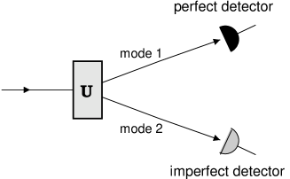
Figure 1: Schematic of the heralded-photon setup.

Suppose now the photon number in the mode 1 is measured by the perfect detector and the photon number in the mode 2 is measured by the imperfect detector. It is now simple to understand the conditional probability of finding $n$ photons in the mode 1, given that $k$ photons are detected in the mode 2. In this way, we can have an operational definition of the conditional probability $Q(n|k)$. It is easy to show that the conditional probability of finding $n$ photons in mode 1 given that $k$ photons are detected in mode 2 is given by precisely the same expression for the quantity $Q(n,k)$ as Eq. (3). [Note that the transformation given by ${\hat{U}}_{H}$ is far from quantum cloning, since the result of $U$ is far from being equal to the cloning transformation $(\sum_{n=0}^{\infty}\alpha_{n}|n\rangle_{1})\otimes(\sum_{n=0}^{\infty}\alpha_{n}|n\rangle_{2})$.

II POVM Description

Suppose an initial quantum state $|\psi_{in}\rangle$ of incident light is represented in the photon number states, as

$$|\psi_{in}\rangle=\sum_{n=0}^{\infty}\alpha_{n}|n\rangle.$$ (5)

The probability of finding $n$ photons is then given by $S(n)=|\langle n|\psi\rangle|^{2}=|\alpha_{n}|^{2}$. We may describe the detection process of the perfect detector by entangling the source with the detector ancilla $|0\rangle$

$$|\psi_{f}\rangle={\hat{U}}|\psi_{in}\rangle|0\rangle=\sum_{n}\alpha_{n}|n\rangle_{Q}|a_{n}\rangle_{M}\;,$$ (6)

where

$${\hat{U}}=\sum_{j}|j\rangle\langle j|\otimes\frac{1}{\sqrt{j!}}({\hat{a}}^{\dagger})^{j}$$ (7)

is the unitary operator implementing the von Neumann measurement, and we identified the quantum ($Q$) and measurement device $(M)$ Hilbert spaces with appropriate subscripts.

The probability to detect $k$ photons, $P(k)$, can now be calculated as

$$P(k)={\rm Tr}_{Q}(|a_{k}\rangle_{M}\langle a_{k}||\psi_{f}\rangle\langle\psi_{fi}|)=|\alpha_{k}|^{2}\;,$$ (8)

as expected. Of course, the same result would have been obtained as $P(k)={\rm Tr}(M_{k}\rho_{in})$ using a Positive Operator Valued Operator Measure (POVM)

$$M_{k}=|k\rangle\langle k|\;.$$ (9)

The present unitary treatment, however, is more transparent and allows a straightforward extension to imperfect detectors.

For an imperfect photodetector with a finite quantum efficiency, the POVM can be written as

$$M_{k}=\sum_{n=k}^{\infty}P(k|n)|a_{n}\rangle\langle a_{n}|,$$ (10)

with $P(k|n)$ given by Eq. (2). We can verify this by calculating as before

$$|\psi_{f}\rangle=U|\psi_{in}\rangle|0\rangle_{M}|0\rangle_{E}\;,$$ (11)

except that the entanglement operator $U$ now acts on the joint Hilbert space of the quantum system, a measurement device, and an environment $|0\rangle_{E}$, which is where our lost photons go. Thus, the unitary operator can be given by

$${\hat{U}}=\sum_{j}|j\rangle\langle j|\otimes\frac{1}{\sqrt{j!}}\left(\sqrt{\eta}\,{\hat{a}}^{\dagger}\otimes\mathbbm{1}+e^{i\varphi}\sqrt{1-\eta}\,\mathbbm{1}\otimes{\hat{b}}^{\dagger}\right)^{j}\;,$$

where ${\varphi}$ is an arbitrary phase and $b^{\dagger}$ is the creation operator for the relevant mode of the environment. Similar to Eq. (8), we now have

$$P(k) = {\rm Tr}_{QE}\left(|a_{k}\rangle_{M}\langle a_{k}||\psi_{fi}\rangle\langle\psi_{fi}|\right)$$ (12)

$$= \sum_{n=k}^{\infty}|\alpha_{n}|^{2}{n\choose k}\eta^{k}(1-\eta)^{n-k}\;.$$

supporting our Eq.(10) as the correct POVM. Note that any relative phase information between the photon number states disappeared.

The POVM effectively transfers the initial quantum state of light into a certain quantum state (as a result of $k$-photon detection) by the transformation

$$\rho_{f-k}\equiv M_{k}\rho_{in}\;,$$ (13)

where $\rho_{in}=|\psi_{in}\rangle\langle\psi_{in}|$. The probability that $k$ photons are detected can then also be written as

$$P(k) = {\rm Tr}\left(\rho_{f-k}\right)$$ (14)

$$= {\rm Tr}\left(M_{k}|\psi_{in}\rangle\langle\psi_{in}|\right)$$

$$= \sum_{n}P(k|n)S(n).$$

On the other hand, the joint probability that the source state is $|n\rangle$ and $k$ photons are detected can be expressed by the probability

$$P(n,k) = {\rm Tr}_{E}(\langle n,a_{k}|\psi_{f}\rangle\langle\psi_{f}|n,a_{k}\rangle)$$ (15)

$$= \langle n|\rho_{f-k}|n\rangle=P(k|n)S(n)\;,$$

which defines the quantity $Q(n|k)$ as

$$Q(n|k)\equiv{\langle a_{n}|\rho_{f-k}|a_{n}\rangle\over{\rm Tr}\left(\rho_{f-k}\right)}\;.$$ (16)

In particular, the quantity $Q(n=k|k)$ corresponds to the confidence of the state preparation in a situation that we have more than two modes for the input and the photon number in one of the modes is measured kok01 .

III An Example

Let us take a simple example of an input coherent state in order to see how the value of $Q(n|k)$ behaves. In doing this, we assume that the dark count rate is small enough that we can ignore it, and the quantum efficiency is independent of the number of incident photons.

A coherent state $|\alpha\rangle$ is expressed in terms of number state as $|\alpha\rangle=e^{-|\alpha|^{2}/2}\sum_{n}(\alpha^{n}/\sqrt{n!})|n\rangle$ scully97 . The probability of finding $n$ photons in $|\alpha\rangle$ is then given by a Poisson distribution:

$$S(n)=|\langle n|\alpha\rangle|^{2}={e^{-{\bar{n}}}{\bar{n}}^{n}\over n!},$$ (17)

where ${\bar{n}}=|\alpha|^{2}$. Now the probability of detection of $k$ photons with an imperfect detector is written as scully69

$$P(k) = \sum_{n=k}^{\infty}{n\choose k}\eta^{k}(1-\eta)^{n-k}{e^{-{\bar{n}}}{\bar{n}}^{n}\over n!}$$ (18)

$$= e^{-{\bar{n}}}\sum_{l=0}^{\infty}{{l+k}\choose k}{{\bar{n}}^{l}{\bar{n}}^{k}\over(l+k)!}\eta^{k}(1-\eta)^{l}$$

$$= e^{-{\bar{n}}}{{\bar{n}}^{k}\eta^{k}\over k!}\sum_{l=0}^{\infty}{{\bar{n}}^{l}\over l!}(1-\eta)^{l}$$

$$= e^{-{\bar{n}}}{({\bar{n}}\eta)^{k}\over k!}e^{-{\bar{n}}(1-\eta)}={({\bar{n}}\eta)^{k}\over k!}e^{-{\bar{n}}\eta}.$$

That is, the photon counting statistics are simply a Poisson distribution where the average number of photons detected is the average number of incident photons multiplied by the quantum efficiency of the detector–given by ${\bar{k}}={\bar{n}}\eta$ as expected.

Figure 2: The conditional probability $Q(n|k=1)$ for a coherent state with ${\bar{n}}=1$ as a function of $n$. (a) For detector efficiency $\eta=0.2$, $Q(1|1)=0.45$, $Q(2|1)=0.36$. (b) For detector efficiency $\eta=0.9$, $Q(1|1)=0.90$, $Q(2|1)=0.09$.

Figure 3: The conditional probability $Q(n|k=1)$ for a coherent state with ${\bar{n}}=0.2$ as a function of $n$. (a) For detector efficiency $\eta=0.2$, $Q(1|1)=0.85$, $Q(2|1)=0.14$. (b) For detector efficiency $\eta=0.9$, $Q(1|1)=0.98$, $Q(2|1)=0.02$.

Now let us consider the conditional probability $Q(n|k)$. Using Eq. (3), it is simply found as

$$Q(n|k) = {{n\choose k}\eta^{k}(1-\eta)^{n-k}e^{-{\bar{n}}}{\bar{n}}^{n}/n!\over e^{-{\bar{n}}\eta}({\bar{n}}\eta)^{k}/k!}$$ (19)

$$= {1\over(n-k)!}(1-\eta)^{n-k}e^{-{\bar{n}}(1-\eta)}{\bar{n}}^{n-k}$$

$$= {e^{-{\bar{l}}}\over l!}{\bar{l}}^{~{}l},$$

where $l=n-k$ and ${\bar{l}}={\bar{n}}(1-\eta)$. Therefore, the form of $Q(n|k)$ is again a Poisson distribution as a function of $n-k$ with the average number of photons that fail to register given as ${\bar{n}}(1-\eta)$.

Figure 2 shows the behavior of $Q(n|k)$ as a function of $n$, for the case of coherent state input with ${\bar{n}}=1$, when one photon is detected. We can see that if the quantum efficiency of the detector is 0.2, with the detection of one photon, then the chances are more than 50% that the input contains more than two photons ($Q(1|1)=0.45$). Obviously, $Q(1|1)$ increases for higher values of the quantum efficiency ($Q(1|1)=0.9$ for $\eta=0.9$).

On the other hand, for a given quantum efficiency of the detector, $Q(1|1)$ gets large as the average number of photons in the input decreases. For ${\bar{n}}=0.2$, $Q(1|1)=0.85$ even if the detector efficiency is 0.2, as depicted in Fig. 3. In this case, with the detection of one photon the chances are 85% that the detection result corresponds to the correct value.

IV Reconstruction of Photon-Number Distribution

So far we have seen that we cannot say much about $Q(n|k)$ if we do not know at least the form of $S(n)$. In other words, using an imperfect detector, even after a detection of $k$ photons, we do not gain much information about the number of incident photons without a prior knowledge of the incident field. Hence, the problem comes back to reconstruction of photon number distribution of the incident field, $S(n)$, from the photon counting probability, $P(k)$ by a sequence of identical inputs and measurements. For this purpose, we may write Eq. (2) in a matrix form as

$${\vec{P}}={\bf P}{\vec{S}},$$ (20)

where

$${\vec{P}} = \left(\begin{array}[]{c}P(0)\\ P(1)\\ P(2)\\ \cdot\\ \cdot\end{array}\right),\quad{\vec{S}}=\left(\begin{array}[]{c}S(0)\\ S(1)\\ S(2)\\ \cdot\\ \cdot\end{array}\right)$$ (31)

and each component of the matrix ${\bf P}$ represents the conditional probability $P(k|n)$ as

$$P_{kn}\equiv P(k|n)={n\choose k}\eta^{k}(1-\eta)^{n-k}.$$ (32)

Then the inverse of ${\bf P}$ can be found explicitly; it is given by

$$(P^{-1})_{nm}={m\choose n}\eta^{-m}(\eta-1)^{m-n}\;,$$ (33)

which, in the absence of dark counts, determines the photon-number distribution of the source from the photon-counting distribution. Note, however, that for a fixed $n$ there are alternating signs in $(P^{-1})_{mn}$ as the index $m$ changes, so that this inversion formula can yield unphysical results depending on the probability distribution $P(k)$. Put another way, for small efficiencies the matrix $\bf P$ is ill-conditioned and ${\bf P}^{-1}$ will contain matrix elements that can get very large in absolute value and can have either sign. This means that even if the calculated $S(n)$’s are all non-negative, a good inversion is still not guaranteed, since the inversion formula (33) is highly sensitive to small changes of $P(k)$, amplifying the statistical and other noise which is inevitably present in any actual measurement. The fact that the inverse matrix $P^{-1}$ is also a upper triangular matrix implies that $S(n)$ is determined by $P(k)$ with $k\geq n$. In other words, the tail of the measurement result, $P(k)$, where the statistical noise can be expected to be greatest, affects the inversion significantly. The validity conditions for the inversion formula shall be discussed elsewhere.

Instead, we can carry out the following recipe: 1) Seek an underlying distribution ${\vec{S}}$ for which ${\bf P}{\vec{S}}$ matches the observed frequencies according to a $\chi^{2}$ goodness-of-fit test. 2) Then, of all such distributions, seek the one with maximum entropy; i.e., pick the most likely underlying distribution, which is statistically consistent with the data. Such a strategy can be implemented as a genetic algorithm, which we will discuss in a forthcoming paper yurtsever03 . Using this method, the reconstruction of ${\vec{S}}$ with a data set from an actual experiment is depicted in Fig. 4. The plot in Fig. 4a shows the probability distribution of the detected photons. The raw count data was normalized by the total number of counts (data provided courtesy of NIST miller03 . The result of reconstruction is shown by the plot Fig. 4b, and yield a ${\bar{n}}=20.15$ for the incident coherent state–a good agreement with the experimental value of ${\bar{n}}_{\rm exp}=4.02$ miller03 .

Figure 4: Reconstruction of the input-state photon-number distribution: (a) Photon counting distribution from the NIST experiment miller03 ; (b) Reconstruction of the input state photon distribution (${\bar{n}}\approx 20.15$), assuming a quantum efficiency of 0.2 and no dark counts.

V Dark Counts

In addition to the finite quantum efficiency, the dark counts further make the results extracted from the experiment obscure. For a constant dark-count rate, however, a generalization of the inversion may be handled analytically. Suppose in general that the probability of $d$ dark counts is $D(d)$, a discrete probability distribution which satisfies the normalization condition

$$\sum_{d=0}^{\infty}D(d)=1\;.$$ (34)

We assume that the distribution $D(d)$ represents probabilities of dark counts in a fixed interval of time $\tau$ (duration of a single photon-counting experiment), and that these probabilities are independent of all other relevant observables such as incoming photon number, number of detected photons, etc. Therefore in the presence of dark counts, the conditional probability of detecting $k$ photons, given $n$ photons in the incident field Eq. (2), is modified accordingly:

$$P_{D}(k|n)=\sum_{d=0}^{k}D(d){n\choose k-d}\eta^{k-d}(1-\eta)^{n-k+d}\;,$$ (35)

which expresses the probability $P_{D}(k|n)$ as a sum (over all possible $d$) of the probability of registering $k-d$ photons from the incident field via true detection while the remaining $d$ are registered via dark-count events.

As long as the physical time scale for the emergence of a dark-count event is much smaller than $\tau$, and the events arrive at a constant rate $\lambda$, the probability distribution $D(d)$ (of the arrival of $d$ dark-count events in the fixed time interval $\tau$) has a Poissonian-distribution limit:

$$D(d)=e^{-\lambda\tau}\frac{(\lambda\tau)^{d}}{d!}\;,$$ (36)

where the average number of dark count is ${\bar{d}}=\lambda\tau$. Since after interchanging the summation index $d$ with $k-d$ we can rewrite Eq. (35) as

$$P_{D}(k|n)=\sum_{d=0}^{k}D(k-d){n\choose d}\eta^{d}(1-\eta)^{n-d}\;,$$ (37)

where the summation over $d$ is in the form of a matrix multiplication [Eq. (32)],

$$(P_{D})_{kn}=\sum_{d}D_{kd}\;P_{dn},\;$$ (38)

or in matrix notation,

$${\bf P_{D}}={\bf D}\,{\bf P}\;,$$ (39)

where $(P_{D})_{kn}\equiv P_{D}(k|n)$, and

$$D_{kd} \equiv D(k-d)$$ (40)

$$= e^{-\lambda\tau}\frac{(\lambda\tau)^{k-d}}{(k-d)!}\;.$$

Throughout the paper, we adopt the convention that $k!=\Gamma(k+1)\equiv\infty$ for negative integer $k$, and correspondingly ${a\choose b}\equiv 0$ whenever $b>a$. In Eq. (40), this convention implies that $D_{kd}=0$ for $d>k$.

Now by inverting Eq. (37) in a matrix form, from the fundamental equation,

$$P(k)=\sum_{n}P_{D}(k|n)\,S(n)\;,$$ (41)

we can reconstruct the photon number distribution $S(n)$ of the incident field given the vector of observed photon-count probabilities $P(k)$, whose relationship to $S(n)$ [given by Eq. (41)], can again be written in matrix form as $\vec{P}={\bf P_{D}}\vec{S}$, just as in Eqs. (20)–(21). The inverse of the coefficient matrix $P_{D}(k|n)=(P_{D})_{kn}$ is found from Eq. (39),

$${\bf P_{D}}^{-1}={\bf P}^{-1}\,{\bf D}^{-1}\;.$$ (42)

Let us first consider the inverse of the matrix ${\bf D}$ defined as in Eq. (30). It is not difficult to prove that the inverse of ${\bf D}$ is given by

$$(D^{-1})_{ij} = e^{\lambda\tau}\frac{(-\lambda\tau)^{i-j}}{(i-j)!}$$ (43)

$$= e^{\lambda\tau}\,(-1)^{i-j}\,\frac{(\lambda\tau)^{i-j}}{(i-j)!}\;.$$

Combining Eq. (33) with Eq. (32) and Eq. (23), we find

$$({P_{D}}^{-1})_{kn} = e^{\lambda\tau}\sum_{i}{i\choose k}\eta^{-i}(\eta-1)^{i-k}\frac{(-\lambda\tau)^{i-n}}{(i-n)!}$$

$$= \frac{(-1)^{k+n}e^{\lambda\tau}}{(1-\eta)^{k}(\lambda\tau)^{n}}\sum_{i=0}^{\infty}\frac{{i\choose k}}{(i-n)!}\left[\frac{(1-\eta)\lambda\tau}{\eta}\right]^{i}\;.$$

The infinite power series over $i$ in Eq. (34) is absolutely convergent for all values of the argument

$$z\equiv\frac{(1-\eta)\lambda\tau}{\eta}\;,$$ (45)

and can be expressed in terms of the generalized hyper-geometric function ${}_{1}\!F_{1}(a,b,z)$ (which is an entire function of the argument $z$ for all parameter values $a$, $b$), giving a compact expression for the inverse matrix elements in the form:

$$({P_{D}}^{-1})_{kn}=(-1)^{k+n}\frac{e^{\lambda\tau}}{(1-\eta)^{k}(\lambda\tau)^{n}}\times$$

$$\left\{\begin{array}[]{ll}\frac{n!}{k!(n-k)!}\;z^{n}\;\,{{}_{1}\!F_{1}}(n+1,\,n-k+1,\,z)&\;\;\textrm{if $k\leqslant n\;,$}\\ \\ \frac{\,1\,}{\,\;(k-n)!\;\,}\;z^{k}\;\,{{}_{1}\!F_{1}}(k+1,\,k-n+1,\,z)&\;\;\textrm{if $k>n\;.$}\end{array}\right.$$ (49)

(50)

The inversion of Eq. (32) can now be effected by substituting Eqs. (35)–(36) into the matrix formula

$$S(k)=\sum_{n}({P_{D}}^{-1})_{kn}\,P(n)\;.$$ (51)

This suggests that the reconstruction of the photon statistics of the source may be possible with any given quantum efficiency of the detector, even in presence of dark counts yurtsever03 . However, as the efficiency falls and the dark-count rate grows, more and more data points will be required for the inversion.

VI Summary

We have shown a way of quantifying the capability of photon-number discriminating detectors by the conditional probability, $Q(n|k)$, given in Eq. (3). This conditional probability, however, can be obtained only when a priori knowledge of the input is available. Without a prior knowledge of the input state the results of photodetection can only eliminate the possibility of having certain numbers of photons in the source rather than determine them in the absence of dark counts. Hence, the term non-photon number-discriminating detector corresponds to the situation where the input state is unknown. On the other hand, the same photodetector could be a photon number-discriminating detector if the input state is known. Of course, the number resolving capability, without a prior knowledge of the input, can be measured qualitatively using the conditional probability $P(k|n)$ of Eq. (2), which is given by the characteristics of the detector itself. In particular, $C_{k}\equiv P(k|K)$ may serve the measure of that capability. For the detector model considered in this paper, the number-resolving capability up to two photons can be written as $C_{k=2}=\eta^{2}$, and for $C_{2}$ to be bigger than 0.5, $\eta$ should be bigger than $1/\sqrt[2]{2}\approx 0.71$. Similarly, $P_{D}(k|k)$ of Eq. (37) plays the same role in the presence of dark counts. For example, with a given dark-count rate $\lambda\tau=0.5$, the detector efficiency $\eta$ should be more than 0.78 for $P_{D}(k|k)$ to be larger than one half.

We then introduced a simple matrix inversion formula in order to reconstruct the input-state photon distribution from the measured photon counting distribution. Due to the form of the inverse matrix and its high sensitivity to the fluctuation, restrictions need to be imposed on the use of this inversion formalism. Alternatively, we can use a genetic algorithm that finds the distribution with maximum entropy after passing the $\chi^{2}$ goodness-of-fit test. We have shown good results for the reconstruction of the input distribution using the data from a recent experiment at NIST. Finally, we have considered the reconstruction task in presence of dark counts and derived a completely analytic formula for the inversion. A detailed analysis of the conditions for the inversion formula to be applicable will be discussed in future work.

References

- (1) E. Knill, R. Laflamme, and G.J. Milburn, Nature, 409, 46 (2001).
- (2) T.B. Pittman, B.C. Jacobs, and J.D. Franson, Phys. Rev. Lett. 88, 257902 (2002).
- (3) J.D. Franson, M.M. Donegan, M.J. Fitch, B.C. Jacobs, and T.B. Pittman, Phys. Rev. Lett. 89, 137901 (2002).
- (4) T.C. Ralph et al., “Quantum computation with optical coherent states,” quant-ph/0306004.
- (5) H. Lee, P. Kok, N.J. Cerf, and J.P. Dowling, Phys. Rev. A 65, 030101 (2002).
- (6) P. Kok, H. Lee, and J.P. Dowling, Phys. Rev. A 65, 052104 (2002).
- (7) J. Fiurásek, Phys. Rev. A 65, 053818 (2002).
- (8) C.C. Gerry, A. Benmoussa, and R.A. Campos, Phys. Rev. A 66, 013804 (2002).
- (9) G.J. Pryde and A.G. White, “Creation of maximally entangled photon number states using optical fibre multiports,” quant-ph/0304135.
- (10) G. Gilbert and M. Hamrick, “Practical quantum crytography: A comprehensive analysis (part one),” MITRE Technical Report (McLean, VA, 2000), quant-ph/0009027.
- (11) N. Gisin, G. Ribordy, W. Tittel, and H. Zbinden, “Quantum cryptography,” Rev. Mod. Phys. 74, 145 (2002).
- (12) J. Kim, S. Takeuchi, and Y. Yamamoto, Appl. Phys. Lett. 74, 902 (1999).
- (13) S. Takeuchi, J. Kim, Y. Yamamoto, and H.H. Hogue, Appl. Phys. Lett. 74, 1063 (1999).
- (14) K. Banaszek and I.A. Wamsley, Opt. Lett. 28, 52 (2003).
- (15) O. Haderka, M. Hamar, and J. Perina Jr., “Experimental multi-photon–resolving detector using a single avalanche photodiode,” quant-ph/0302154.
- (16) J. Rehacek et al., “Multi-photon resolving fiber-loop detector,” quant-ph/0303032.
- (17) D. Achilles et al., “Fiber-assisted detection with photon number resolution,” quant-ph/0305191.
- (18) M.J. Fitch, B.C. Jacobs, T.B. Pittman, and J.D. Franson, “Photon number resolution using a time-multiplexed single-photon detector,” quant-ph/0305193.
- (19) A.J. Miller, S.W. Nam, J.M. Martinis, and A.V. Sergienko, Appl. Phys. Lett. 83, 791 (2003).
- (20) S. Song, C.M. Caves, and B. Yurke, Phys. Rev. A 41, R5261 (1990).
- (21) H. Paul, P. Torma, T. Kiss, and I. Jex, Phys. Rev. Lett. 76, 2464 (1996).
- (22) P. Kok and S.L. Braunstein, Phys. Rev. A 63, 033812 (2001).
- (23) P. Kok, “Limitations on building single-photon–resolution detection devices,” quant-ph/0303102.
- (24) S.D. Bartlett, E. Diamanti, B.C. Sanders, and Y. Yamamoto, “Photon counting schemes and performance of non-deterministic nonlinear gates in linear optics,” quant-ph/0204073.
- (25) L. Mandel, Proc. Phys. Soc. 72, 1037 (1958).
- (26) P.L. Kelley and W.H. Kleinner, Phys. Rev. 136, A316 (1964).
- (27) R.J. Glauber, “Optical Coherence and Photon Statistics,” in Quantum Optics and Electronics, Les Houches 1964, ed. C. DeWitt, A. Blandin, and C. Cohen-Tannoudji, p63 (Gordon and Breach, New York, 1965).
- (28) M.O. Scully and W.E. Lamb, Jr., Phys. Rev. 179, 368 (1969).
- (29) M.O. Scully and M.S. Zubairy, Quantum Optics (Cambridge University Press, Cambridge, UK, 1997).
- (30) U.H. Yurtsever, S.L. Braunstein, G.M. Hockney, P. Kok, H. Lee, C. Adami, and J.P. Dowling (unpublished).