Determination of continuous variable entanglement by purity measurements

Abstract

We classify the entanglement of two–mode Gaussian states according to their degree of total and partial mixedness. We derive exact bounds that determine maximally and minimally entangled states for fixed global and marginal purities. This characterization allows for an experimentally reliable estimate of continuous variable entanglement based on measurements of purity.

Quantum entanglement of Gaussian states constitutes a fundamental resource in continuous variable (CV) quantum information Book . Therefore, the quest for a theoretically satisfying and experimentally realizable quantification of the entanglement for such states stands as a major issue in the field. On the theoretical ground, a proper, computable quantitative characterization of the entanglement of Gaussian states is provided by the logarithmic negativity werner . Experimental schemes to determine the entanglement of Gaussian states have been proposed both in the two–mode kim and in the multipartite vloock instance. However, these schemes are based on homodyne detections, and require a full reconstruction of all the second moments of the Gaussian field.

In this work, we present a theoretical framework to estimate the entanglement of two–mode Gaussian states by the knowledge of the total and of the two partial purities. This is achieved by deriving analytical a priori upper and lower bounds on the logarithmic negativity for fixed values of the global and marginal purities. We then show that the set of entangled Gaussian states is tightly contained between two extremal surfaces of maximally and minimally entangled states. This quantification allows for a simple strategy to measure the entanglement of Gaussian states with reliable experimental accuracy. In fact, measurements of global and marginal purities do not require the demanding reconstruction of the full covariance matrix and can be performed directly by exploiting the technology of quantum networks network .

Let us consider a two–mode continuous variable system, described by the Hilbert space ${\cal H}={\cal H}_{1}\otimes{\cal H}_{2}$ resulting from the tensor product of the Fock spaces ${\cal H}_{k}$’s. We denote by $a_{k}$ the annihilation operator acting on the space ${\cal H}_{k}$. Likewise, $\hat{x}_{k}=(a_{k}+a^{{\dagger}}_{k})/\sqrt{2}$ and $\hat{p}_{k}=-i(a_{k}-a^{{\dagger}}_{k})/\sqrt{2}$ are the quadrature phase operators of the mode $k$, the corresponding phase space variables being $x_{k}$ and $p_{k}$.

In the following, we will make use of the Wigner quasi–probability representation $W(x_{i},p_{i})$, defined as the Fourier transform of the symmetrically ordered characteristic function. In Wigner phase space picture, the tensor product ${\cal H}={\cal H}_{1}\otimes{\cal H}_{2}$ results in the direct sum $\Gamma=\Gamma_{1}\oplus\Gamma_{2}$ of the related phase spaces $\Gamma_{i}$’s. A symplectic transformation acting on the global phase space $\Gamma$ corresponds to a unitary operator acting on $\cal H$ simon . We will refer to a transformation $S_{l}=S_{1}\oplus S_{2}$, with each $S_{i}\in Sp_{(2,\mathbb{R})}$ acting on $\Gamma_{i}$, as to a “local symplectic operation”, corresponding to a “local unitary transformation” $U_{l}=U_{1}\otimes U_{2}$. The set of Gaussian states is defined as the set of states with Gaussian Wigner function

$$W(X)=\frac{\,{\rm e}^{-\frac{1}{2}X\boldsymbol{\sigma}^{-1}X^{T}}}{\pi\sqrt{{\rm Det}\,\boldsymbol{\sigma}}}{\>,}$$ (1)

where $X\equiv(x_{1},p_{1},x_{2},p_{2})\in\Gamma$, and we will denote by $\hat{X}$ the vector of operators $(\hat{x}_{1},\hat{p}_{1},\hat{x}_{2},\hat{p}_{2})$. First moments have been neglected, since they can be set to zero by means of a local unitary transformation. Second moments form the covariance matrix $\boldsymbol{\sigma}$ of the Gaussian state $\sigma_{ij}\equiv\frac{1}{2}\langle\hat{X}_{i}\hat{X}_{j}+\hat{X}_{j}\hat{X}_{i}\rangle-\langle\hat{X}_{i}\rangle\langle\hat{X}_{j}\rangle$. For simplicity, in what follows $\boldsymbol{\sigma}$ will refer both to the Gaussian state and to its covariance matrix. It is convenient to express $\boldsymbol{\sigma}$ in terms of the three $2\times 2$ matrices $\boldsymbol{\alpha}$, $\boldsymbol{\beta}$, $\boldsymbol{\gamma}$

$$\boldsymbol{\sigma}\equiv\left(\begin{array}[]{cc}\boldsymbol{\alpha}&\boldsymbol{\gamma}\\ \boldsymbol{\gamma}^{T}&\boldsymbol{\beta}\end{array}\right)\,.$$ (2)

Heisenberg uncertainty principle can be expressed as simon

$$\boldsymbol{\sigma}+\frac{i}{2}\boldsymbol{\Omega}\geq 0\;,$$ (3)

where $\boldsymbol{\Omega}\equiv\boldsymbol{\omega}\oplus\boldsymbol{\omega}$ is the usual symplectic form with $\omega_{ij}=\delta_{ij-1}-\delta_{ij+1}$, $i,j=1,2$. Ineq. (3) can be recast as a constraint on the $Sp_{(4,{\mathbb{R}})}$ invariants $\Delta\equiv\,{\rm Det}\,\boldsymbol{\alpha}+\,{\rm Det}\,\boldsymbol{\beta}+2\,{\rm Det}\,\boldsymbol{\gamma}$, and ${\rm Det}\,\boldsymbol{\sigma}$ simon

$$\Delta\leq\frac{1}{4}+4\,{\rm Det}\,\boldsymbol{\sigma}\,.$$ (4)

In general, the Wigner function transforms as a scalar under symplectic operations, while the covariance matrix $\boldsymbol{\sigma}$ transforms according to $\boldsymbol{\sigma}\rightarrow S^{T}\boldsymbol{\sigma}S$, with $S\in Sp_{(4,\mathbb{R})}$. As it is well known duan , for any covariance matrix $\boldsymbol{\sigma}$ there exists a local canonical operation $S_{l}=S_{1}\oplus S_{2}$ that recasts $\boldsymbol{\sigma}$ in the “standard form” $\boldsymbol{\sigma}_{sf}$ with $\boldsymbol{\alpha}=\,{\rm diag}\,\{a,a\}$, $\boldsymbol{\beta}=\,{\rm diag}\,\{b,b\}$, $\boldsymbol{\gamma}=\,{\rm diag}\,\{c_{+},c_{-}\}$, where $a$, $b$, $c_{+}$, $c_{-}$ are determined by the four local symplectic invariants ${\rm Det}\,\boldsymbol{\sigma}$, ${\rm Det}\,\boldsymbol{\alpha}$, ${\rm Det}\,\boldsymbol{\beta}$, and ${\rm Det}\,\boldsymbol{\gamma}$.

Any bipartite Gaussian state $\boldsymbol{\sigma}$ can always be written as $\boldsymbol{\sigma}=S^{T}\boldsymbol{\nu}S$ for some $S\in Sp_{4,\mathbb{R}}$ and $\boldsymbol{\nu}=\,{\rm diag}\,\{n_{-},n_{-},n_{+},n_{+}\}$. The quantities $n_{\mp}$ constitute the symplectic spectrum of $\boldsymbol{\sigma}$; they are determined by the global symplectic invariants holevo ; sirkaz

$$2n_{\mp}^{2}=\Delta\mp\sqrt{\Delta^{2}-4\,{\rm Det}\,\boldsymbol{\sigma}}\,.$$ (5)

In terms of $n_{\mp}$ Ineq. (4) becomes simply $n_{-}\geq 1/2$.

We will characterize the mixedness of a quantum state $\varrho$ by its purity $\mu\equiv\,{\rm Tr}\,\varrho^{2}$. For a $n$–mode Gaussian state $\boldsymbol{\sigma}$ the purity is simply evaluated integrating the Wigner function, yielding $\mu=1/(2^{n}\,\sqrt{{\rm Det}\,\boldsymbol{\sigma}})$.

As for the entanglement, we recall that the positivity of the partially transposed (PPT) state $\tilde{\boldsymbol{\sigma}}$ is equivalent to separability for any two–mode Gaussian state $\boldsymbol{\sigma}$ simon . In terms of symplectic invariants, partial transposition corresponds to flipping the sign of ${\rm Det}\,\boldsymbol{\gamma}$, so that $\Delta$ turns into $\tilde{\Delta}=\Delta-4\,{\rm Det}\,\boldsymbol{\gamma}$. The symplectic spectrum $\tilde{n}_{\mp}$ of $\tilde{\boldsymbol{\sigma}}$ is simply found inserting $\tilde{\Delta}$ for $\Delta$ in Eq. (5). If $\tilde{n}_{-}$ is the smallest symplectic eigenvalue of the partially transposed covariance matrix $\tilde{\boldsymbol{\sigma}}$, a state $\boldsymbol{\sigma}$ is separable if and only if

$$\tilde{n}_{-}\geq 1/2\;.$$ (6)

A bona fide measure of entanglement for two–mode Gaussian states should thus be a monotonically decreasing function of $\tilde{n}_{-}$, quantifying the violation of inequality (6). A computable entanglement monotone for generic two-mode Gaussian states is provided by the logarithmic negativity $E_{{\cal N}}=\max\{0,-\ln(2\tilde{n}_{-})\}$ werner . For symmetric Gaussian states, i.e. states whose standard form is characterized by $\boldsymbol{\alpha}=\boldsymbol{\beta}$, another computable entanglement monotone is provided by the entanglement of formation giedke . However, in this subcase the two measures provide the same characterization of entanglement and are fully equivalent. Therefore, from now on we will adopt the logarithmic negativity to quantify the entanglement of two-mode Gaussian states.

We now show that a generic state in standard form can be reparametrized in terms of the $Sp_{(4,\mathbb{R})}$ invariants $\mu$ (the global purity) and $\Delta$, and of the $Sp_{(2,\mathbb{R})}\oplus Sp_{(2,\mathbb{R})}$ invariants $\mu_{1}$ and $\mu_{2}$, where $\mu_{i}$ denotes the purity of the reduced state in mode $i$ ($i=1,2$). For a generic two-mode Gaussian state $\boldsymbol{\sigma}_{sf}$ we thus have

$$\mu_{1} = \frac{1}{2a}\,,\quad\mu_{2}\,\,=\,\,\frac{1}{2b}\,,$$ (7)

$$\frac{1}{16\mu^{2}} = {\rm Det}\,{\boldsymbol{\sigma}}=(ab)^{2}-ab(c_{+}^{2}+c_{-}^{2})+(c_{+}c_{-})^{2}\,,$$ (8)

$$\Delta = a^{2}+b^{2}+2c_{+}c_{-}\,.$$ (9)

Eqs. (7-9) are easily inverted to provide the following parametrization

$$a = \frac{1}{2\mu_{1}}\,,\quad b\,\,=\,\,\frac{1}{2\mu_{2}}\,,$$ (10)

$$c_{\pm} = \frac{1}{2}\sqrt{\mu_{1}\mu_{2}\left[\left(\Delta-\frac{(\mu_{1}-\mu_{2})^{2}}{4\mu_{1}^{2}\mu_{2}^{2}}\right)^{2}-\frac{1}{4\mu^{2}}\right]}\;\pm\,\epsilon$$

$${\rm with}\quad\epsilon\,\equiv\,\frac{1}{8}\sqrt{\frac{\left[(\mu_{1}+\mu_{2})^{2}-4\mu_{1}^{2}\mu_{2}^{2}\Delta\right]^{2}}{\mu_{1}^{3}\mu_{2}^{3}}-\frac{4\mu_{1}\mu_{2}}{\mu^{2}}}\,.$$

The global and marginal purities range from $0$ to $1$, constrained by the condition

$$\mu\geq\mu_{1}\mu_{2}\;,$$ (12)

a direct consequence of Heisenberg uncertainty relations. It implies that no Gaussian LPTP (less pure than product) states exist, at variance with the case of two–qubit systems adesso . Eqs. (5,10, LABEL:gc) determine the smallest symplectic eigenvalue of the covariance matrix $\boldsymbol{\sigma}$ and of its partial transpose $\tilde{\boldsymbol{\sigma}}$

$$2n_{-}^{2}=\Delta-\sqrt{\Delta^{2}-{\frac{1}{4\mu^{2}}}}\,,\quad 2\tilde{n}_{-}^{2}=\tilde{\Delta}-\sqrt{\tilde{\Delta}^{2}-{\frac{1}{4\mu^{2}}}}\,,$$ (13)

where $\tilde{\Delta}=-\Delta+1/2\mu_{1}^{2}+1/2\mu_{2}^{2}$. This parametrization describes physical states if the radicals in Eqs. (LABEL:gc, 13) exist and Ineq. (4), expressing the Heisenberg principle, is satisfied. All these conditions can be combined and recast as upper and lower bounds on the invariant $\Delta$

$$\frac{1}{2\mu}+\frac{(\mu_{1}-\mu_{2})^{2}}{4\mu_{1}^{2}\mu_{2}^{2}}\,\,\leq\,\,\Delta$$ (14)

$$\leq \min\left\{\frac{(\mu_{1}+\mu_{2})^{2}}{4\mu_{1}^{2}\mu_{2}^{2}}-\frac{1}{2\mu}\;,\;\frac{1}{4}\left(1+\frac{1}{\mu^{2}}\right)\right\}\,.$$

The invariant $\Delta$ has a direct physical interpretation: at given global and marginal purities, it determines the amount of entanglement of the state. In fact, one has

$$\left.\frac{\partial\ \tilde{n}^{2}_{-}}{\partial\ \Delta}\right|_{\mu_{1},\,\mu_{2},\,\mu}\,=\;\frac{1}{2}\left(\frac{\tilde{\Delta}}{\sqrt{\tilde{\Delta}^{2}-{\frac{1}{4\mu^{2}}}}}-1\right)\,>0\,.$$ (15)

The smallest symplectic eigenvalue of the partially transposed state is strictly monotone in $\Delta$. Therefore the entanglement of a generic Gaussian state $\boldsymbol{\sigma}$ with global purity $\mu$ and marginal purities $\mu_{1,2}$ strictly increases with decreasing $\Delta$. Since $\Delta$ has both lower and upper bounds, due to Ineq. (14), not only maximally but also minimally entangled Gaussian states exist. This is an important result concerning the relation between entanglement and purity of quantum states: the entanglement of a Gaussian state is tightly bound by the amount of global and marginal purities, with only one remaining degree of freedom related to the invariant $\Delta$.

We now aim to characterize extremal (maximally or minimally) entangled Gaussian states for fixed global and marginal purities. Let us first consider the states saturating the lower bound in Eq. (14), which entails maximal entanglement. They are Gaussian maximally entangled mixed states (GMEMS), admitting the following parametrization

$$a=\frac{1}{2\mu_{1}},\;b=\frac{1}{2\mu_{2}},\;c_{\pm}=\pm\frac{1}{2}\sqrt{\frac{1}{\mu_{1}\mu_{2}}-\frac{1}{\mu}}\;.$$ (16)

We now recall that Gaussian squeezed thermal states are states of the form $\boldsymbol{\sigma}=S_{r}\boldsymbol{\nu}S_{r}$, where $S_{r}$ is the symplectic representation of the two–mode squeezing operator ${\rm Exp}\,[r(a_{1}a_{2}-a_{1}^{{\dagger}}a_{2}^{{\dagger}})/2]$, while $\boldsymbol{\nu}=\,{\rm diag}\,\{n_{-},n_{-},n_{+},n_{+}\}$. These states are in standard form with $a=n_{-}\cosh^{2}r+n_{+}\sinh^{2}r$, $b=n_{+}\cosh^{2}r+n_{-}\sinh^{2}r$, $\;c_{+}=-c_{-}=(n_{-}+n_{+})\sinh 2r/2$. In the pure case ($n_{\mp}=1/2$) they reduce to two–mode squeezed vacua. We thus find that states of the form of Eq. (16) are non–symmetrical squeezed thermal states with $\tanh 2r=(\mu_{1}\mu_{2}-\mu_{1}^{2}\mu_{2}^{2}/\mu)^{1/2}/(\mu_{1}+\mu_{2})$. These states are separable in the range

$$\mu\leq\frac{\mu_{1}\mu_{2}}{\mu_{1}+\mu_{2}-\mu_{1}\mu_{2}}\,.$$ (17)

In such a separable region in the space of purities, no entanglement can occur for states of the form of Eq. (16), while, outside this region, they are GMEMS. We now consider the class of states that saturate the upper bound in Eq. (14). They determine the class of Gaussian least entangled mixed states (GLEMS). Violation of Ineq. (17) implies that $\left(1+1/\mu^{2}\right)/4\leq(\mu_{1}+\mu_{2})^{2}/4\mu_{1}^{2}\mu_{2}^{2}-1/2\mu$. Therefore, outside the separable region, GLEMS fulfill

$$\Delta=\frac{1}{4}\left(1+\frac{1}{\mu^{2}}\right)\,.$$ (18)

Eq. (18) expresses saturation of Heisenberg relation (4). We thus find that the most semiclassical states of minimum quantum uncertainty are Gaussian least entangled states. GLEMS in standard form are characterized by

$$c_{\pm}\!\! = \!\!\frac{1}{8}\sqrt{\mu_{1}\mu_{2}\left[-\frac{4}{\mu^{2}}+\left(1+\frac{1}{\mu^{2}}-\frac{(\mu_{1}-\mu_{2})^{2}}{\mu_{1}^{2}\mu_{2}^{2}}\right)^{2}\right]}$$

$$\pm \!\!\frac{1}{8\mu}\sqrt{-4\mu_{1}\mu_{2}+\frac{\left[\left(1+\mu^{2}\right)\mu_{1}^{2}\mu_{2}^{2}-\mu^{2}{\left(\mu_{1}+\mu_{2}\right)}^{2}\right]^{2}}{\mu^{2}\mu_{1}^{3}\mu_{2}^{3}}}\;.$$

According to the PPT criterion, GLEMS are separable only for $\mu\leq\mu_{1}\mu_{2}/\sqrt{\mu_{1}^{2}+\mu_{2}^{2}-\mu_{1}^{2}\mu_{2}^{2}}$, so that in the range

$$\frac{\mu_{1}\mu_{2}}{\mu_{1}+\mu_{2}-\mu_{1}\mu_{2}}<\mu\leq\frac{\mu_{1}\mu_{2}}{\sqrt{\mu_{1}^{2}+\mu_{2}^{2}-\mu_{1}^{2}\mu_{2}^{2}}}$$ (20)

both separable and entangled states can be found. The very narrow region defined by Ineq. (20) is the only coexistence region between entangled and separable Gaussian mixed states. Furthermore, Ineq. (14) leads to the following constraint on the purities

$$\mu\leq\frac{\mu_{1}\mu_{2}}{\mu_{1}\mu_{2}+\left|\mu_{1}-\mu_{2}\right|}\,.$$ (21)

For purities which saturate Ineq. (21), GMEMS and GLEMS coincide and we have a unique class of states depending only on the marginal purities $\mu_{1,2}$. They are Gaussian maximally entangled states for fixed marginals (GMEMMS). The maximal entanglement of a Gaussian state decreases rapidly with increasing difference of marginal purities, in analogy with finite-dimensional systems adesso . For symmetric states $(\mu_{1}=\mu_{2})$ Ineq. (21) reduces to the trivial bound $\mu\leq 1$ and GMEMMS reduce to pure two–mode squeezed states.

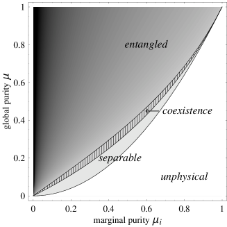
Figure 1: Summary of entanglement properties of symmetric Gaussian states with given global and marginal purities. In the entangled region, the average logarithmic negativity Eq. (25) is depicted, growing from gray to black. The dashed area is the coexistence region of separable and entangled states.

We can summarize the previous results in the following scheme, classifying all the two-mode Gaussian physical states according to their degree of global and marginal purities

$$\mu_{1}\mu_{2}\;\leq\;\mu\;\leq\;\frac{\mu_{1}\mu_{2}}{\mu_{1}+\mu_{2}-\mu_{1}\mu_{2}}\!\! \Rightarrow$$ separable

$$\frac{\mu_{1}\mu_{2}}{\mu_{1}+\mu_{2}-\mu_{1}\mu_{2}}<\mu\leq\frac{\mu_{1}\mu_{2}}{\sqrt{\mu_{1}^{2}+\mu_{2}^{2}-\mu_{1}^{2}\mu_{2}^{2}}}\!\! \Rightarrow$$ coexistence

$$\frac{\mu_{1}\mu_{2}}{\sqrt{\mu_{1}^{2}+\mu_{2}^{2}-\mu_{1}^{2}\mu_{2}^{2}}}<\mu\leq\frac{\mu_{1}\mu_{2}}{\mu_{1}\mu_{2}+\left|\mu_{1}-\mu_{2}\right|}\!\! \Rightarrow$$ entangled

Knowledge of the global and marginal purities thus accurately characterizes the entanglement of Gaussian states, providing strong sufficient conditions and analytical bounds. As we will now show, marginal and global purities allow also an accurate quantification of entanglement. Outside the separable region, GMEMS attain maximum logarithmic negativity $E_{{{\cal N}}max}$

$$E_{{{\cal N}}max}(\mu_{1,2},\mu)=-\frac{1}{2}\log\Bigg{[}-\frac{1}{\mu}+\left(\frac{\mu_{1}+\mu_{2}}{2\mu_{1}^{2}\mu_{2}^{2}}\right)$$

$$\times\left(\mu_{1}+\mu_{2}-\sqrt{(\mu_{1}+\mu_{2})^{2}-\frac{4\mu_{1}^{2}\mu_{2}^{2}}{\mu}}\right)\Bigg{]}\,,$$ (23)

while, in the entangled region (see Eq. (LABEL:entsum)), GLEMS acquire minimum logarithmic negativity $E_{{{\cal N}}min}$

$$E_{{{\cal N}}min}(\mu_{1,2},\mu)=-\frac{1}{2}\log\Bigg{[}\frac{1}{\mu_{1}^{2}}+\frac{1}{\mu_{2}^{2}}-\frac{1}{2\mu^{2}}-\frac{1}{2}$$

$$-\sqrt{\left(\frac{1}{\mu_{1}^{2}}+\frac{1}{\mu_{2}^{2}}-\frac{1}{2\mu^{2}}-\frac{1}{2}\right)^{2}-\frac{1}{\mu^{2}}}\;\Bigg{]}\,.$$ (24)

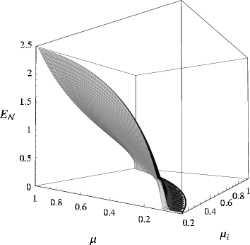
Figure 2: Upper and lower bounds on the logarithmic negativity as functions of the global and marginal purities of symmetric Gaussian states. The black (gray) surface represents GMEMS (GLEMS).

Knowledge of $\Delta$ (i.e. of the full covariance matrix) would allow for an exact quantification of the entanglement. However, we will now show that an estimate based only on the knowledge of the experimentally measurable global and marginal purities turns out to be quite accurate. We can in fact quantify the entanglement of Gaussian states with given global and marginal purities by the “average logarithmic negativity” $\bar{E}_{{\cal N}}$ defined as

$$\bar{E}_{{\cal N}}(\mu_{1,2},\mu)\equiv\frac{E_{{{\cal N}}max}(\mu_{1,2},\mu)+E_{{{\cal N}}min}(\mu_{1,2},\mu)}{2}\;.$$ (25)

We can then also define the relative error $\delta\bar{E}_{{\cal N}}$ on $\bar{E}_{{\cal N}}$ as

$$\delta\bar{E}_{{\cal N}}(\mu_{1,2},\mu)\equiv\frac{E_{Nmax}(\mu_{1,2},\mu)-E_{Nmin}(\mu_{1,2},\mu)}{E_{Nmax}(\mu_{1,2},\mu)+E_{Nmin}(\mu_{1,2},\mu)}\,.$$ (26)

It is easily seen that this error decreases both with increasing global purity and decreasing marginal purities, i.e. with increasing entanglement. For ease of graphical display, let us consider the important case of symmetric Gaussian states, for which the reduction $\mu_{1}=\mu_{2}\equiv\mu_{i}$ occurs.

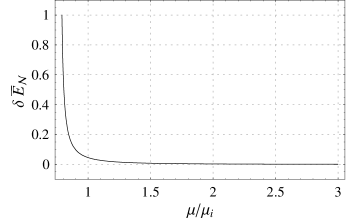
Figure 3: The relative error $\delta\bar{E}_{{\cal N}}$ Eq. (26) on the average logarithmic negativity as a function of the ratio $\mu/\mu_{i}$, plotted at $\mu=0.5$.

Fig. 1 shows the classification of the entanglement of symmetric states depending on their global and marginal purities. Notice in particular the very narrow region of coexistence of separable and entangled states. In Fig. 2, $E_{{{\cal N}}min}(\mu_{i},\,\mu)$ of Eq. (24) and $E_{{{\cal N}}max}(\mu_{i},\,\mu)$ of Eq. (23) are plotted versus $\mu_{i}$ and $\mu$. In the case $\mu=1$ the upper and lower bounds correctly coincide, since for pure states the entanglement is completely quantified by the marginal purity. For mixed states this is not the case, but, as the plot shows, knowledge of the global and marginal purities strictly bounds the entanglement both from above and from below.

The relative error $\delta\bar{E}_{{\cal N}}(\mu_{i},\,\mu)$ given by Eq. (26) is plotted in Fig. 3 as a function of the ratio $\mu/\mu_{i}$. It decays exponentially, and falls below $5\%$ for $\mu>\mu_{i}$. Thus detection of genuinely entangled states is always assured by this method, except at most for a small set of states with very weak entanglement (states with $E_{{\cal N}}\lesssim 1$). Moreover, the accuracy is even greater in the general non-symmetric case $\mu_{1}\neq\mu_{2}$, because the maximal entanglement decreases in such an instance. The above analysis demonstrates that the average logarithmic negativity $\bar{E}_{{\cal N}}$ is a reliable estimate of the logarithmic negativity $E_{{\cal N}}$, improving as the entanglement increases. This allows for an accurate quantification of CV entanglement by knowledge of the global and marginal purities. The latter quantities may be in turn amenable to direct experimental determination by exploiting the technology of quantum networks network , even without homodyningcerf . The present work thus may provide a powerful operative characterization and quantification of the entanglement of generic Gaussian states.

Financial support from INFM, INFN, and MIUR under national project PRIN-COFIN 2002 is acknowledged.

References

(1)Quantum Information Theory with
Continuous Variables, S. L. Braunstein and A. K. Pati
Eds. (Kluwer, Dordrecht, 2002).
(2) G. Vidal and R. F. Werner,
Phys. Rev. A 65, 032314 (2002); J. Eisert, Ph. D.
thesis (University of Potsdam, 2001); K. Życzkowski et al.,
Phys. Rev. A 58, 883 (1998).
(3) M.-S. Kim, J. Lee, and W. J. Munro, Phys. Rev. A 66, 030301(R) (2002).
(4) P. van Loock and A. Furusawa, Phys. Rev. A 67, 052315 (2003).
(5) A. K. Ekert et al., Phys. Rev. Lett. 88, 217901 (2002);
R. Filip, Phys. Rev. A 65, 062320 (2002).
(6) R. Simon, Phys. Rev. Lett. 84, 2726 (2000).
(7) L.-M. Duan, et al.,
Phys. Rev. Lett. 84, 2722 (2000).
(8) A. S. Holevo, M. Sohma, and O. Hirota, Phys. Rev. A 59, 1820 (1999);
A. S. Holevo and R. F. Werner, Phys. Rev. A 63, 032312 (2001).
(9) A. Serafini, F. Illuminati, and S. De Siena, J. Phys. B:
At. Mol. Opt. Phys. 37, L21 (2004).
(10) G. Giedke et al., Phys. Rev. Lett. 91, 107901 (2003).
(11) G. Adesso, F. Illuminati, and S. De Siena, e-print quant-ph/0307192 (2003), and Phys. Rev. A, in press.
(12) J. Fiurasek and N. J. Cerf, e-print quant-ph/0311119 (2003).