Bell Inequalities for Position Measurements

Abstract

Bell inequalities for position measurements are derived using the bits of the binary expansion of position-measurement results. Violations of these inequalities are obtained from the output state of the Non-degenerate Optical Parametric Amplifier.

In the Einstein-Podolsky-Rosen (EPR) paradox devised in Ref. Einstein et al. (1935), a main ingredient is position measurements, and it has been a long-standing controversy whether such measurements together with momentum measurements provide non-local statistics or not. While it certainly is true that the original EPR paper only is intended to ask the question of completeness, many have put considerable thought into the of the possible non-locality of this system. It would seem that this question was put to rest by Bell in Ref. Bell (1986) where he presented a local realist model for position and momentum measurements on the original EPR state, constructed using the Wigner function representation of the EPR state as a joint probability of the measurement results. The Wigner function generally has all the properties of a probability measure except one: it can be negative (a proper probability measure is always positive). However, in this particular case the Wigner function is positive, so it can be used as a proper probability measure.

One could be led to think that this implies that the EPR state can be described by a local realist model, but this is not the case: the important thing to note is the statement “for position and momentum measurements”. That is, nothing is said about other measurements; the quantum state contains more than just information about position and/or momentum. In fact, if one instead uses measurements of parity, one can interpret the Wigner function as a correlation function for these parity measurements, and then certain regularized EPR states are nonlocal, e.g., the Non-degenerate Optical Parametric Amplifier (NOPA) state Banaszek and Wódkiewicz (1998). The next step was taken by Chen et al Chen et al. (2002) who used parity of number to violate a Bell inequality. Finally, in Ref. Larsson (2003) it was shown that the full number operator together with suitable other operators can be used to violate the Bell inequality. The aim of this paper is to show that the position operator itself together with suitable other operators also can be used to violate the Bell inequality, in a sense, deriving a Bell inequality more suited to the original EPR setting.

In the standard Bell inequality there is a bipartite spin-$\tfrac{1}{2}$ system (see e.g., Ref. Bell (1964); Clauser et al. (1969)); at each site a spin-$\tfrac{1}{2}$ measurement is made, and the direction along which the measurement is made constitute a local parameter. In general, this parameter is a direction in space, but in this paper for simplicity only one angular parameter will be retained, in quantum notation,

$$s_{\phi}=\cos\phi\,s_{z}+\sin\phi\,s_{x}$$ (1)

The shorthand notation $s_{\alpha}s^{\prime}_{\gamma}$ will be used to denote the quantum operator $s_{\alpha}\otimes s_{\gamma}$ below. The results of the individual measurements $s_{\alpha}\otimes{}I$ and $I\otimes s_{\gamma}$ will be denoted $S_{\alpha}$ and $S^{\prime}_{\gamma}$. That is, these are the classical $\pm 1$ (“up”/“down”) values registered from each local measurement, e.g., written down on a piece of paper or similar. The question is now if these results can be described under the assumption of local realism:

1. Realism: There is a classical probabilistic model where the results depend on a “hidden variable” $\lambda$, i.e.,

   $$\begin{split}S_{\alpha}&=S_{\alpha}(\lambda),\\ S^{\prime}_{\gamma}&=S^{\prime}_{\gamma}(\lambda).\end{split}$$ (2)

2. Locality: The model is local, such that measurement settings at one site does not affect the other site, i.e.,

   $$\begin{split}S_{\alpha}(\lambda)&\text{ is independent of }\gamma,\\ S^{\prime}_{\gamma}(\lambda)&\text{ is independent of }\alpha.\end{split}$$ (3)

3. Result restriction. The measurement results are restricted in size:

   $$|S_{\alpha}(\lambda)|\leq 1,\quad|S^{\prime}_{\gamma}(\lambda)|\leq 1.$$ (4)

When this is the case, we have the CHSH inequality Clauser et al. (1969)

$$\begin{split}&\big{|}E(S_{\alpha}S^{\prime}_{\gamma})+E(S_{\alpha}S^{\prime}_{\delta})\big{|}+\big{|}E(S_{\beta}S^{\prime}_{\gamma})-E(S_{\beta}S^{\prime}_{\delta})\big{|}\leq 2.\end{split}$$ (5)

This inequality is violated by the entangled state

$$|\psi\rangle=\tfrac{1}{\sqrt{2}}\big{(}|+_{z}+_{z}\rangle+|-_{z}-_{z}\rangle\big{)},$$ (6)

at the settings $\alpha=0$, $\beta=\frac{\pi}{2}$, $\gamma=\frac{\pi}{4}$, and $\delta=-\frac{\pi}{4}$, for which the corresponding quantum expression

$$\big{|}\langle s_{0}s^{\prime}_{\frac{\pi}{4}}\rangle+\langle s_{0}s^{\prime}_{-\frac{\pi}{4}}\rangle\big{|}+\big{|}\langle s_{\frac{\pi}{2}}s^{\prime}_{\frac{\pi}{4}}\rangle-\langle s_{\frac{\pi}{2}}s^{\prime}_{-\frac{\pi}{4}}\rangle\big{|}=2\sqrt{2}>2.$$ (7)

The idea now is to extend this to position measurements. To do this, we choose an interval length $l$, quite arbitrarily for now, and denote the position operator $q$, since the letter $x$ is used for other purposes. Now, let us determine whether or not the measured value of the position $Q$ is in a box of length $l$, at position $nl$ from the origin for integer $n$. This corresponds to an operator $k_{n,l}$ that projects a state $\psi$ (in position representation) onto the subspace of states with support only in $nl\leq q<nl+l$,

$$k_{n,l}\psi(q)=\begin{cases}\psi(q),&nl\leq q<nl+l\\ 0,&\text{otherwise.}\end{cases}$$ (8)

We can now write down an operator that will become the equivalent of a spin-$z$ operator,

$$s_{z,l}=\sum_{n=-\infty}^{\infty}(-1)^{n}k_{n,l}.$$ (9)

So far, this operator only has the same eigenvalues as the usual spin-$z$ operator ($\pm 1$), but the construction can be extended to a full pseudo-spin system. To do this we need spin-step operators, and these can be constructed from a box-translation operator that translates a state $\psi$ by $l$ length units and then projects into the same subspace as used above,

$$t_{n,l}\psi(q) =\begin{cases}\psi(q+l),&nl\leq q<nl+l\\ 0,&\text{otherwise,}\end{cases}$$ (10)

with adjoint

$$t^{{\dagger}}_{n,l}\psi(q) =\begin{cases}\psi(q-l),&nl+l\leq q<nl+2l\\ 0,&\text{otherwise.}\end{cases}$$ (11)

The positive spin-step should take an eigenstate of $s_{z,l}$ with eigenvalue $-1$ to one with eigenvalue $+1$, and its adjoint should do the opposite:

$$s_{+,l}=(s_{-,l})^{{\dagger}}=\sum_{n=-\infty}^{\infty}t_{2n,l}.$$ (12)

Via the usual

$$s_{x,l}=s_{+,l}+s_{-,l},\qquad s_{y,l}=-i(s_{+,l}-s_{-,l})$$ (13)

we have constructed a pseudo-spin system,

$$[s_{x,l},s_{y,l}]=2is_{z,l},\quad\ldots,\quad\text{and}\quad s_{x,l}^{2}=s_{y,l}^{2}=s_{z,l}^{2}=\mathbb{I}.$$ (14)

We can now derive a violation of the simple Bell inequality (5) above from our two-mode Gaussian NOPAstate. In position expansion,

$$\left|\psi_{\text{NOPA}}\right\rangle=\frac{1}{\sqrt{\pi}}e^{qq^{\prime}\sinh 2r-\frac{1}{2}\big{(}q^{2}+(q^{\prime})^{2}\big{)}\cosh 2r}.$$ (15)

By symmetry, measurements along orthogonal directions are uncorrelated at the two sites, e.g., $\langle s_{z,l}s_{x,l}^{\prime}\rangle=0$. The correlations for equal directions must unfortunately be calculated by numeric integration of a two-dimensional Gaussian on $l\times l$ squares. For varying squeezing $r$ and minimal length $l$, we have data as shown in Fig. 1.

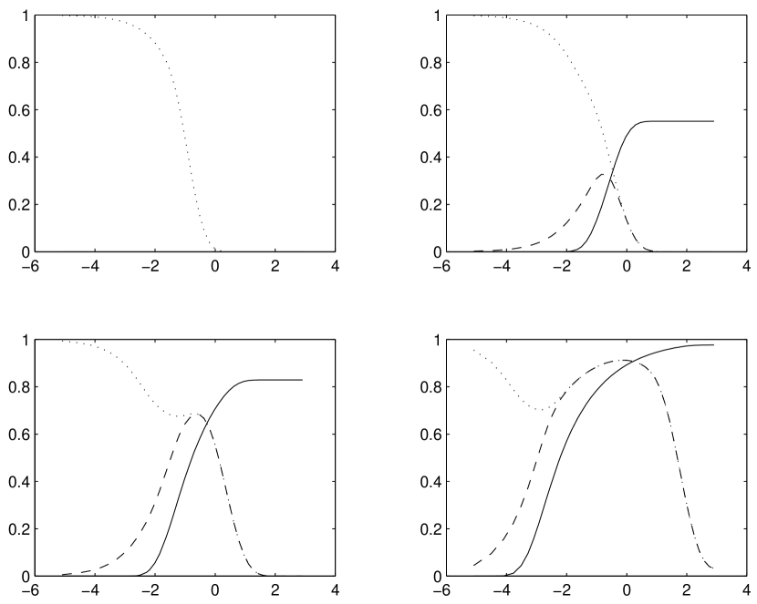
Figure 1: Calculation of $\langle s_{z,l}s_{z,l}^{\prime}\rangle$ (solid line), $\langle s_{x,l}s^{\prime}_{x,l}\rangle$ (dotted line), and $\langle s_{y,l}s^{\prime}_{y,l}\rangle$ (dashed line) for $0.03\leq l\leq 7.5$ (the horizontal scale is logarithmic, i.e., $\log_{2}l$) and $r=0$, $0.5$, $1$, and $2$ from top left to bottom right.

In Fig. 1 there are some interesting features. First, there is a high correlation in the $s_{x,l}$ and $s_{x,l}^{\prime}$ results when $l$ is small. This is perfectly natural from the construction of the operator; it is such that if the wave-function is smooth , then

$$\lim_{l\rightarrow\infty}\langle s_{x,l}\rangle=1.$$ (16)

We have the completely classical property that measurement of $s_{x,l}$ always yields the result 1 at very small $l$. When the squeezing is increased, the slope of the wave function is larger, so that one needs to go to a smaller $l$ to get this effect, but at a given squeezing, there is always an $l$ at which this sets in.

Furthermore, there is a high correlation between $s_{z,l}$ and $s_{z,l}^{\prime}$ when $l$ is large, but for a different reason; note that $\langle s_{z,l}\rangle=0$ for all $l$. When $l$ is large, almost all of the probability falls into the four $l\times l$ squares around the origin. When the wave function is squeezed, more probability falls into the two boxes where the $s_{z}$ and $s_{z}^{\prime}$ results are the same. For fixed squeezing $r$, the limit for large $l$ can be calculated explicitly as

$$\lim_{l\rightarrow\infty}\langle s_{z,l}s_{z,l}^{\prime}\rangle=\frac{2}{\pi}\arctan\big{(}\sinh(2r)\big{)}.$$ (17)

This value corresponds well with the values seen in Fig. 1.

The interesting regime is where all three correlations $\langle s_{x,l}s_{x,l}^{\prime}\rangle$, $\langle s_{y,l}s_{y,l}^{\prime}\rangle$, and $\langle s_{z,l}s_{z,l}^{\prime}\rangle$ are high, remember that the state in Eq. (6) has $\langle s_{x}s_{x}^{\prime}\rangle=\langle s_{y}s_{y}^{\prime}\rangle=\langle s_{z}s_{z}^{\prime}\rangle=1$, and this is the reason for the high violation of the Bell inequality. The correlations are somewhat lower here, so consequently maximal violation is not to be expected. Of course, high squeezing is needed so that the three correlations are high in the intermediate regime.

To calculate the interesting quantum expression (7) for different $l$s, we bring in pseudo-angles $\alpha=0$, $\beta=\frac{\pi}{2}$, $\gamma=\frac{\pi}{4}$, and $\delta=-\frac{\pi}{4}$ as in Eqs. (1) and  (7). The standard values of the pseudo-directions are used here, although these probably do not give the maximal violation. Nonetheless, in Fig. 2 there is a clear violation of the Bell inequality in the intermediate region for $l$, when the squeezing $r$ is high enough.

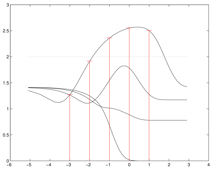
Figure 2: The expression (7) for lengths $0.03\leq l\leq 7.5$ and $r=0$, $0.5$, $1$, and $2$ from the lowest to the highest curve. The Bell inequality is violated whenever the value exceeds 2, e.g., when $l=1$ and $r=2$. The indicated values for $r=2$ will be used below.

Returning to position, write the measured position in base 2, e.g.,

$$Q=5.296875_{10}=101.0100110_{2},$$ (18)

which is an expression on the form

$$Q=\sum_{k=-\infty}^{\infty}2^{k}B_{k}.$$ (19)

Note that when the “zeroth” bit $B_{0}$ is 1, the corresponding measured value $S_{z,1}$ (i.e., $l=1$) would have been $-1$. Also when the zeroth bit $B_{0}$ is 0, the corresponding measured value $S_{z,1}$ would have been $+1$. We have $S_{z,1}=1-2B_{0}$, and in general

$$S_{z,2^{k}}=1-2B_{k}.$$ (20)

Multiplying two spin values corresponds to taking xor on the appropriate bit values (see Ref. Larsson (2003)), so that

$$SS^{\prime}=1-2B\overline{\lor}B^{\prime}$$ (21)

It is also simple to introduce a parameter $\phi$ so that

$$S_{\phi,2^{k}}=1-2B_{\phi,k}$$ (22)

Using this last correspondence and Eq. (21), the Bell inequality (5) becomes

$$\begin{split}&\big{|}E(B_{\alpha,k}\overline{\lor}B^{\prime}_{\gamma,k})+E(B_{\alpha,k}\overline{\lor}B^{\prime}_{\delta,k})-1\big{|}\\ &\quad+\big{|}E(B_{\beta,k}\overline{\lor}B^{\prime}_{\gamma,k})-E(B_{\beta,k}\overline{\lor}B^{\prime}_{\delta,k})\big{|}\leq 1.\end{split}$$ (23)

The right-hand side is a factor of two lower than before, but the sensitivity to noise and such-like is the same as before, we have just changed notation.

In our new notation, we can use the corresponding quantum expression to obtain a quantum bit (“qubit”)

$$s_{\phi,2^{k}}=1-2b_{\phi,k}$$ (24)

and a “quantum xor”

$$ss^{\prime}=1-2b\overline{\lor}b^{\prime}$$ (25)

which is a noncommutative operation when used on the same subsystem (see Ref. Larsson (2003)). We obtain a quantum expression corresponding to (7),

$$\begin{split}&\big{|}\langle b_{0,k}\overline{\lor}b^{\prime}_{\frac{\pi}{4},k}\rangle+\langle b_{0,k}\overline{\lor}b^{\prime}_{-\frac{\pi}{4},k}\rangle-1\big{|}\\ &\quad\quad+\big{|}\langle b_{\frac{\pi}{2},k}\overline{\lor}b^{\prime}_{\frac{\pi}{4},k}\rangle-\langle b_{\frac{\pi}{2},k}\overline{\lor}b^{\prime}_{-\frac{\pi}{4},k}\rangle\big{|}.\end{split}$$ (26)

In Fig. 2 (vertically scaled by the factor $\frac{1}{2}$) there is a simultaneous, separate violation for $r=2$, and $k=1$, $0$, and $-1$, while there is no violation for, e.g., $k=-2$ and $-3$.

We have used our continuous hierarchy of pseudo-spin systems indexed by the (real-valued) variable $l$, but only for values $l=2^{k}$. The reason is that, to talk about simultaneous violation, the pseudo-spin systems must commute with each other. The spin-operator $s_{z,l}$ trivially commutes with the spin operator $s_{z,cl}$ for any $c$, but it does not commute with $s_{x,cl}$ for all $c$s, for example when $c=1$. However, these two do commute in an important special case, when $c$ is an even number. This is because changes to the wave function caused by $s_{z,l}$ are wholly within each interval translated by, e.g., $s_{x,2ml}$, and the changes are the same within each such interval. It is possible to show that the whole pseudo-spin system for length $l$ commutes with that for length $2ml$. Thus, there is an infinite commuting hierarchy of spin systems,

$$\{s_{z,2^{k}l},s_{+,2^{k}l}=(s_{-,2^{k}l})^{{\dagger}}\}_{k\in\mathbb{Z}}.$$ (27)

The measured position $Q$ was expanded in base 2. The same can be done for the quantum operator

$$q=\sum_{k=-\infty}^{\infty}2^{k}b_{k}=\sum_{k=-\infty}^{\infty}2^{k}\frac{1-s_{z,2^{k}}}{2}.$$ (28)

Here it becomes really important that $s_{z,2^{k}}$ all commute. Since also $s_{x,2^{k}}$ all commute, and $s_{y,2^{k}}$ all commute for different $k$, it is meaningful to write, e.g.,

$$q_{x}=\sum_{k=-\infty}^{\infty}2^{k}b_{x,k}=\sum_{k=-\infty}^{\infty}2^{k}\frac{1-s_{x,2^{k}}}{2},$$ (29)

and similarly for $q_{y}$. These would be pseudo-positions obtained by qubit rotations of the original position operator $q$. To emphasize the presence of a pseudo-spin system in the ordinary position measurement, one could write $q_{z}=q$, but this will not be done below. The infinite expansions have their own, more mathematical problems which will not be discussed further here, note that violations only occur for finite $k$ for our continuous, localized $|\psi_{\text{NOPA}}\rangle$ state. Let us use the truncated expression

$$Q_{\phi,\text{\textvisiblespace}}=2B_{\phi_{1},1}+B_{\phi_{0},0}+\frac{B_{\phi_{-1},-1}}{2}+\frac{B_{\phi_{-2},-2}}{4}+\frac{B_{\phi_{-3},-3}}{8}.$$ (30)

By using ineq. (23) for each bit in the above expression, and letting $\overline{\lor}$ denote bitwise xor, we obtain ($2+1+\frac{1}{2}+\frac{1}{4}+\frac{1}{8}=3.875$)

$$\begin{split}&\big{|}E(Q_{\alpha,\text{\textvisiblespace}}\overline{\lor}Q^{\prime}_{\gamma,\text{\textvisiblespace}})+E(Q_{\alpha,\text{\textvisiblespace}}\overline{\lor}Q^{\prime}_{\delta,\text{\textvisiblespace}})-3.875\big{|}\\ &\quad+\big{|}E(Q_{\beta,\text{\textvisiblespace}}\overline{\lor}Q^{\prime}_{\gamma,\text{\textvisiblespace}})-E(Q_{\beta,\text{\textvisiblespace}}\overline{\lor}Q^{\prime}_{\delta,\text{\textvisiblespace}})\big{|}\leq 3.875.\end{split}$$ (31)

Reading off the quantum values in Fig. 2, we get

$$\begin{split}&\big{|}\langle q_{\text{\textvisiblespace}}\overline{\lor}q^{\prime}_{\frac{\pi}{4},\text{\textvisiblespace}}\rangle+\langle q_{\text{\textvisiblespace}}\overline{\lor}q^{\prime}_{-\frac{\pi}{4},\text{\textvisiblespace}}\rangle-3.875\big{|}\\ &\quad\quad+\big{|}\langle q_{\frac{\pi}{2},\text{\textvisiblespace}}\overline{\lor}q^{\prime}_{\frac{\pi}{4},\text{\textvisiblespace}}\rangle-\langle q_{\frac{\pi}{2},\text{\textvisiblespace}}\overline{\lor}q^{\prime}_{-\frac{\pi}{4},\text{\textvisiblespace}}\rangle\big{|}\\ &\quad\approx 2\times 1.25+1.28+\frac{1}{2}\times 1.18\\ &\quad\quad+\frac{1}{4}\times 0.96+\frac{1}{8}\times 0.64\approx 4.7>3.875.\end{split}$$ (32)

Here, the operator $q_{\text{\textvisiblespace}}$ is the usual position operator $q$, truncated to the bits in question. The truncation is done for several reasons. First and perhaps most important, it is not beneficial to include bits where there is no Bell violation, but it is possible to include such bits as seen above. Second, we would expect the measurement devices to be of finite size, so that there is a natural upper bound; note that finite size devices do not introduce any substantial error in the above reasoning, since the Gaussian is well localized.

Finally, the devices have finite resolution so there is a natural lower bound. On should perhaps remark that this is a question of resolution rather than accuracy. Low accuracy would yield bit-result 0 when there should have been a bit-result 1 and vice versa; there would have been more noise in the data. However, realization of the measurements corresponding to the operators defined here is a difficult issue. At present there is no implementation known to the author that would give the desired properties. Note that the qubits are in principle present in any position measurement; consequently they could be used in quantum information processing. This latter possibility in itself will perhaps provide a motive to realize this proposal, rather than the Bell violation. In any case, a full analysis of possible experimental errors is better postponed until an experimental procedure is known.

We have a Bell inequality where one of the operators correspond to position, and a violation from the NOPA state. When the squeezing increases, the violation of the inequality increases, and it is to be expected that infinite squeezing will give a maximal violation at each qubit of the position operator. This, in turn, means that the original EPR state (infinite squeezing) will violate the above inequalities maximally. Because of lack of space and the more mathematical nature of a proper statement of this, it will be deferred to a later publication.

One possible extension is to use qutrits (spin-1 correspondence) instead of qubits in the approach, or indeed so-called qu$N$its (spin-$(N-1)/2$ correspondence) for arbitrary $N$, together with an inequality more suited to such a situation Kaszlikowski et al. (2000); Collins et al. (2002); Chen et al. . There is also the question of what settings are the best to put in place of $\alpha$, $\beta$, $\gamma$, and $\delta$ at finite squeezing. The violation is not at its highest when using the settings from this paper, as this paper concentrates on the more conceptual issues. The maximum is probably best found by numerical optimization, given that we have numerical data only.

We have achieved what we set out to do. And the perhaps unsurprising conclusion is that the NOPA state cannot be described by a local realist model, despite having a strictly positive Wigner function. Note, however, that it was necessary to augment $q$ with operators not directly related to the momentum operator $p$. Nevertheless, this formulation is somewhat closer to the original EPR paper than the traditional Bell approach.