Testing quantum correlations with nuclear probes

Abstract

We investigated the feasibility of quantum-correlation measurements in nuclear physics experiments. In a first approach, we measured spin correlations of singlet-spin (${}^{1}S_{0}$) proton pairs, which were generated in ¹H(d,²He) and ¹²C(d,²He) nuclear charge-exchange reactions. The experiment was optimized for a clean preparation of the ²He singlet state and offered a $2\pi$ detection geometry for both protons in the exit channel. Our results confirm the effectiveness of the setup for theses studies, despite limitations of a small data sample recorded during the feasibility studies.

E-mail: wortche@kvi.nl

1 Introduction

Entanglement is believed to be a genuine resource for quantum computers and quantum communication technology. Entanglement shows up in composite quantum systems where the subsystems do not have pure states of their own. This is a strict quantum phenomenon with no classical analogue. Entangled states of joint systems are non-local, meaning that the outcome of measurements performed separately on each subsystem at space-like separation cannot be reproduced by local-hidden-variables (LHV) models. Such non-locality can be revealed by a violation of an inequality which any LHV model must satisfy. Such inequality is the Bell-type inequality [1]. Experimental tests of the Bell-type inequality have so far been limited to measurements with photons [2] rather than measurements with massive Fermions with only one exception: a proton-spin correlation measurement performed by Lamehi-Rachti and Mittig (LRM) about 30 years ago [3]. Note, that quantum non-contextuality has recently been tested with massive Fermions in single-neutron interferometry experiment by Hasegawa et al. [4]. However, it is well known that, if a theory is contextual, it is not necessarily non-local.

The advantage of using massive Fermions to test Bell-type inequalities is that the particles are well localized and the singlet state of the pair can be well defined by measuring the internal energy of the two-proton system. In this paper, we studied the feasibility of examining spin-correlation measurements of proton pairs in a ${}^{1}S_{0}$ intermediate state generated in ¹H($d,^{2}$He)n and ¹²C($d,^{2}$He)¹²B nuclear charge-exchange reactions. By selecting events on basis of the structure of the excited state in the remaining nucleus and on basis of the internal energy of the ²He system, we achieve a clean preparation of proton pairs under controlled conditions. Our analysis of the experimental results described below is compatible with the pioneering LRM experiment. However, our experimental setup, the experimental procedure and the data analysis improved significantly in comparison to the LRM experiment with respect to the following issues:

• control of higher order multipole contamination of the singlet state,

• control of the contamination due to randomly correlated pairs,

• causal separation of the proton pairs,

• no preferred quantization axis because of $2\pi$ detection geometry and

• record of complete event topology.

We will structure this paper as follows. In the following section we give a brief overview of the experimental arrangement and the data analysis, whereas special requirements and the feasibility of spin-correlation measurements are emphasized. For details of the experimental setup and the ²He analysis we refer to Ref. [5]. In section 3 we discuss details of the spin-correlation analysis and in section 4 our results are presented.

2 Experimental setup

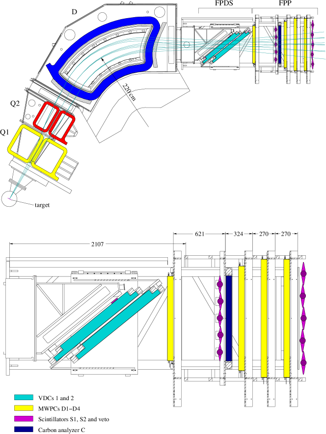
Figure 1: Schematic diagram of the experimental arrangement. Top part: The BBS spectrometer in conjunction with the ESN detector system. Lower part: Blown up view of the detector setup. The numbers indicate dimensions in units of mm. The focal-plane detection system (FPDS) is equipped with two VDCs to determine the four-momentum vectors of protons passing the spectrometer. Further downstream, the focal-plane polarimeter (FPP) set up, which consists of four MWPCs (D1, D2, D3, D4) and two plastic-scintillator arrrays (S1 and S2). A carbon analyzer (C) is placed just next to the scintillator S1.

The measurements were carried out using 172 MeV deuteron beams provided by the AGOR cyclotron of the Kernfysisch Versneller Instituut (KVI), Groningen. The deuterons were incident on a carbon foil of thickness 9.4 mg/cm², which was mounted in the scattering chamber of the Big-Bite Spectrometer (BBS) [6]. A schematic view of the experimental setup is shown in Fig. 1. The EuroSuperNova (ESN) detector system used consists of a pair of gas-filled Vertical-Drift Chambers (VDCs) for momentum reconstruction of the protons and a focal-plane polarimeter, which comprises Multi-Wire Proportional Chambers (MWPCs) and a pair of scintillator paddles S1 and S2 for time-of-flight and energy-loss measurements [5].

The ${}^{1}S_{0}$ proton pairs were prepared in a ¹²C(d,²He)¹²B nuclear charge-exchange reaction. A reaction of type (d,2p) is referred to as (d,²He) if the outgoing protons couple to the ${}^{1}S_{0}$ state. The ²He system is unbound by an internal energy of about 0.5 MeV, which is defined by the maximum of the (pp) ${}^{1}S_{0}$ final-state-interaction strength. The proton pairs emerging from the charge-exchange reaction were momentum analyzed in the BBS spectrometer, which was positioned at an angle $\theta_{BBS}=0^{\circ}$. The extreme forward angle was chosen to minimize the angular momentum transfer in the reaction which favors pure spin-flip (Gamow-Teller) type transitions and puts an additional constraint on the ${}^{1}S_{0}$ character of the proton pairs.

2.1 ²He identification

Due to the finite momentum and angular acceptances of the BBS focal plane, only proton pairs of relative kinetic energies less than 1 MeV in the ²He center of mass were detected as depicted in Fig. 2. The spectrometer therefore acted as a highly exclusive filter and contaminations of higher-order multipoles were limited to the percent level [7]. A dominant background of randomly correlated protons was due to the breakup of the deuteron, a reaction yielding protons with a momentum overlapping with the momentum range of interest. A clean identification of ²He events therefore necessitated a proper reconstruction of the excitation energy of the residual nucleus ¹²B and determination of the relative timing of the two correlated protons with a good resolution.

An event-trigger condition required that at least one proton passed through the spectrometer and was registered by coincident signals in scintillator planes S1 and S2. The coincidence window was set to less than 20 ns in order to minimize randoms caused by particles originating from different beam bursts each separated by 23 ns. The data, read out from the MWPCs, were fed into a fast online processing system, where they were tested on double-track conditions. Those events passing the test were stored for offline analysis.

Figure 2: Typical relative kinetic-energy distribution in the ²He center of mass obtained from the measured momenta of coincident protons.

The momentum vector and the focal-plane interception time of protons were determined in offline analysis [5] from the VDC data. After being triggered, the VDC TDC channels remained active for about 380 ns, which is the maximum drift-time associated with the events. A typical spectrum of the difference in focal-plane interception time corresponding to kinetic energies below the ¹²B $Q$-value is shown in the top left of Fig. 3. The ²He protons, which can for kinematical reasons be separated by at most a few $10^{-9}$ s (ns) in the BBS focal-plane, appear as a dominant prompt peak. The interception-time spectrum shows a peak centered at t=0 and satellite peaks due to random coincidences. The satellite peaks are due to randomly correlated proton pairs reflecting the beam-burst repetition rate. An effective identification of ²He events could be achieved by requiring an interception-time difference in the window $\pm$10 ns. An energy spectrum accumulated under this condition is shown in the lower right of Fig. 3. The kinetic energies were calculated for two-proton events assuming ²He kinematics [5]. The energy spectrum shows two prominent peaks superimposed on a continuous background (see top right of Fig. 3). The peak at 169 MeV corresponds to the $Q$-value of the ¹H(d,²He)n reaction and is due to a hydrogen contamination of the ¹²C target. The peak at 157 MeV corresponds to the $Q$-value ($Q=-14.81$ MeV) of the ¹²C(d,²He)¹²B reaction. The structures at lower kinetic energies correspond to transitions to ¹²B excited states. Unphysical energies larger than in the incident beam energy of 172 MeV are due to randomly correlated protons originating from the deuteron breakup. For the spin-correlation analysis, it was further required, that the sum of the kinetic energies of the proton pairs was equal to or less than the ¹²B threshold or in an energy window defined by the position and the width of the neutron peak.

Figure 3: Top left: Focal-plane interception-time difference for detected proton pairs. For the data set shown the random contamination is about 15%. Top right: Raw kinetic energy spectrum of detected proton pairs. Prominent peaks indicate ²He protons originating from the ¹²B ground-state transition and the p-n transition. Lower left: Kinetic energy spectrum gated on satellite peaks in the interception-time difference (no correlated protons). Lower right: Kinetic energy spectrum gated on the prompt peak in the interception-time difference.

3 Spin-correlation measurements and analysis

In order to measure the scattering angle in the carbon analyzer, identification of proton tracks upstream and downstream of the analyzer was required. We followed the fate of each proton [8] as it passed through the carbon analyzer, acquiring the information in the detector systems D1-D4 and S1, S2. We used only those events where both protons scattered into an angular range larger than 3 degrees in the carbon analyzer, since the most forward scattering is predominantly Coulomb type which is not spin dependent. The experimental setup provided the flexibility to arbitrarily choose the reference axis during the off-line analysis.

Figure 4: Geometry applied for extracting the experimental correlation function Eq. 3. The primary target is indicated by ¹²C, the primary scattering normal $\vec{n}_{\rm{}^{2}He}$ refers to the incoming deuteron and ²He center-of-mass movement, $\vec{y}$ is the normal to the BBS (horizontal) symmetry plane. The momenta of proton 1 and proton 2 upstream the analyzer are indicated by $\vec{p}_{1(2)}$, downstream the analyzer by $\vec{p}\,^{\prime}_{1(2)}$, and the normal and angle of the analyzing scattering for proton 1 (2) are indicated by $\vec{n}_{1(2)}$ and $\theta_{1(2)}$, respectively. The angle between the proton momenta $\vec{p}_{1(2)}$ is given by $\theta_{pp}$.

The correlation function $P(\theta)$ for two spin-${1\over 2}$ states can be measured according to

$$P(\theta)=\frac{N_{++}+N_{--}-N_{+-}-N_{-+}}{N_{++}+N_{--}+N_{+-}+N_{-+}}=\frac{N_{++}+N_{--}-N_{+-}-N_{-+}}{N_{total}}\,,$$ (1)

where $\theta$ is the angle between two arbitrary quantization directions $\vec{Q}_{1}$ and $\vec{Q}_{2}$ orthogonal to the momenta $\vec{p}_{1}$ and $\vec{p}_{2}$ of the two correlated protons, i.e. $\vec{Q}_{1}\perp\vec{p}_{1}$ and $\vec{Q}_{2}\perp\vec{p}_{2}$ and $N_{++}$ ($N_{--}$) is the number of events, where both protons scatter to the left (right) of the quantization direction and $N_{+-}$ $(N_{-+})$ is the number of events, where proton 1 scatters to the left (right) and proton 2 scatters to the right (left) and $N_{total}$ is the total number of events. Taking into account the finite analyzing power of the carbon analyzer, the number of events, in the above correlation function have to be weighted on an event-to-event basis by the analyzing powers $A^{1,2}_{y}(\theta_{1,2},E_{1,2})$ [9]

$$N^{w}_{++(--,+-,-+)}=\sum_{++(...)}\frac{1}{A^{1}_{y}(\theta_{1},E_{1})}\cdot\frac{1}{A^{2}_{y}(\theta_{2},E_{2})}$$ (2)

yielding the experimental correlation function $P_{exp}$ (see also LRM [3])

$$P_{exp}(\theta)=\frac{N_{++}^{w}+N_{--}^{w}-N_{+-}^{w}-N_{-+}^{w}}{N_{total}}\,.$$ (3)

The geometry applied to extract the experimental correlation function Eq. 3 is shown in Fig. 4 and Fig. 5. The correlation analysis was only applied for events where the direction of the primary scattering normal $\vec{n}_{i}$ deviated less than $1^{\circ}$ from the normal of the BBS symmetry plane $\vec{y}$. Due to this selection, our analysis became compatible with the LRM analysis [3].

The sign convention for the correlations is shown in Fig. 5, where the example of a right-right $(-\,-)$ correlation is depicted. The quantization axis $\vec{Q}_{1(2)}$ is chosen along the scattering normal $\vec{n}_{1(2)}$ with the convention, that the projection on the normal the BBS symmetry plane $\vec{Q}_{1(2)}\cdot\vec{y}$ is positive. According to this convention, a positive definite projection of the scattering normal $\vec{n}_{1(2)}\cdot\vec{y}$ indicates scattering to the left, a negative definite projection scattering to the right of the quantization axis.

The correlation angle $\theta$ (see Fig. 5) is defined as

$$\theta=|\varphi_{1}-\varphi_{2}|\,,$$ (4)

whereas the angle $\varphi_{1(2)}$ is measured in respect to the vector $\vec{x}_{1(2)}$ given by

$$\vec{x}_{1,2}=\vec{y}\times\vec{p}_{1(2)}\,.$$ (5)

The definition of $\varphi_{1(2)}$ and $\theta$ holds also for finite $\theta_{i}$ because of the purely transverse character of the analyzing reaction.

In quantum theory, the operator that corresponds to the correlation function is

$$P=\vec{Q}_{1}\cdot\vec{\sigma}\otimes\vec{Q}_{2}\cdot\vec{\sigma}\,,$$ (6)

acting in the Hilbert space ${{H_{\rm 1}}\otimes{H_{\rm 2}}}$ in $2\otimes 2$ dimension and $\vec{\sigma}$ are the Pauli matrices. The correlation function $P_{QM}$ is given by the mean value of this operator. For a pure state this correlation function could be easily computed. For a singlet state we have

$$P_{QM}^{\rm Singlet}(\theta)=-\cos\theta.$$ (7)

However, if the state is mixed the mean value should be averaged over the ensemble. Taking into account the effect of a random contamination of the pure singlet state, the quantum expectation deviates from Eq. 7. In fact, we introduce a factor $\gamma$ which interpolates between the unpolarized state $I/4$ and the singlet state $|\Psi^{-}\rangle=(|+-\rangle-|-+\rangle)/\sqrt{(}2)$, with $I$ the unit matrix.

Figure 5: Sign convention for the correlations depicted for a right-right $(-\,-)$ event and $\theta_{pp}=0^{\circ}$.

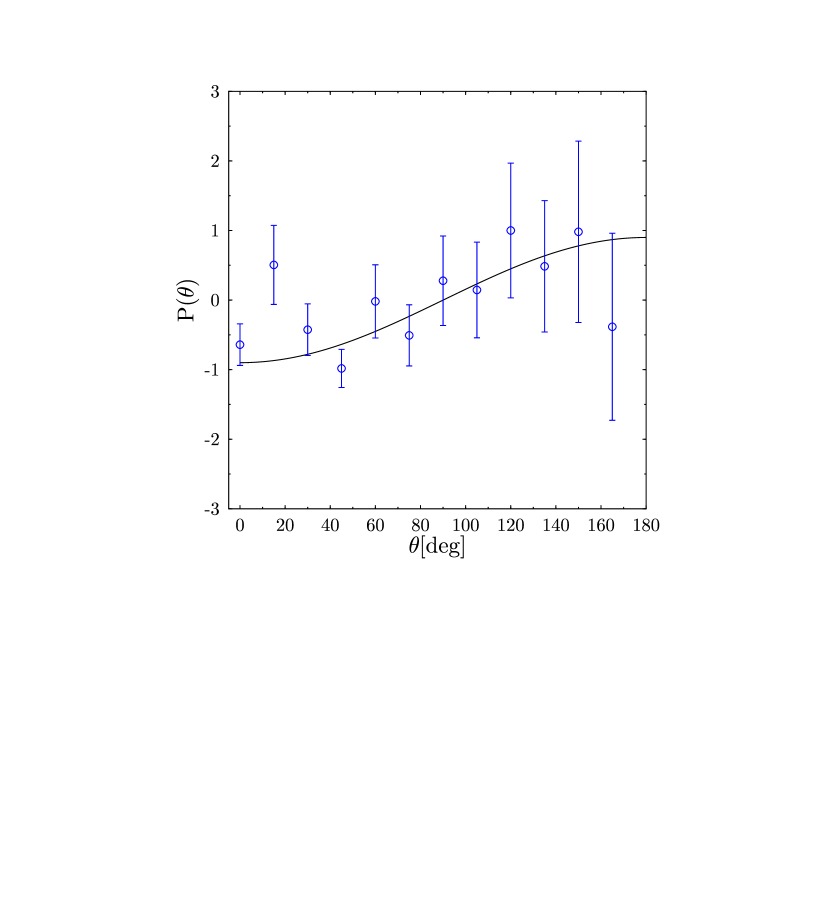
Figure 6: The extracted experimental correlation function $P_{exp}(\theta)$ (Eq. 3) in comparison with the quantum mechanics prediction $P_{QM}^{Werner}$ (Eq. 9) for $\gamma=0.9$

.

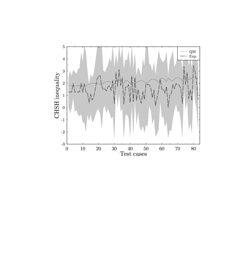
Figure 7: CHSH inequality for all possible combinations found from the probability shown in Fig. 6. The dashed line shows the experimental results, the dotted line the QM prediction. The shaded band represents the statistical error.

The density matrix of such a state is called Werner states [10] and it is given by

$$\rho_{W}=(1-\gamma){I\over 4}+\gamma|\Psi^{-}\rangle\langle\Psi^{-}|\,$$ (8)

This effect reduces the quantum expectation value of the correlation functions as follows

$$P_{QM}^{Werner}(\theta)=-\gamma\cos\theta\,.$$ (9)

4 Results

During two days of data taking, the mean rate of ²He events ending up in the correlation analysis amounted to about 0.1 Hz/nA, despite the fact that the (d,²He) production rate was nearly a factor 50 higher. This loss in statistics was mainly due to inefficiencies in the particle tracking downstream the analyzer. For the final analysis the data were binned into 12 angular $\theta$ bins, which yielded on average $10^{3}$ events per angle bin.

The random events, i.e. events shown in the lower left of Fig. 3, yielded an averaged correlation $\bar{P}_{exp}=0.05\pm 0.7$ per angle, which justifies the treatment of the background as a random contribution as indicated in Eq. 9. The overall mean of random events contributing to the prompt events amounted to 10%.

In Fig. 6 we show the extracted experimental correlation function $P_{exp}$ in comparison with the quantum mechanics prediction for Werner states Eq. 9 for $\gamma=0.9$. Despite of the large uncertainties the data exhibit a trend which agrees well with the quantum-mechanics prediction and yields a $\chi^{2}/{d.o.f}=\sum_{i}(P_{exp}^{i}-P_{QM}^{i})/\Delta P_{exp}^{i})^{2}=0.96$, which has to be compared with $\chi^{2}/{d.o.f}=1.93$ if $P_{QM}$ is replaced by $P_{const}=0$.

In order to demonstrate the power of the presented experimental approach, we further used the values we obtained for $P_{exp}$ to extract the values for a correlation function proposed by Clauser, Horne, Shimony and Holt (CHSH) [11] which can be written in the form

$$|P(\theta_{a},\theta_{b},\theta_{c})|=|P(\theta_{a})-P(\theta_{a}+\theta_{b})|+|P(\theta_{a}+\theta_{b}+\theta_{c})+P(\theta_{a}+\theta_{c})|\,,$$ (10)

with $\theta_{a,b,c}$ various sets of correlation angle $\theta$. All possible angular combinations yield 84 test cases which have been plotted in Fig. 7 in comparison with the quantum-mechanics predictions. A discussion of the CHSH-type correlations is beyond the scope of the present paper and will be the topic of a forthcoming publication [12]. From Fig. 7 it becomes obvious that the present experimental data set suffers from large statistical uncertainties. Nevertheless, the data exhibit a tendency to stay below the quantum mechanical results. A fact which would point towards classical scenarios.

5 Conclusion

In this paper, we presented a new experimental approach to study the feasibility of examining spin-correlations measurements in nuclear physics. With an improved detector setup, which removes the ambiguity in the track reconstruction, measurements with significant precision will become feasible. We are convinced that our experiments will have many potential applications in future quantum communication technology.

This work was performed as part of the research program of the Stichting voor Fundamenteel Onderzoek der Materie (FOM) with financial support from the Nederlandse Organisatie voor Wetenschappelijk Onderzoek . It was supported by the NSERC Canada, the European Union through the Human Capital and Mobility Program and the Fund for Scientific Research (FSR) Flanders.

References

- [1] J.S. Bell, Physics 1, 195 (1964); Rev. Mod. Phys. 38, 447 (1966).
- [2] A. Aspect, Nature 398, 189 (1999).
- [3] M. Lamehi-Rachti and W. Mittig, Phys. Rev. D 14, 2543 (1976).
- [4] Y. Hasegawa, R. Loidl, G. Badurek, M. Baron, and H. Rauch, Nature 425, 45 (2003).
- [5] S. Rakers, F. Ellinghaus, R. Bassini, C. Bäumer, A.M. van den Berg, D. Frekers, D. De Frenne, M. Hagemann, V.M. Hannen, M.N. Harakeh, M. Hartig, R. Henderson, J. Heyse, M.A. de Huu, E. Jacobs, M. Mielke, J.M. Schippers, R. Schmidt, S.Y. van der Werf, and H.J. Wörtche, Nucl. Instr. and Meth. 481, 253 (2002).
- [6] A.M. van den Berg, Nucl. Instr. Meth. B 99, 637 (1995).
- [7] S. Kox et al., Nucl. Phys. A 556, 621 (1993).
- [8] J. Heyse, Thesis, Universiteit Gent, 2002.
- [9] M.W. McNaughton, B.E. Bonner, H. Ohnuma, O.B. van Dijk, Sun Tsu-Hsun, C.L. Hollas, D.J. Gremans, K.H. McNaughton, P.J. Riley, R.F. Rodebauch, Shen-Wu Xu, S.E. Turpin, B. Aas, and G.S. Weston, Nucl. Instr. Meth. A 241, 435 (1985).
- [10] R.F. Werner, Phys. Rev. A 40, 4277 (1989).
- [11] J. Clauser, M. Horne, A. Shimony, and R. Holt, Phys. Rev. Lett. 23, 880 (1969).
- [12] C. Polachic, C. Rangacharyulu, A.M. van den Berg, S. Hamieh, M.N. Harakeh, M. Hunyadi, M.A. de Huu, H.J. Wörtche, J. Heyse, C. Bäumer, D. Frekers, J.A. Brooke, and P. Busch, submitted to Phys. Lett. A.