Quantum state targeting

Abstract

We introduce a new primitive for quantum communication that we term “state targeting” wherein the goal is to pass a test for a target state even though the system upon which the test is performed is submitted prior to learning the target state’s identity. Success in state targeting can be described as having some control over the outcome of the test. We show that increasing one’s control above a minimum amount implies an unavoidable increase in the probability of failing the test. This is analogous to the unavoidable disturbance to a quantum state that results from gaining information about its identity, and can be shown to be a purely quantum effect. We provide some applications of the results to the security analysis of cryptographic tasks implemented between remote antagonistic parties. Although we focus on weak coin flipping, the results are significant for other two-party protocols, such as strong coin flipping, partially binding and concealing bit commitment, and bit escrow. Furthermore, the results have significance not only for the traditional notion of security in cryptography, that of restricting a cheater’s ability to bias the outcome of the protocol, but also on a novel notion of security that arises only in the quantum context, that of cheat-sensitivity. Finally, our analysis of state targeting leads to some interesting secondary results, for instance, a generalization of Uhlmann’s theorem and an operational interpretation of the fidelity between two mixed states.

I Introduction

It is well known that quantum theory allows for the implementation of cryptographic tasks with a degree of information-theoretic security that cannot be achieved classically, with key distribution being the most famous example BB84 . Particularly interesting among these tasks are the so-called “post-cold-war” applications of cryptography, wherein two remote and mistrustful parties seek to cooperate towards some end. Examples of these are bit commitment Mayers ; LoChau ; SpekkensRudolphBC , strong coin flipping Aharonov ; Ambainis , weak coin flipping wcf , bit escrow Aharonov , and two-party secure computation Lo . In this paper, we focus on elucidating a certain primitive we have identified as accounting for the ability of certain quantum two-party cryptographic protocols to outperform their classical counterparts.

We begin by recalling a more familiar such primitive, specifically state estimation helstrom : A system is prepared in one of a set of states, and passed on to an estimator. Typically, the task of the estimator is to try, as best as possible, to determine which of the states describes the system. Imagine, however, that the estimator is asked to announce his guess of the state and then is asked to resubmit the system, which is subsequently subjected to a pass/fail test for still being in the initially prepared state. In this case, the estimator’s task is to guess the state without disturbing it. By doing nothing to the system, the estimator can make a random guess and avoid creating any disturbance. However, it is well known that any interaction with the system that leads to a greater probability of guessing correctly will necessarily also lead to a disturbance of the state fuchs . This phenomena is extremely important - for instance, it underlies the possibility of quantum key distribution.

The focus of this paper is the task of passing a test for a target state, even though the system upon which the test is performed must be submitted prior to learning the target state’s identity. We call this task state targeting. State targeting is built of the same elements as the sort of state estimation task just discussed: There is a system and a set of states, one of which is distinguished. There is also a classical announcement of a state drawn from the specified set, and the most desirable announcement is an announcement of the distinguished state. Finally, there is a pass/fail test on the system. What is different in state targeting is how these elements are organized, and the fact that the person implementing the task (the player) submits rather than receives the quantum system.

More explicitly, a state targeting task proceeds as follows. At the outset, there is an unknown target state, drawn from a known set of states. The player submits a system, and only after doing so does she learn the identity of the target state. At this point, the player must announce a state from the original set (not necessarily the target state), and the system is subjected to a pass/fail test for the announced state. Success is defined as announcing the target state and subsequently passing the test for this state.

The player can always make a random guess of the target state initially, and thereafter announce this state and be sure to pass the test for this state. This will lead to some finite probability of announcing the target state while avoiding any risk of failing the final test. However, it turns out that any attempt to make the probability of announcing the target state greater than what is achieved with this trivial scheme results in a non-zero probability of failing the final test. This phenomena is analogous to the unavoidable disturbance that comes with information gain in state estimation. As one might expect, it too has interesting applications in quantum cryptography.

The outline of the paper is as follows. In section II, we provide a simple cryptographic motivation for our study, namely, a weak coin flipping(WCF) protocol wherein one of the party’s cheating strategies is an instance of state targeting. We also define the task of state targeting in greater detail than has been done in the introduction. In section III, we consider state targeting where the target state is drawn uniformly from a pair of pure states. We determine the maximum probability of success, and investigate the rate at which the probability of failing the final test increases with the probability of success. Section IV generalizes the notion of state targeting by allowing for the possibility that the player simply declines from announcing a state. This allows the player to achieve some non-trivial degree of success without running any risk of failing the final test. (This is analogous to the fact that some information gain without disturbance becomes possible in state estimation if one has the option to sometimes decline from resubmitting the system for testing.) This variant of the state targeting task is also shown to have a cryptographic motivation in terms of a weak coin flipping protocol. In section V, we optimize this variant in the case where the target state is drawn uniformly from a pair of pure states.

In the second half of the paper, we consider state targeting for mixed states. This requires a careful consideration of what to use as a test for a mixed state, and so we begin in section VI by addressing this question. In section VII, we consider the success that can be achieved in state targeting between a pair of mixed states, and in section VIII, we examine the case where the player is allowed to sometimes decline from being tested. Section IX refines the analogy that exists between state targeting and state estimation by focusing on a variant of state estimation, which we call state spying, wherein the estimator must resubmit the system for testing. We consider the applications of our results on state targeting and discuss some open problems in section IX. Finally, in section X, we consider the classical analogue of state targeting, which highlights the inherently quantum mechanical features of this task.

II Motivation and definition of state targeting

To emphasize the importance of state targeting in cryptography, and to motivate the sorts of problems that we shall address, it is useful to have an example of a protocol that makes use of this task. For this purpose, we introduce a very simple protocol for the two-party cryptographic primitive of weak coin flipping(WCF) wcf wcf . Here, two separated and mistrustful parties wish to engage in communication to generate a random bit, the value of which will fix a winner and a loser, in such a way that each party can be guaranteed that if they follow the honest protocol, the other party is limited in the extent to which they can bias the value of the bit in their favor.

The simple weak coin flipping protocol we consider makes use of a pair of non-orthogonal pure states $|\psi_{0}\rangle$,$|\psi_{1}\rangle$. If both parties are honest, it proceeds as follows.

Weak coin flipping protocol 1

• Alice chooses a bit $b$ uniformly from {0,1}, prepares $|\psi_{b}\rangle$ and sends the system to Bob.

• Bob chooses a bit $b^{\prime}$ uniformly from {0,1} and announces it to Alice (one can think of this as Bob’s guess of the value of $b$).

• Alice announces $b$ to Bob

• Bob tests the system for being in the state $|\psi_{b}\rangle$.

  If at step (4), the system fails Bob’s test, then Alice is caught cheating. Otherwise, if $b^{\prime}=b$ then Bob wins, while if $b^{\prime}\neq b$, then Alice wins.

Alice may cheat by preparing the system in an arbitrary state of her choosing at step (1), and making whatever announcement she pleases at step (3). Bob may cheat at step (2) by performing a measurement upon the system, and using the outcome to inform his decision of what $b^{\prime}$ to announce. The extent to which Bob can cheat when Alice is honest depends on the extent to which he can correctly estimate which of a pair of non-orthogonal states applies to the system, in order to make the best possible guess of $b$ and maximize his probability of making $b^{\prime}=b$. The problem of state estimation has been extensively studied, and consequently the solution can be found in the literature helstrom ; fuchs . On the other hand, the extent to which Alice can cheat when Bob is honest depends on the extent to which she can pass a test for the state opposite to the one Bob guessed, despite not knowing what Bob’s guess will be when she submits the system. We can state this as follows: her target state is determined by Bob’s announcement, which only occurs after she has submitted the system. This is a simple instance of state targeting.

Note that Alice’s announcement in step (3) of the protocol determines what state Bob is to test for. Alice can only win the coin flip if she announces a bit $b$ that is unequal to $b^{\prime}$. However, if she announces $b\neq b^{\prime}$ without having initially prepared $|\psi_{b}\rangle$, then she runs a risk of failing Bob’s test. Of course, Alice may sometimes prefer to pass a test for the non-target state rather than failing the test for the target state. As such, she may not always ask Bob to test for the target state.

The task faced by a dishonest Alice in our simple WCF protocol is just one instance of state targeting. More generally, a state targeting task is defined as follows:

• Alice submits a system to Bob.

• Alice learns the identity of the target state.

• Alice announces a state to Bob (not necessarily the target state).

• Bob performs a Pass/Fail test for the announced state.

The possible outcomes are:

• Alice announces the target state and passes Bob’s test

• Alice announces the target state and fails Bob’s test

• Alice announces a non-target state and passes Bob’s test

• Alice announces a non-target state and fails Bob’s test

“Success” in state targeting is to achieve outcome (A). Thus, we can quantify the degree of success by the probability of this outcome. We call this probability Alice’s control We shall be interested in determining the maximum control achievable in state targeting.

There are several ways in which Alice might not succeed. In cryptographic applications, it is reasonable to expect that failing one of Bob’s tests has a greater cost than passing the test for a non-target state, since the former indicates that Alice has cheated. Thus, it is useful to consider the total probability of failing Bob’s test, which is the sum of the probabilities for outcomes (B) and (D). We call this probability Alice’s disturbance. It is sometimes useful for Alice to sacrifice some control to lower her disturbance. Thus, we shall be interested in determining the minimal disturbance for a given control, which we refer to as the optimal control-disturbance trade-off.

III State targeting for two pure states

III.1 Maximum control

Consider the example of state targeting that is provided by our simple weak coin flipping protocol, namely, one wherein the target is selected uniformly from a pair of pure states, $|\psi_{0}\rangle,|\psi_{1}\rangle$. If Alice simply wishes to maximize her probability of announcing the target state and passing Bob’s test, that is, if she is unconcerned about the relative probabilities of outcomes (B),(C) and (D), then she should always announce the target state. Her most general strategy at step (i) is to prepare the system in a (possibly mixed) state $\rho$. In this case, Alice’s control is

$$C=\frac{1}{2}\langle\psi_{0}|\rho|\psi_{0}\rangle+\frac{1}{2}\langle\psi_{1}|\rho|\psi_{1}\rangle.$$ (1)

Noting that this can be rewritten as $\frac{1}{2}{\rm Tr}(\rho(|\psi_{0}\rangle\langle\psi_{0}|+|\psi_{1}\rangle\langle\psi_{1}|)$, it is clear that the maximum control is simply the maximum eigenvalue of $|\psi_{0}\rangle\langle\psi_{0}|+|\psi_{1}\rangle\langle\psi_{1}|$ and is achieved by choosing $\rho$ to be the associated eigenvector. Explicitly, the maximum control is

$$C^{\max}\equiv\max_{\rho}\,C=\frac{1}{2}(1+|\langle\psi_{0}|\psi_{1}\rangle|)$$ (2)

and the state that achieves it is

$$|\psi_{M}\rangle\equiv{\cal N}(|\psi_{0}\rangle+|\psi_{1}\rangle),$$ (3)

where ${\cal N}$ is a normalization factor, and the phases have been chosen so that $\langle\psi_{0}|\psi_{1}\rangle$ is real.

Since the Hilbert space spanned by any pair of pure states is two-dimensional, it can be represented using the Bloch sphere picture. Within this picture, $|\psi_{M}\rangle$ is represented by the point that lies halfway between the points representing $|\psi_{0}\rangle$ and $|\psi_{1}\rangle$ on the geodesic that connects them, as indicated in Fig. 1.

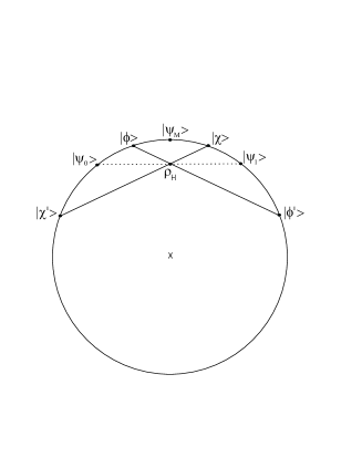
Figure 1: A slice of the Bloch sphere, showing the two possible target states, $|\psi_{0}\rangle$ and $|\psi_{1}\rangle$. The state $|\psi_{M}\rangle$ is the one that Alice must submit to achieve her maximal control. If she submits the state $\rho_{H}$, then she can achieve some non-trivial control at the cost of some disturbance by steering to a particular convex decomposition of the state prior to her announcement. The pair of states $|\phi\rangle,|\phi^{\prime}\rangle$ indicate the elements of a convex decomposition that Alice might use where the target state is $|\psi_{0}\rangle$. In general the optimal state to submit in order to minimize her disturbance for a given control lies between $\rho_{H}$ and $|\psi_{M}\rangle$.

III.2 The control-disturbance trade-off

By achieving her maximum control, Alice runs a risk of failing Bob’s test. Since she always announces the target state in this case, outcomes (C) and (D) never occur and her probability of failing Bob’s test (her disturbance) is simply the difference between 1 and her maximum control, that is, $\frac{1}{2}(1-|\langle\psi_{0}|\psi_{1}\rangle|)$. If, on the other hand, Alice exerts her trivial control of 1/2 by preparing $|\psi_{0}\rangle$ or $|\psi_{1}\rangle$ with equal probability and then announcing this state regardless of the identity of the target state, she creates no disturbance. We can imagine, however, that situations may arise wherein Alice decides to achieve some non-trivial but non-maximal control. It is useful therefore to determine the minimal disturbance for every achievable degree of control. Since we find that this function is monotonically increasing, it also specifies the maximum control for a given disturbance.

We begin by making the observation that a second strategy for Alice which achieves the trivial control with no disturbance is for her to couple the system she sends to Bob with an ancilla that she keeps, thereby preparing the entangled state

$$\frac{1}{\sqrt{2}}\left(|0\rangle|\psi_{0}\rangle+|1\rangle|\psi_{1}\rangle\right).$$ (4)

When it comes time to announce a state to Bob, she simply measures the ancilla in the $|0\rangle,|1\rangle$ basis, registers the bit value $b$ of the outcome, and announces $|\psi_{b}\rangle$.

In this situation the reduced density operator for the submitted system is $\rho_{H}=\frac{1}{2}|\psi_{0}\rangle\langle\psi_{0}|+\frac{1}{2}|\psi_{1}\rangle\langle\psi_{1}|$, which is represented on the Bloch sphere by the point which lies halfway along the line joining the points corresponding to $|\psi_{0}\rangle$ and $|\psi_{1}\rangle$ - this is depicted in Fig. 1.

Alice can now use the following trick to increase her control beyond the minimum value. Suppose Bob announces that the target state is $|\psi_{0}\rangle$. Alice then implements a measurement on her ancilla of some basis distinct from the ${|0\rangle,|1\rangle}$ basis. This collapses the state of the submitted system to $|\phi\rangle$ with some probability $q$ and to $|\phi^{\prime}\rangle$ with probability $(1-q$). An example is depicted in Fig. 1. We assume that of the two states, $|\phi\rangle$ has the greater overlap with $|\psi_{0}\rangle$ (as is the case in the figure), so that Alice announces $|\psi_{0}\rangle$ upon obtaining the outcome associated with $|\phi\rangle$, and she announces $|\psi_{1}\rangle$ upon obtaining the outcome associated with $|\phi^{\prime}\rangle$. If the target state is $|\psi_{1}\rangle$, she exerts a similar strategy, collapsing the state of the submitted system to a different pair of states, $|\chi\rangle$ or $|\chi^{\prime}\rangle$, with probabilities $p$ and $1-p$ respectively.

By this strategy, Alice achieves a control of

$$C=\frac{1}{2}q|\langle\phi|\psi_{0}\rangle|^{2}+\frac{1}{2}p|\langle\chi|\psi_{1}\rangle|^{2}.$$ (5)

Her disturbance, which is her total probability of failing Bob’s test, is

$$D = \frac{1}{2}[q(1-|\langle\phi|\psi_{0}\rangle|^{2})+(1-q)(1-|\langle\phi^{\prime}|\psi_{1}\rangle|^{2}]$$ (6)

$$+ \frac{1}{2}[p(1-|\langle\chi|\psi_{1}\rangle|^{2})+(1-p)(1-|\langle\chi^{\prime}|\psi_{0}\rangle|^{2}]$$

One might worry that of all the convex decompositions of $\rho_{H}$, only some can be realized by performing a measurement on the ancilla. If this were the case, then this subset of convex decompositions would have to be characterized before we could proceed with the optimization. However, this is not a concern, because as is shown in Refs. schr32 and HJW (and generalized to non-extremal decompositions in RudolphSpekkensQIC ), every convex decompositions of a mixed state can be achieved by some measurement on the ancilla. Thus, we can vary over all convex decompositions with the assurance that there is a measurement that will achieve it. Assuming $|\psi_{0}\rangle$ and $|\psi_{1}\rangle$ are non-orthogonal, $\rho_{H}$ lies off the centre of the Bloch sphere, and consequently $|\phi\rangle$ and $|\phi^{\prime}\rangle$ (which define the convex decomposition of $\rho_{H}$) can be chosen such that $q>1/2$; this follows from the fact that $\rho_{H}$ is geometrically closer to $|\phi\rangle$ than to $|\phi^{\prime}\rangle$ in the Bloch sphere. Similarly, Alice can ensure that $p>1/2$. Despite the fact that Alice has a non-unit probability of passing Bob’s test, her overall probability of success can increase.

Figure 2: The control disturbance tradeoff for two pure states, with $|\langle\psi_{0}|\psi_{1}\rangle|^{2}=1/2$. Curve (a) is for the case where Alice does not have the option to decline from being tested, considered in section III.2, whereas curve (b) is for the case where she does, considered in section V.2. For the former, the disturbance is non-zero for every control above 1/2, while for the latter it is only non-zero after the point indicated in the diagram.

We do not expect that $\rho_{H}$ will correspond to the optimal $\rho$ for every value of the control that Alice may wish to achieve. Indeed, we already know that in order to achieve her maximum control, she must submit a different state, indicated by $|\psi_{M}\rangle$ in Fig. 1. Thus we expect the optimal $\rho$ to be an interpolation between $\rho_{H}$ and $|\psi_{M}\rangle$ as we increase $C$ from $1/2$ to $C^{\max}$. So, we must perform two optimizations: an optimization over the state $\rho$ of the submitted system, and an optimization over the convex decomposition of $\rho$ she should realize prior to announcing to Bob which state he should test for.

It is not difficult to show that the optimal $\rho$ has a Bloch vector that bisects the Bloch vectors representing $|\psi_{0}\rangle$ and $|\psi_{1}\rangle$, and that the optimal convex decomposition to realize when $|\psi_{1}\rangle$ is the target state is simply the mirror image in the Bloch sphere of the optimal convex decomposition when $|\psi_{0}\rangle$ is the target state, so that $q=p$. These simplifications leave us with a two parameter optimization problem: the one parameter corresponding to the length $r$ of the Bloch vector representing $\rho$, the other parameter corresponding to the angle between the Bloch vectors representing $|\psi_{0}\rangle$ and $|\phi\rangle$. Although, we have not been able to perform this optimization analytically for very value of $|\langle\psi_{0}|\psi_{1}\rangle|$. The curve (a) in Fig. 2 depicts the optimal tradeoff for $|\langle\psi_{0}|\psi_{1}\rangle|^{2}=1/2$.

IV Motivation and definition of disturbance-free state targeting

In the context of the WCF protocol presented earlier, it may sometimes be the case that the consequences for Alice if she is caught cheating are sufficiently dire that she wishes to avoid this outcome at all costs. The question then becomes whether this is enough to guarantee that she follow the honest protocol. For the case of two non-orthogonal target states, if Alice submits some state distinct from one of these possibilities, then regardless of what she announces, she has a non-zero probability of failing Bob’s test. The only way to be certain to pass Bob’s test is to submit one of these states and to announce the same state, that is, to follow the honest protocol and achieve the trivial control of 1/2. This is reflected in curve (a) of Fig. (2) by the fact that for every value of control greater than 1/2 the disturbance is non-zero.

Nonetheless, there are useful versions of the task of state targeting wherein Alice has the option of declining from announcing a state to Bob, and in such cases, Alice can achieve greater than the trivial control without incurring any disturbance.

We again introduce a simple WCF protocol as motivation. This differs from the previous one in that both Alice and Bob are tested for cheating, which results in a protocol that offers fewer cheating possibilities for Bob, but more for Alice. If both parties are honest, the protocol proceeds as follows.

Weak coin flipping protocol 2

• Alice chooses a bit $b$ uniformly from {0,1}, prepares $|\psi_{b}\rangle$ and sends the system to Bob.

• Bob chooses a bit $b^{\prime}$ uniformly from 0,1 and announces it to Alice (one can think of this as Bob’s guess of which state Alice submitted).

• Alice announces $b$ to Bob

  If $b^{\prime}=b$, then

• Bob returns the system to Alice, and Alice tests the system for being in the state $|\psi_{b}\rangle$.

  Else, if $b^{\prime}\neq b$, then

• Bob tests the system for being in the state $|\psi_{b}\rangle$.

  If at step (4) the system fails Alice’s(Bob’s) test, then Bob(Alice) is caught cheating. Otherwise, if $b^{\prime}=b$ then Bob wins, while if $b^{\prime}\neq b$, then Alice wins.

As before, Alice may cheat by preparing the system in an arbitrary state of her choosing, and making whatever announcement she pleases. The difference is that if she announces $b^{\prime}=b$, then she is not tested by Bob.

This suggests a more general type of state targeting task, which differs from the one outlined in section II insofar as step (iii) is replaced by:

• Alice has the option of either (a) announcing a state to Bob (not necessarily the target state), or (b) declining to announce a state to Bob.

There is also an additional possible outcome relative to the version from the last section, namely:

• Alice declines to announce a state to Bob.

Because of this additional outcome, Alice can make her disturbance strictly zero while still achieving a non-trivial control. We call this disturbance-free state targeting. The control that Alice achieves by implementing her best disturbance-free state targeting is still defined as her probability of achieving outcome (A). We call this her disturbance-free control, and denote it by $C_{\textrm{df}}$. (An analogous quantity is defined in Ref. wcf , where it is called Alice’s threshold for cheat-sensitivity.)

The possibility of disturbance-free state targeting is analogous to something that occurs in unambiguous discrimination of pure statesIDP . (The latter is a procedure which either discriminates the states without any probability of error, or else simply returns the result “inconclusive”.) If the inconclusive outcome is not obtained, then the pure state with which the system was prepared is known with certainty, and can be re-prepared, so that a test for the initial state can be passed with certainty. If the inconclusive result is obtained, then the estimator declines from having the system tested. Thus, the existence of an inconclusive outcome allows for the possibility of information gain without disturbance. Analogously, the option to decline from being tested allows for non-trivial control without disturbance.

V Disturbance-free state targeting for two pure states

V.1 Maximum disturbance-free control

We now demonstrate how disturbance-free state targeting is achieved in the case where the target state is chosen uniformly from two non-orthogonal pure states. The technique is similar to the one used to minimize the disturbance for a given control. Alice initially couples the submitted system to an ancilla (which she keeps) so that the state of the pair is entangled. After learning the identity of the target state, she measures her ancilla in such a way that the state of the submitted system is updated according to a convex decomposition that contains the target state. If it happens to collapse to the target state, then she announces the target state, and is certain to pass Bob’s test. If it collapses to another state, then she simply declines to announce a state to Bob.

The fact that such a scheme can achieve a control greater than 1/2 can be seen by considering Fig. (3). If the state $\rho$ that Alice submits falls between $\rho_{H}$ and the completely mixed state (the centre of the Bloch sphere), and she steers to a two-element convex decomposition containing the target state, then because $\rho$ is necessarily geometrically closer to the target state than to the other element of the decomposition, and because greater geometric proximity represents a greater probability of collapsing to that element RudolphSpekkensQIC , it follows that the probability of announcing the target state is necessarily greater than 1/2.

We now proceed to find the maximum probability of disturbance-free state targeting. We must vary over both the convex decompositions for a fixed submitted state, and over the submitted states.

In the first optimization, we seek to find the largest probability with which the target state appears in a convex decomposition of the submitted state. A corollary we prove in section (VIII) establishes that the maximum probability of collapsing the state $\rho$ to the state $|\psi\rangle$ is

$$\frac{1}{\left\langle\psi\right|\rho^{-1}\left|\psi\right\rangle}.$$ (7)

Given that the target state is equally likely to be $|\psi_{0}\rangle$ or $|\psi_{1}\rangle$, the disturbance-free control for a submitted state $\rho$ is

$$C_{\text{df}}=\frac{1}{2}\frac{1}{\left\langle\psi_{0}\right|\rho^{-1}\left|\psi_{0}\right\rangle}+\frac{1}{2}\frac{1}{\left\langle\psi_{1}\right|\rho^{-1}\left|\psi_{1}\right\rangle}$$ (8)

We can now consider the optimization over $\rho$. Since there is clearly no advantage to preparing a $\rho$ outside of the subspace spanned by $\left|\psi_{0}\right\rangle$ and $\left|\psi_{1}\right\rangle,$ the problem can be entirely formulated in a two-dimensional Hilbert space, so that we may use the Bloch sphere representation of states. The optimization is done in Appendix A. The maximum disturbance-free control is found to be

$$C^{\text{max}}_{\text{df}}\equiv\max_{\rho}C_{\text{df}}=\frac{1}{1+\sqrt{1-\left|\left\langle\psi_{0}|\psi_{1}\right\rangle\right|^{2}}}.$$ (9)

The strategy that achieves this control requires Alice to prepare a mixed state of the form

$$\rho^{\mathrm{opt}}=\frac{\alpha}{2}I+\frac{1-\alpha}{2}\left(\left|\psi_{0}\right\rangle\left\langle\psi_{0}\right|+\left|\psi_{1}\right\rangle\left\langle\psi_{1}\right|\right),$$ (10)

where

$$\alpha=1-\frac{1}{2}\frac{1}{\left|\left\langle\psi_{0}|\psi_{1}\right\rangle\right|^{3}}\left(1-\sqrt{1-\left|\left\langle\psi_{0}|\psi_{1}\right\rangle\right|^{2}}\right).$$ (11)

It is easy to see that the maximum disturbance-free control, Eq. (9), is less than the maximum control, Eq. (2), for any pair of states. Thus, to avoid creating a disturbance, Alice must pay a price in control.

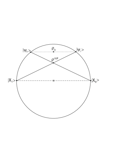
Figure 3: A section of the Bloch sphere showing the state $\rho^{\mathrm{opt}}$ that yields the largest disturbance-free control when the possible target states are $|\psi_{0}\rangle$ and $|\psi_{1}\rangle$.

In terms of the Bloch sphere picture, $\rho^{\mathrm{opt}}$ has a particularly simple geometric relation to $\left|\psi_{0}\right\rangle$ and $\left|\psi_{1}\right\rangle$, as is depicted in Fig. 3. Note that the states $|X_{0}\rangle$ and $|X_{1}\rangle$ are orthogonal and symmetric about $|\psi_{0}\rangle$ and $|\psi_{1}\rangle$. If the target state is $|\psi_{0}\rangle$, then Alice steers to the decomposition of $\rho^{\mathrm{opt}}$ containing $|\psi_{0}\rangle$ and $|X_{0}\rangle$.

V.2 The control-disturbance trade-off for state targeting with an option to decline

It is interesting to determine the minimal disturbance for a given control when there is an option to decline from announcing a state. In this case, the disturbance will be non-zero only for controls greater than the disturbance-free control. However, the disturbance for the maximal control is the same, since to achieve her maximal control, Alice must always announce the target state, and consequently never exercises her option to decline from announcing a state.

We consider this tradeoff in the simple case of two pure states. Suppose that Alice has submitted some $\rho$ and now learns that the target state is $|\psi_{0}\rangle$. As described in section III.2, she can make a measurement on the ancilla which collapses the submitted system to either the state $|\phi\rangle$ (with probability $q$) or to state $|\phi^{\prime}\rangle$ (with probability $1-q$). As before, if she collapses to the state $|\phi\rangle$ then she announces the state $|\psi_{0}\rangle$. Unlike before however, if she collapses $\rho$ to $|\phi^{\prime}\rangle$ then she declines to announce a state to Bob rather than announcing $|\psi_{1}\rangle$. A similar strategy is adopted if the target state is $|\psi_{1}\rangle$. This scenario does not affect the expression for the control that Alice achieves, it is still given by (5). However her disturbance is now given by

$$D=\frac{1}{2}q(1-|\langle\phi|\psi_{0}\rangle|^{2})+\frac{1}{2}p(1-|\langle\chi|\psi_{1}\rangle|^{2})$$ (12)

Once again the problem of minimizing Alice’s disturbance for a given control can be simplified to an optimization over only two parameters. The solutions to this optimization problem can be found analytically. Specifically, we obtain the optimal control and disturbance as parametric equations in a parameter $\mu$ which runs from 0 to $\theta$, where $\theta=|\langle\psi_{0}|\psi_{1}\rangle|$ by definition. Explicitly:

$$C^{opt} = \frac{1}{2}\frac{\cos\mu-\sin(\theta-\mu)}{1+\sin(\theta-\mu)}$$ (13)

$$D^{opt} = \frac{1}{2}\frac{1-\cos\mu}{1+\sin(\theta-\mu)}$$ (14)

The length $r$ of the Bloch vector corresponding to the optimal $\rho$ that Alice should submit for a given control is

$$r^{opt}=\frac{1-\sin(\theta-\mu)}{\cos(\theta-\mu)}$$ (15)

Curve (b) of Fig. (2) is a plot of this optimal tradeoff for $\theta=\pi/4$.

VI Testing for a mixed state

We have thus far examined state targeting under the assumption that the possible target states are pure. A useful and powerful generalization of state targeting occurs if we admit the possibility of mixed target states. Recall that the task of state targeting requires Bob to test the submitted system for being in the state announced by Alice. Thus, we must begin by discussing the possible ways in which one can test for a mixed state. Because greater difficulty in passing a test typically yields greater security for the protocol making use of it, we seek to find the tests that are most difficult to pass.

For convenience, we call the tester Bob and the one being tested Alice. The only kind of measurement on the submitted system alone that is always passed when the system is in the state $\sigma$ is one that is associated with a projector onto a subspace that is greater than or equal to the support of $\sigma.$ The most difficult such measurement to pass is the one associated with the projector onto the support of $\sigma$. We call this the support test for $\sigma$. Unfortunately, there are many other mixed states which always yield a positive outcome for this test, namely those having the same support as $\sigma.$ Thus, this test is relatively easy to pass.

Another interesting test is one that makes use of a particular convex decomposition of $\sigma$, that is, a set $\{p_{k},|\psi_{k}\rangle\}$ such that $\sum_{k}p_{k}|\psi_{k}\rangle\langle\psi_{k}|=\sigma$. The idea is that if Alice prepared the system in a state by drawing it from the set $\{|\psi_{k}\rangle\}$ according to the distribution ${p_{k}}$, then from Bob’s perspective, she has submitted the state $\sigma$. If Alice does not implement such a preparation, then it is possible for Bob to sometimes detect this fact; he simply demands that Alice announce the value of $k$ to him, and he then tests the system for being in the state $|\psi_{k}\rangle$. We call this a convex decomposition test for $\sigma$. This test is better than the support test, because if Alice initially prepares a mixed state that merely has the same support as $\sigma$, this does not guarantee that she can pass a convex decomposition test with certainty. Nonetheless, it is still a weak test since there any mixed states besides $\sigma$ that can pass the test with certainly, namely, any state that is a convex sum of the ${|\psi_{k}\rangle}$. The problem is that the test cannot verify anything about the probability distribution from which the state was drawn. Convex decomposition tests arise often in the design of cryptographic protocols BB84 ; Aharonov ; Ambainis ; RudolphSpekkensQIC , although they are not typically identified as tests for a particular mixed state.

The best way of testing whether a system is described by a state $\sigma$ is to test whether a larger system, of which the first is a subsystem, is in a purification of $\sigma$. Suppose Alice initially submits a system $B$ to Bob. When it comes time to test this system for being in $\sigma$, Alice is required to submit a second system, called the message system $M$, and Bob measures the pair $MB$ for being in a particular purification of $\sigma$, that is, for being in a state $|\Psi\rangle$ such that ${\rm Tr}_{M}(|\Psi\rangle\langle\Psi|)=\sigma$ (there are many purifications of a mixed state, but all these yield equivalent tests). This is better than either the support or convex decomposition tests. First of all, unlike the latter tests, Alice can only pass this test with certainty if the state of the submitted system was $\sigma$. More importantly, it can be shown that for every convex decomposition test, there is a purification test that is equally or more difficult to pass. This is proven in appendix B.

Notwithstanding this fact, in the context of state targeting between a pair of mixed states, it is often possible to find a pair of convex decomposition tests that yield a maximum control as low as the maximum control for a pair of purification tests. An example is offered by the coin flipping protocols proposed in Ref. Ambainis and in Ref. SpekkensRudolphBC , where Alice’s optimal cheating strategies are state targeting procedures that achieve the same control. Because of the practical difficulty of generating, preserving and measuring entangled states, it is likely that, other things being equal, a pair of convex decomposition tests is preferable to a pair of purification tests for use in a cryptographic protocol. However, it is an open question whether for every pair of purification tests there is a pair of convex decomposition tests that yield the same maximum control. In any event, it is clear that convex decomposition tests cannot do better than purification tests and therefore for the rest of this paper we focus on the latter.

VII State targeting for two mixed states

We begin by motivating the generalization of state targeting to mixed states by describing another improvement on our simple weak coin flipping protocol. The protocol is defined in terms of a pair of states $|\Psi_{0}\rangle$ and $|\Psi_{1}\rangle$ on a bi-partite system, where the parts are denoted by $M$ and $B$. If both parties are honest, it proceeds as follows.

Weak coin flipping protocol 3

• Alice chooses a bit $b$ uniformly from {0,1}, prepares the system $MB$ in the state $|\Psi_{b}\rangle$ and sends $B$ to Bob.

• Bob chooses a bit $b^{\prime}$ uniformly from {0,1} and announces it to Alice (one can think of this as Bob’s guess of $b$).

• Alice announces $b$ and sends the system $M$ to Bob.

• Bob tests the system $MB$ for being in the state $|\Psi_{b}\rangle$.

  If at step (4) the system $MB$ fails Bob’s test, then Alice is caught cheating. Otherwise, if $b^{\prime}=b$ then Bob wins, while if $b^{\prime}\neq b$, then Alice wins.

Assuming the states $|\Psi_{0}\rangle$ and $|\Psi_{1}\rangle$ are entangled over ${\cal H}^{M}\otimes{\cal H}^{B}$, their reduced density operators on $B$, denoted $\sigma_{0}$ and $\sigma_{1}$, are mixed. $|\Psi_{b}\rangle$ is a purification of $\sigma_{b}$. Thus, Bob’s test at step (4) is a purification test for $\sigma_{b}$. It should now be clear that Alice’s task when cheating is an instance of state targeting with two mixed target states, since the state $\sigma_{b}$ that Alice would like to pass a test for is determined by Bob’s announcement, which occurs after she has submitted system $B$.

Note that if $|\Psi_{0}\rangle$ and $|\Psi_{1}\rangle$ are taken to be product states, this protocol reduces to WCF protocol 1. Making use of entangled $|\Psi_{0}\rangle$ and $|\Psi_{1}\rangle$ (equivalently, mixed $\sigma_{0}$ and $\sigma_{1}$) provides an improvement over WCF protocol 1 insofar as it provides better simultaneous security against Alice and Bob. This is shown explicitly in Ref. SpekkensRudolphBC . Briefly, it follows from the fact that the security against Alice is quantified by the fidelity between $\sigma_{0}$ and $\sigma_{1}$ (as we shall show), while the security against Bob is quantified by the trace distance (see Ref. helstrom ; fuchs ), and the fact that the greatest fidelity for a given trace distance is achieved when $\sigma_{0}$ and $\sigma_{1}$ are mixed NielsenChuang .

The only aspect of the definition of state targeting (section II) that must be changed to accommodate the possibility of purification tests for mixed states is that at step (iii), when Alice announces a state to Bob, she must also supply him with a message system, so that he may measure whether the submitted and message systems together are in a purification of the state announced.

In this section we explain the most general strategy which Alice can employ in order to obtain non-trivial control in state targeting between two mixed states.

In order to increase her control, it may be to Alice’s advantage to make random choices. As is well known howeverMayers , Alice loses nothing by making these choices at a quantum level - that is, by entangling the system $MB$ with an ancillary system $A$ which she retains. In general therefore, she will be preparing the system $AMB$ in an entangled state $|\Theta^{\scriptscriptstyle AMB}\rangle$. The reduced density on the system $B$ which is submitted to Bob is then $\rho=Tr_{AM}|\Theta^{\scriptscriptstyle AMB}\rangle\langle\Theta^{\scriptscriptstyle AMB}|$. Thus, in this case Alice has submitted $\rho$ to Bob.

Prior to Alice announcing to Bob which state he should test for, she may implement a transformation on the systems $AM$ that remain in her possession (this includes the possibility of a measurement, since Alice loses nothing by keeping the outcome at the quantum level). The most general transformation is described by a completely positive trace-preserving linear map. However, by Neumark’s theorem Peres , an equivalent transformation can always be achieved using a unitary map and a larger ancilla. Thus, without loss of generality, we can assume that Alice implements a unitary transformation $U^{\scriptscriptstyle AM}_{b}$, where the subscript $b=0,1$ indicates that the operation which Alice performs will generally depend on which of the states, $\sigma_{0}$ or $\sigma_{1}$, is the target state.

We denote by $P(\sigma_{b}|\rho,U_{b}^{\scriptscriptstyle AM})$ the probability that Alice passes a test for $\sigma_{b}$, given that she submitted $\rho$ to Bob and employs the interaction $U_{b}^{\scriptscriptstyle AM}$ prior to sending $M$ to him. Given our description of Alice’s most general strategy, we have that

$$P(\sigma_{b}|\rho,U_{b}^{\scriptscriptstyle AM})=|\langle\Theta^{\scriptscriptstyle AMB}|U^{\scriptscriptstyle AM}_{b}\otimes I^{\scriptscriptstyle B}|\Psi_{b}^{\scriptscriptstyle MB}\rangle|^{2}$$ (16)

Alice’s maximum control is given by

$$C^{\max}=\max_{\rho}\frac{1}{2}\sum_{b=0}^{1}\max_{U_{b}^{\scriptscriptstyle AM}}P(\sigma_{b}|\rho,U_{b}^{\scriptscriptstyle AM})$$ (17)

Thus, finding the maximum control that Alice can achieve requires two optimizations: (i) For a fixed submitted $\rho$, an optimization over the transformation she implements on the systems remaining in her possession after she has learnt the identity of the target state. (ii) An optimization over the initial entangled state $|\Theta^{\scriptscriptstyle AMB}\rangle$ that she should prepare, equivalently, over the state $\rho$ that she should submit to Bob.

VII.1 Optimal state unveiling procedure

In this section we will assume that the state $\rho$ which Alice has submitted is fixed, as is the target state, $\sigma$, that defines the purification test on $MB$ to which her system and the message system will be subjected. We are therefore performing an optimization of the form (i) above.

When Alice succeeds at passing a test for a state $\sigma$, we say that she has unveiled $\sigma$. This terminology is suggested by the application of state targeting to bit commitment. We wish to determine the maximum probability with which Alice can pass a test for $\sigma$, i.e. unveil $\sigma$, given that she has submitted $\rho.$

By the definition of a purification test, when Alice wishes to unveil $\sigma$, she must send a message system $M$ to Bob, who will then test whether the composite $MB$ is in a particular purification $|\Psi^{\scriptscriptstyle MB}\rangle$ of $\sigma$. As it turns out, the particular purification of $\sigma$ that is used in the test does not affect the difficulty of the task.

Suppose for the moment that Alice does not use an ancilla, and instead simply prepares $MB$ in the pure state $|\Phi^{\scriptscriptstyle MB}\rangle$ and implements a unitary $U^{\scriptscriptstyle M}$ on $M$ alone. In this case, the optimization problem reduces to finding the maximum probability with which a purification on $MB$ of $\rho$ can pass the test for being a purification on $MB$ of $\sigma$, and the solution is given by Uhlmann’s theorem Jozsa , which may be stated as follows:

$$\max_{U^{\scriptscriptstyle M}}|\langle\Phi^{\scriptscriptstyle MB}|U^{\scriptscriptstyle M}\otimes I^{\scriptscriptstyle B}|\Psi^{\scriptscriptstyle MB}\rangle|^{2}=F(\rho,\sigma)^{2},\\$$ (18)

where $F(\rho,\sigma)\equiv\mathrm{Tr}|\sqrt{\rho}\sqrt{\sigma}|$ is the fidelity between $\sigma$ and $\rho$.

Of course, there is nothing preventing Alice from making use of an ancilla, so one might naïvely expect her to be able to do better than this. However, it turns out that the use of an ancilla does not in fact give Alice more targeting power. This fact follows from a generalization of Uhlmann’s theorem; the need for this theorem (and an initial proof of it) was pointed out to us by Claus Döscher:

Theorem 1:

$$\max_{U^{\scriptscriptstyle AM}}|\langle\Theta^{\scriptscriptstyle AMB}|U^{\scriptscriptstyle AM}\otimes I^{\scriptscriptstyle B}|\Psi^{\scriptscriptstyle MB}\rangle|^{2}=F(\rho,\sigma)^{2},$$ (19)

where $U^{\scriptscriptstyle AM}$ is a unitary map on $AM$, $I^{\scriptscriptstyle B}$ is the identity map on $B$, $\rho=\mathrm{Tr}_{\scriptscriptstyle AM}|\Theta^{\scriptscriptstyle AMB}\rangle\langle\Theta^{\scriptscriptstyle AMB}|$ and $\sigma=\mathrm{Tr}_{\scriptscriptstyle M}|\Psi^{\scriptscriptstyle MB}\rangle\langle\Psi^{\scriptscriptstyle MB}|$.

Proof: To see that the left hand side (LHS) of Eq. (19) must be greater than or equal to $F(\rho,\sigma)^{2}$, note that

$$\mathrm{LHS} = \max_{U^{\scriptscriptstyle AM}}\sum_{k}|\langle\Theta^{\scriptscriptstyle AMB}|U^{\scriptscriptstyle AM}\otimes I^{\scriptscriptstyle B}|\left|\chi_{k}^{\scriptscriptstyle A}\right\rangle\otimes\left|\Psi^{\scriptscriptstyle MB}\rangle\right\rangle|^{2}$$

$$\geq \max_{U^{\scriptscriptstyle AM}}|\langle\Theta^{\scriptscriptstyle AMB}|U^{\scriptscriptstyle AM}\otimes I^{\scriptscriptstyle B}|\left|\chi^{\scriptscriptstyle A}\right\rangle\otimes\left|\Psi^{\scriptscriptstyle MB}\rangle\right\rangle|^{2}$$

$$= F(\rho,\sigma)^{2}$$

In the first step, we have simply introduced an arbitrary resolution of identity for $A$ in terms of the basis $\{\left|\chi_{k}^{\scriptscriptstyle A}\right\rangle\}$. The second step follows from the fact that all the terms in the sum over $k$ are positive (here, $\left|\chi^{\scriptscriptstyle A}\right\rangle$ is an arbitrary element of the basis $\left\{\left|\chi_{k}^{\scriptscriptstyle A}\right\rangle\right\}$). Noting that $\left|\Theta^{\scriptscriptstyle AMB}\right\rangle$ and $\left|\chi^{\scriptscriptstyle A}\right\rangle\otimes\left|\Psi^{\scriptscriptstyle MB}\right\rangle$ are purifications of $\rho$ and $\sigma$ on $AMB,$ Uhlmann’s theorem, Eq. (18), dictates that the optimization yields $F(\rho,\sigma)^{2}.$

To see that the LHS of Eq. (19) must be less than or equal to $F(\rho,\sigma)^{2}$, we note that if the reduced density operator of $(U^{\scriptscriptstyle AM{\dagger}}\otimes I^{\scriptscriptstyle B})|\Theta^{\scriptscriptstyle AMB}\rangle$ over $MB$ is denoted by $W^{\scriptscriptstyle MB}$, then $\mathrm{LHS}=\max_{U^{\scriptscriptstyle AM}}\langle\Psi^{\scriptscriptstyle MB}|W^{\scriptscriptstyle MB}|\Psi^{\scriptscriptstyle MB}\rangle=\max_{U^{\scriptscriptstyle AM}}F(|\Psi^{\scriptscriptstyle MB}\rangle\langle\Psi^{\scriptscriptstyle MB}|,W^{\scriptscriptstyle MB})$. However for any $U^{\scriptscriptstyle AM}$, $\text{Tr}_{M}W^{\scriptscriptstyle MB}=\rho$, and since the fidelity is non-decreasing under the partial trace of its arguments NielsenChuang , we have

$$F(|\Psi^{\scriptscriptstyle MB}\rangle\langle\Psi^{\scriptscriptstyle MB}|,W^{\scriptscriptstyle MB}) \leq F(\mathrm{Tr}_{\scriptscriptstyle M}|\Psi^{\scriptscriptstyle MB}\rangle\langle\Psi^{\scriptscriptstyle MB}|,\mathrm{Tr}_{M}W^{\scriptscriptstyle MB})$$

$$= F(\sigma,\rho).$$

 $\blacksquare$

Theorem 1 tells us that the maximum probability of unveiling $\sigma$ given that $\rho$ was submitted is $F(\sigma,\rho)^{2}$. We see from this that it is appropriate to call $F(\sigma,\rho)^{2}$ the ‘transition probability’ between $\sigma$ and $\rho$, as Uhlmann has done.

VII.2 Optimal state to submit

The results of the previous subsection were limited to the case of a fixed submitted $\rho$. To determine Alice’s maximum control we need to optimize over $\rho$, which is an optimization of form (ii) above.

Combining Eqs. (17) and (16) with theorem 1, we find that the maximum control given a target state drawn uniformly from $\{\sigma_{0},\sigma_{1}\}$ is given by

$$C^{\max} = \max_{\rho}\left(\frac{1}{2}F(\sigma_{0},\rho)^{2}+\frac{1}{2}F(\sigma_{1},\rho)^{2}\right).$$

The result of the optimization over $\rho$ is

$$C^{\max} = \tfrac{1}{2}(1+F(\sigma_{0},\sigma_{1})).$$ (20)

The proof of this was first presented in Ref. SpekkensRudolphBC (lemma 2) and was discovered independently in Ref. NayakShor . It is reproduced in Appendix C.

The optimal strategy, i.e. the one that attains (20), requires Alice to initially submit a mixed state of the form

$$\rho^{\mathrm{opt}}=\frac{\sigma_{0}+\sigma_{1}+\sqrt{\sigma_{0}}U\sqrt{\sigma_{1}}+\sqrt{\sigma_{1}}U^{{\dagger}}\sqrt{\sigma_{0}}}{2\left(1+F\left(\sigma_{0},\sigma_{1}\right)\right)},$$ (21)

where

$$U=\left|\sqrt{\sigma_{1}}\sqrt{\sigma_{0}}\right|^{-1}\sqrt{\sigma_{0}}\sqrt{\sigma_{1}}.$$ (22)

Again, the proof is relegated to Appendix C. It is easy to verify that these results reduce to those presented in section III.1 for pure states.

It is interesting to note that the maximum probability of correctly estimating which of two mixed states applies to a system is given by $(1+D(\sigma_{0},\sigma_{1}))/2$, where $D$ denotes the trace distance. We have just shown that the maximum control in state targeting between two mixed states is given by $(1+F(\sigma_{0},\sigma_{1}))/2$. Although the trace distance and fidelity are known to be closely related mathematical measures of distinguishability for mixed states, the former is generally presumed to be much better operationally motivated because of its connection to state estimation. Our result on maximum control can be interpreted as providing a simple operational definition of the fidelity.

VIII Disturbance-free state targeting for two mixed states

Consider a fourth and final weak coin flipping protocol, which is to WCF protocol 3 as WCF protocol 2 is to WCF protocol 1.

Weak coin flipping protocol 4

• Alice chooses a bit $b$ uniformly from {0,1}, prepares the system $MB$ in the state $|\Psi_{b}\rangle$ and sends $B$ to Bob.

• Bob chooses a bit $b^{\prime}$ uniformly from {0,1} and announces it to Alice (one can think of this as Bob’s guess of $b$).

• Alice announces $b$ and sends the system $M$ to Bob.

  If $b^{\prime}=b$, then

• Bob returns the system $B$ to Alice, and Alice tests the system $MB$ for being in the state $|\Psi_{b}\rangle$.

  Else if $b^{\prime}\neq b$, then

• Bob tests the system $MB$ for being in the state $|\Psi_{b}\rangle$.

  If at step (4) the system fails Alice’s(Bob’s) test, then Bob(Alice) is caught cheating. Otherwise, if $b^{\prime}=b$ then Bob wins, while if $b^{\prime}\neq b$, then Alice wins.

The difference from WCF protocol 3 is that when Bob guesses $b$ correctly, he must return system $B$ to Alice. If Bob has gained information about the state of the system, then he has necessarily caused a disturbance to the state, and Alice has a probability of detecting this. Thus, the protocol offers greater security against Bob at the expense of security against Alice (since she is tested less frequently).

Alice’s cheating strategy in this case involves state targeting between mixed states, as in WCF protocol 3, however unlike that protocol, if she announces a $b$ that is equal to $b^{\prime}$, she is not tested by Bob. Thus, this is an instance of state targeting between mixed states wherein there is an option to decline being tested. The state targeting task is the same as the one described in section IV except that at step (iii’), if Alice announces a state to Bob, then she must also supply him with a message system, so that he may implement a purification test. The possibility of declining from being tested implies that Alice can achieve a non-trivial control while not running any risk of failing Bob’s test. In other words, her disturbance-free control can be greater than the trivial control. In this section, we investigate the maximum disturbance-free control that can be achieved in state targeting between two mixed states.

Alice’s most general strategy for this sort of state targeting involves introducing an ancilla $A$, so that $AMB$ is in an entangled state $|\Theta^{AMB}\rangle$ with reduced density operator $\rho$ on $B$. At the time of announcement, Alice must perform a measurement on the system $AM$ which either collapses the $B$ system to the target state $\sigma_{b}$ (and the $MB$ system to a purification of $\sigma_{b}$) in which case she can pass the test for $\sigma_{b}$ with certainty, or she collapses the $B$ system to another state, in which case she invokes her option to not be tested by Bob.

When Alice happens to collapse the state of Bob’s system to $\sigma$, we say that she has generated the state $\sigma$. The distinction between state unveiling and state generation is critical to understanding the difference between achieving state targeting and achieving disturbance-free state targeting. A state has been unveiled whenever a test for the state has been passed. A state has been generated only if a test for the state would always be passed.

We begin by looking at Alice’s ability to generate $\sigma$ given a fixed submitted $\rho$. We then consider variations over $\rho$.

VIII.1 Optimal state generation procedure

We assume that Alice has submitted a fixed state $\rho$ and is trying to generate the state $\sigma$. As discussed in section IV, it was proven in Ref. HJW that by appropriate measurements on $AM$, Alice can update her description of $B$ according to any extremal convex decomposition of $\rho$, that is, any convex decomposition whose elements are all pure states. This also holds true for non-extremal convex decompositions (whose elements may be mixed states) as is shown in Ref. RudolphSpekkensQIC . Thus, Alice’s maximum probability of generating $\sigma$ is given by the maximum probability with which the state $\sigma$ can appear in a convex decomposition of $\rho$. The latter is fixed by the following result, communicated to us by Michael Nielsen:

Theorem 2: The maximum probability with which a state $\sigma$ can appear in a convex decomposition of a state $\rho$ is

$$\frac{1}{\lambda^{\max}(\rho^{-1}\sigma)}$$ (23)

if the support of $\sigma$ belongs to the support of $\rho,$ and zero otherwise.

Proof: It is well known that if the support of $\sigma$ is not contained in the support of $\rho$ then $\sigma$ does not appear in any convex decomposition of $\rho$ HJW . If the support of $\sigma$ is so contained, then there exist decompositions of the form

$$\rho=p\sigma+(1-p)x$$ (24)

where $x$ is a density operator and $0\leq p\leq 1.$ We seek to determine the largest possible value of $p$; the key constraint is that $x$ be a valid density operator. Since it follows directly from Eq. (24) that $x$ has trace 1, the constraint becomes simply that $x$ be positive. Acting on the left and the right of Eq. (24) with $\sqrt{\rho}^{-1}$ (where the inverse is taken over the support of $\rho),$ we have

$$I=p\sqrt{\rho}^{-1}\sigma\sqrt{\rho}^{-1}+(1-p)\sqrt{\rho}^{-1}x\sqrt{\rho}^{-1}.$$ (25)

The constraint that $x$ be positive implies that $(1-p)\sqrt{\rho}^{-1}x\sqrt{\rho}^{-1}$ is positive, which in turn implies $p\sqrt{\rho}^{-1}\sigma\sqrt{\rho}^{-1}\leq I$. This constrains all the eigenvalues of $p\sqrt{\rho}^{-1}\sigma\sqrt{\rho}^{-1}$ to be less than $1,$ which implies that $p\leq 1/\lambda(\sqrt{\rho}^{-1}\sigma\sqrt{\rho}^{-1})$ where $\lambda(X)$ denotes an eigenvalue of $X.$ The maximum achievable value of $p$ is simply the smallest upper bound, which is the reciprocal of the largest eigenvalue $1/\lambda^{\max}(\sqrt{\rho}^{-1}\sigma\sqrt{\rho}^{-1})$. Making use of the fact that $\lambda^{\max}(AB)=\lambda^{\max}(BA),$ we obtain the desired result.  $\blacksquare$

Corollary The maximum probability with which a pure state $\left|\psi\right\rangle\left\langle\psi\right|$ can appear in a convex decomposition of a state $\rho$ is

$$\frac{1}{\left\langle\psi\right|\rho^{-1}\left|\psi\right\rangle}.$$ (26)

This follows from the fact that

$$\lambda^{\max}(\rho^{-1}\left|\psi\right\rangle\left\langle\psi\right|) = \lambda^{\max}(\sqrt{\rho}^{-1}\left|\psi\right\rangle\left\langle\psi\right|\sqrt{\rho}^{-1})$$

$$= \left\langle\psi\right|\rho^{-1}\left|\psi\right\rangle,$$

where the last equality is implied by the fact that $\sqrt{\rho}^{-1}\left|\psi\right\rangle$ is an eigenvector of $\sqrt{\rho}^{-1}\left|\psi\right\rangle\left\langle\psi\right|\sqrt{\rho}^{-1}$ with eigenvalue $\left\langle\psi\right|\rho^{-1}\left|\psi\right\rangle$, and the fact that $\sqrt{\rho}^{-1}\left|\psi\right\rangle\left\langle\psi\right|\sqrt{\rho}^{-1},$ being of rank 1, has only a single non-zero eigenvalue.

Besides its obvious importance for state targeting, Theorem 2 is also an important result for the theory of entanglement transformation. It specifies the largest probability of transforming a purification of $\rho$ into a purification of $\sigma$ given access to only the purifying share of the bi-partite system.

VIII.2 Optimal state to submit

To compute the maximum disturbance-free control in state targeting between $\sigma_{0}$ and $\sigma_{1}$, it follows from Theorem 2 that we need to evaluate

$$C_{\text{df}}^{\text{max}}=\frac{1}{2}\max_{\rho}\left(\frac{1}{\lambda^{\max}(\rho^{-1}\sigma_{0})}+\frac{1}{\lambda^{\max}(\rho^{-1}\sigma_{1})}\right).$$ (27)

We have only been able to obtain bounds on this quantity, the most simple ones being:

$$\frac{1}{1+\sqrt{1-F(\sigma_{0},\sigma_{1})^{2}}}\leq C_{\text{df}}^{\text{max}}\leq 1-\frac{1}{2}D(\sigma_{0},\sigma_{1}),$$ (28)

where, as before, $F(x,y)=\mathrm{Tr}|\sqrt{x}\sqrt{y}|$ is the fidelity, and $D(x,y)=\frac{1}{2}\mathrm{Tr}|{x}-{y}|$ is the trace distance. We point out that $C_{\text{df}}^{\text{max}}$ forms an operationally motivated measure of the distance between two mixed states.

The lower bound is derived as follows. To generate $\sigma_{0}$ or $\sigma_{1}$ on demand, it is sufficient to generate purifications $\left|\Psi_{0}\right\rangle,\left|\Psi_{1}\right\rangle$ of $\sigma_{0}$ and $\sigma_{1}$ on demand. We know that the latter can be done with the probability given by Eq. (9), and the largest this probability can be made is for maximally parallel purifications, which by Uhlmann’s theorem satisfy $\left|\left\langle\Psi_{0}|\Psi_{1}\right\rangle\right|^{2}=F(\sigma_{0},\sigma_{1})^{2}.$ Making this substitution yields the advertised lower bound of Eq. (28).

Note that the lower bound is saturated for pure $\sigma_{0}$ and $\sigma_{1}$. A number of stronger results can be obtained if $\sigma_{0}$ and $\sigma_{1}$ are confined to a two-dimensional Hilbert space. For instance, in the special case of $\sigma_{0}$ and $\sigma_{1}$ having equal purity, we find the lower bound of Eq. (28) is again saturated, and for $\sigma_{0}$ and $\sigma_{1}$ commuting, one can find a simple analytic expression for the maximum disturbance-free control.

The upper bound is more subtle. Recall that our task is to find a state $\rho$ and two convex decompositions of $\rho,$ one involving $\sigma_{0}$ and the other involving $\sigma_{1}$,

$$\rho = p_{0}\sigma_{0}+(1-p_{0})x_{0}$$

$$= p_{1}\sigma_{1}+(1-p_{1})x_{1},$$

such that $\frac{1}{2}(p_{0}+p_{1})$ is maximized. We first note that

$$p_{b}=1-\frac{D(\rho,\sigma_{b})}{D(\sigma_{b},x_{b})}.$$ (29)

This follows from the observation that

$$D(\rho,\sigma_{b}) = \frac{1}{2}\mathrm{Tr}\left|(p_{b}-1)\sigma_{b}+(1-p_{b})x_{b}\right|$$

$$= (1-p_{b})D(\sigma_{b},x_{b})$$

Now, making use of the fact that $D(\sigma_{b},x_{b})\leq 1,$ we find

$$\frac{1}{2}(p_{0}+p_{1})\leq 1-\frac{1}{2}\left(D(\rho,\sigma_{0})+D(\rho,\sigma_{1})\right).$$ (30)

Finally, recognizing that the trace distance is a metric and thus satisfies $D(a,b)+D(b,c)\geq D(a,c),$ we obtain our upper bound. This upper bound is sometimes saturated, for instance, when the two states are confined to a 2-d Hilbert space with one being pure and the other being the completely mixed state.

IX State spying

To motivate our study of state targeting, we have introduced a variety of weak coin flipping protocols wherein Alice’s cheating strategies are instances of state targeting. Since it has not been our intention to provide a security analysis of any particular protocol, we have said little about Bob’s optimal cheating strategies. Nonetheless, in the protocols where there is quantum communication from Bob to Alice (i.e. protocols 2 and 4), Bob’s cheating strategies are instances of a task that is complementary in many respects to the task of state targeting. We shall call this task state spying.

We begin by contrasting state spying to state discrimination. The latter is what occurs in the WCF protocols where Bob is not tested. Here, a cheating Bob is faced with the following situation. Alice has submitted a system prepared in one of a pair of states, and Bob seeks to guess which state this was. Thus, he seeks to maximize his information gain, specifically, his probability of correctly estimating the state that Alice submitted. On the other hand, in the protocols where Bob is required to return a quantum system to Alice whenever he guesses correctly, he is faced with a different task: to gain information while avoiding, as best as possible, having Alice detect this fact. Specifically, Bob seeks to maximize his probability of correctly estimating the state and passing Alice’s test. We call this task state spying because the job of a spy is not simply to gain information, but to do so without the adversary being aware of this fact.

The simplest version of the state spying task proceeds as follows:

• Alice submits a system in some state, called the prepared state, to Bob.

• Bob implements a measurement on the system(possibly trivial) and forms an estimate of the prepared state, called the guessed state.

• Bob announces the guessed state.

• Bob returns the system to Alice, and Alice performs a Pass/Fail test for the prepared state.

The possible outcomes are:

• Bob announces the prepared state and passes Alice’s test

• Bob announces the prepared state and fails Alice’s test

• Bob announces a non-prepared state and passes Alice’s test

• Bob announces a non-prepared state and fails Alice’s test

In state spying, “success” is to achieve outcome (A). Pursuing the spying metaphor, we call the probability of achieving outcome  (A) the intelligence. Another probability that is of interest is the probability of failing Alice’s test, i.e. the sum of the probabilities of outcomes (B) or (D). We call this the disturbance.

In the introduction, we provided a brief description of how state spying is similar to state targeting. The analogy is clearer if one compares the above definition of state spying with the definition of state targeting provided in section II. Moreover, just as it is useful for security analyses of two-party protocols to determine the maximal control, the maximum disturbance-free control and the optimal control-disturbance trade-off, so too is it useful to determine the maximum intelligence, the maximum disturbance-free intelligence, and the optimal intelligence-disturbance trade-off.

For pure states, the maximum probability of success in disturbance-free state spying is equal to the maximum probability of success in error-free state discrimination, since someone who has achieved success in an error-free discrimination procedure knows the identity of the prepared state, and consequently can always re-prepare the state and pass a test for it with certainty.

Mixed states can be incorporated into the notion of state spying in exactly the same manner in which they are incorporated into state targeting. As we have shown, a test for a purification of a mixed state is the most difficult test to pass, and consequently is the most interesting test to consider. In this case, the system that Alice submits to Bob will be entangled with one that remains in her possession. Because of this entanglement, successful error-free state discrimination does not imply successful disturbance-free state spying. Although it is possible to achieve error-free discrimination of mixed states with some probability RudolphSpekkensTurner , having classical knowledge of which mixed state was prepared is insufficient to re-prepare a purification of that state.

There are clearly many interesting questions that remain to be answered about the task of state spying.

X Applications and open questions

It is obvious that the security analyses of the WCF protocols we have presented throughout the paper require determining the optimal degree of success that can be achieved in a variety of state targeting tasks. This is also true for the security analysis of protocols for other two-party cryptographic tasks such as strong coin flipping wcf ; Ambainis ; SpekkensRudolphBC ; NayakShor , partially binding and partially concealing bit commitment Mayers ; LoChau ; SpekkensRudolphBC , and bit escrow Aharonov .

Quantum two-party protocols are especially significant because in classical information theory there are no two-party protocols which offer information-theoretic security, that is, security which relies on the laws of physics rather than on computational intractability assumptions. In the quantum context, there exist two-party protocols that can guarantee to each party that if they follow the honest protocol, their opponent cannot bias the outcome against them more than a certain amount wcf ; Aharonov ; Ambainis ; SpekkensRudolphBC . Moreover, there exist quantum protocols that can guarantee to each party that if their opponent cheats, then there will be a non-zero probability of detecting this factHardyKent ; wcf . We call these two types of security bias-resistance and cheat-sensitivity respectively. Our results have bearing on both. Specifically, the maximum control specifies the degree of bias-resistance, while the maximum disturbance-free control, and the optimal control-disturbance trade-off specify the degree of cheat-sensitivity that is offered by a protocol.

The problem we have considered here can be generalized in many ways. First, one could consider the case where the prior probabilities of different states being the target state are unequal. Most of our results are easily generalized to this case. Second, one could consider different sorts of tests, in particular, tests that are not associated one-to-one with states, in the sense that such a test could be passed with certainty by more than one state. For instance, one could consider support tests and convex decomposition tests for mixed states (defined in section VI). Some results on the degree of control that can be achieved in state targeting for convex decomposition tests can be found in Refs. Aharanov; Ambainis ; RudolphSpekkensQIC . Finally, one could imagine that the target state (or target test) could be chosen from a set of states (tests) with more than two elements. Answering such questions will shed light on whether various existing protocols for two-party cryptographic tasks can be improved by modifying the sort of state targeting that is faced by a cheater.

XI Discussion

We have presented an introduction to a quantum information theoretic primitive we term state targeting. We have argued that this is a primitive task in quantum information, in the same sense that state estimation is a primitive task. Indeed, we have shown that state targeting has a natural dual in the context of state estimation, namely, the task of state spying, which occurs when the estimator is interested in gaining information about a system while minimizing the disturbance that this entails. We have solved a variety of optimization problems associated with state targeting. In the process, we have derived a generalization of Uhlmann’s theorem and have shown how the fidelity can arise in a natural operational context. We end by identifying which aspects of state targeting can be deemed truly quantum.

If one adopts the view that quantum states are states of knowledge, rather than physical states Fuchsfoundations , what is analogous to a quantum state in classical mechanics is a probability distribution, and what is analogous to non-orthogonality of quantum states is non-disjointness of probability distributions, where two distributions are non-disjoint if there exists a non-empty subset of the physical state space to which they both assign non-zero probability. A pair of non-disjoint distributions are depicted in Fig. 4.

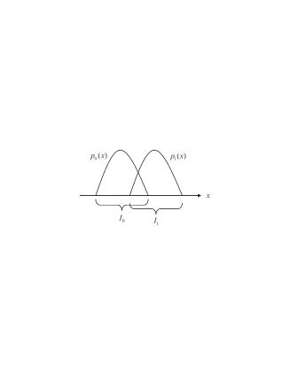
Figure 4: A pair of non-orthogonal classical probability distributions.

By the lights of this analogy, the task of state estimation has a natural classical analogue. Specifically, the task of correctly identifying which of a non-orthogonal pair of quantum states describes a system is analogous to the task of correctly identifying which of a non-disjoint pair of probability distributions describes a classical system, that is, of identifying whether the system was prepared by drawing its physical state at random from one or another of a pair of non-disjoint probability distributions. Just as the quantum discrimination task cannot be accomplished with certainty, neither can this classical discrimination task. The reason is that the physical state of the system has some probability of lying in the overlap of the two probability distributions (the region $I_{0}\cap I_{1}$ in Fig. 4), and this is consistent with both preparations. Thus, even a measurement that completely determined the physical state of the system could not reveal which preparation was implemented. Nonetheless, just as in quantum mechanics, there is a probability greater than 1/2 of a correct estimation, and a non-zero probability of error-free discrimination. Specifically, if one measures the physical state of the system, and finds it in the region outside the overlap of the distributions (outside of $I_{0}\cap I_{1}$), then one knows with certainty which distribution describes the system.

Similarly, there is a classical analogue for the task of state targeting. The target quantum state is replaced by a target probability distribution. Alice submits a system to Bob, then learns the identity of the target distribution, announces a distribution to Bob, and Bob tests the submitted system for being described by the announced distribution. The simplest way for Bob to test for a distribution is to test the system for being in the support of the distribution, that is, for being in the subset of the physical state space that is assigned non-zero probability by the distribution. For instance, one tests for $p_{b}(x)$ by verifying whether $x$ lies in region $I_{b}$, depicted in Fig. 4. It is now clear that Alice can achieve some non-trivial control. For instance, if she initially submits a system prepared according to $p_{0}(x)$, but the target distribution is $p_{1}(x)$, then she still has some probability of passing a test for $p_{1}(x)$. Specifically, her probability is the integral of $p_{0}(x)$ in the region $I_{0}\cap I_{1}$.

For both state estimation and state targeting, there are differences between what can be achieved in the quantum and the classical contexts.

In the case of estimation of classical probability distributions, one does not necessarily alter the probability distribution by acquiring information about it, and thus one does not alter the probability of passing subsequent tests. For instance, if the distribution is $p_{b}(x)$, then the fact that someone measures whether $x$ is in the interval $I_{0}$ or not does not change the fact that the system will be found in the interval $I_{b}$ when tested. On the other hand, gaining information about which of a pair of non-orthogonal states describes a quantum system does influence the probability that this system will subsequently pass a test for the state in which it was initially prepared.

In the case of classical distribution targeting, there is a strategy that allows one to pass the test for the target state with certainty. For instance, if the target distribution is one of $p_{0}(x)$ or $p_{1}(x)$, then Alice can simply prepare the system in a physical state $x\in I_{0}\cap I_{1}$ and be certain to pass both the test for $p_{0}(x)$ (being in the interval $I_{0}$) and the test for $p_{1}(x)$ (being in the interval $I_{1}$). One can say that Alice achieves complete control in this case. On the other hand, in the quantum case, such complete control is not possible because no quantum state can pass the test for each of two non-orthogonal pure states with certainty.

Thus, if one takes the view that quantum states are states of knowledge, what is surprising about quantum state estimation is not that one cannot achieve an error-free discrimination of non-orthogonal states with certainty but rather that one cannot gain information without incurring a disturbance. Similarly, what is surprising about quantum state targeting is not the possibility of achieving a non-trivial control, but rather the impossibility of achieving complete control, that is, the impossibility of achieving successful state targeting with probability 1, since this is what one would expect from examining the analogous classical task.

Recognizing this difference between the classical and quantum tasks is likely to be useful in devising quantum information processing protocols that are provably superior to their classical counterparts.

Appendix A Derivation of Eqs. (9) and (10)

If the states $\rho,$ $\left|\psi_{0}\right\rangle$ and $\left|\psi_{1}\right\rangle$ are represented by Bloch vectors $\vec{r},$ $\hat{a}_{0},$ and $\hat{a}_{1}$ respectively, then $1/\left\langle\psi_{b}\right|\rho^{-1}\left|\psi_{b}\right\rangle$ $=(1-\left|\vec{r}\right|^{2})/2(1-\vec{r}\cdot\hat{a}_{b}),$ and Eq. (8) becomes

$$C_{\mathrm{df}}=\frac{1}{4}(1-\left|\vec{r}\right|^{2})\left(\frac{1}{1-\vec{r}\cdot\hat{a}_{0}}+\frac{1}{1-\vec{r}\cdot\hat{a}_{1}}\right).$$ (31)

Extremizing $C_{\mathrm{df}}$ with respect to variations in $\vec{r},$ we obtain

$$(1-\vec{r}\cdot\hat{a}_{0})^{2}\left((1-\vec{r}\cdot\hat{a}_{0})2\vec{r}+(1-\left|\vec{r}\right|^{2}\hat{a}_{0}\right)$$

$$+(1-\vec{r}\cdot\hat{a}_{1})^{2}\left((1-\vec{r}\cdot\hat{a}_{1})2\vec{r}+(1-\left|\vec{r}\right|^{2}\hat{a}_{1}\right)$$

$$= 0$$

One can then easily verify that the solution, $\vec{r}^{\text{opt}},$ lies on the bisector of $\hat{a}_{0}$ and $\hat{a}_{1},$ that is, $\vec{r}^{\text{opt}}\cdot(\hat{a}_{0}\times\hat{a}_{1})=0$ and $\vec{r}^{\text{opt}}\cdot\hat{a}_{0}=\vec{r}^{\text{opt}}\cdot\hat{a}_{1},$ or equivalently,

$$\vec{r}^{\text{opt}}=\left|\vec{r}^{\text{opt}}\right|\frac{\hat{a}_{0}+\hat{a}_{1}}{\left|\hat{a}_{0}+\hat{a}_{1}\right|}$$ (32)

and has length

$$\left|\vec{r}^{\text{opt}}\right|=\sqrt{\frac{2}{1+\hat{a}_{0}\cdot\hat{a}_{1}}}\left(1-\sqrt{\frac{1-\hat{a}_{0}\cdot\hat{a}_{1}}{2}}\right).$$ (33)

Translating these expressions from the Bloch sphere representation to the Hilbert space representation yields Eq. (10). Finally, plugging $\vec{r}^{\text{opt}}$ into Eq. (31) we obtain Eq. (9).

Appendix B Comparison between convex decomposition tests and purification tests

The purification test for the mixed state $\sigma_{b}$ is a PVM measurement $\{E_{b},I-E_{b}\}$ where

$$E_{b}=\left|\psi_{b}\right\rangle\left\langle\psi_{b}\right|$$ (34)

with $\left|\psi_{b}\right\rangle$ a purification of $\sigma_{b}$. Alice’s maximum control in state targeting for two mixed states, $\sigma_{0}$ and $\sigma_{1},$ assuming purification tests is

$$C_{\text{pur}} = \max_{\left|\psi\right\rangle,U_{0},U_{1}}\sum_{b=0}^{1}\tfrac{1}{2}\mathrm{Tr}\left(E_{b}(I\otimes U_{b})\left|\psi\right\rangle\left\langle\psi\right|(I\otimes U_{b}^{{\dagger}})\right)$$

$$= \max_{\left|\psi\right\rangle,U_{0},U_{1}}\sum_{b=0}^{1}\tfrac{1}{2}\left|\langle\psi_{b}\right|(I\otimes U_{b})\left|\psi\rangle\right|^{2}$$

$$= \max_{\rho}\left(\frac{1}{2}F(\sigma_{0},\rho)^{2}+\frac{1}{2}F(\sigma_{1},\rho)^{2}\right).$$

where we have used Uhlmann’s theorem, Eq. (18). Note that the choice of purifications is unimportant since the probability of passing the test does not depend on this choice; the optimization yields an expression depending only on the reduced density operators.

Suppose $\sigma_{b}$ has a convex decomposition $\{(p_{b,k},\left|\phi_{b,k}\right\rangle)\}$. Typically, in a convex decomposition test Alice sends Bob a classical message containing $b$ and $k,$ and then Bob measures the projector onto $\left|\phi_{b,k}\right\rangle.$ However, one can think of Alice’s classical message as being conveyed by an orthogonal set of states $\{|b,k\rangle\}$ of a quantum “message” system, and the measurement on the system may be made conditional upon the state of this message system. Thus, one can understand the convex decomposition test for $\sigma_{b}$ as a PVM mesurement $\{G_{b},I-G_{b}\}$ where

$$G_{b}=\sum_{k}\left|b,k\right\rangle\left\langle b,k\right|\otimes\left|\phi_{b,k}\right\rangle\left\langle\phi_{b,k}\right|.$$ (35)

Alice’s maximum control for such a test is

$$C_{\text{con}}=\max_{\left|\psi\right\rangle,U_{0},U_{1}}\sum_{b=0}^{1}\tfrac{1}{2}\mathrm{Tr}\left(G_{b}(I\otimes U_{b})\left|\psi\right\rangle\left\langle\psi\right|(I\otimes U_{b}^{{\dagger}})\right)$$ (36)

Now, note that the state

$$\left|\chi_{b}\right\rangle=\sum_{k}\sqrt{p_{b,k}}\left|b,k\right\rangle\left|\phi_{b,k}\right\rangle,$$ (37)

which is a purification of $\sigma_{b},$ is an eigenstate of $G_{b}$. Thus,

$$G_{b}=\left|\chi_{b}\right\rangle\left\langle\chi_{b}\right|+\Gamma,$$ (38)

for some positive operator $\Gamma.$

It follows that for positive $A,$ Tr$(G_{b}A)\geq\mathrm{Tr}(\left|\chi_{b}\right\rangle\left\langle\chi_{b}\right|A).$ Using this, we obtain

$$C_{\text{con}}\geq\max_{\left|\psi\right\rangle,U_{0},U_{1}}\sum_{b=0}^{1}\tfrac{1}{2}\left\langle\chi_{b}\right|(I\otimes U_{b})\left|\psi\right\rangle$$ (39)

But because the probability of passing a purification test is independent of the choice of purifications, the right hand side is simply $C_{\text{pur}},$ and we have

$$C_{\text{con}}\geq C_{\text{pur}}.$$ (40)

Thus, state targeting with convex decomposition tests is always as easy, or easier, than state targeting with purification tests.

Appendix C Derivation of Eqs. (20) and (21)

We begin by deriving Eq. (20), i.e. that the fidelity satisfies

$$\max_{\rho}\left(F^{2}\left(\rho,\sigma\right)+F^{2}\left(\rho,\omega\right)\right)=1+F\left(\sigma,\omega\right).$$ (41)

By Uhlmann’s theorem we can re-express the left-hand side of Eq. (41) in terms of arbitrary purifications $\left|\psi\right\rangle,\left|\chi\right\rangle$ and $\left|\phi\right\rangle$ of $\rho,$ $\sigma$ and $\omega,$

$$\text{LHS}=\max_{\left|\psi\right\rangle}\left(\max_{U}\left|\left\langle\chi\right|U\otimes I\left|\psi\right\rangle\right|^{2}+\max_{V}\left|\left\langle\phi\right|V\otimes I\left|\psi\right\rangle\right|^{2}\right).$$ (42)

We now invert the order of the maximizations to obtain

$$\text{LHS}=\max_{U,V}\max_{\left|\psi\right\rangle}\left(\left|\left\langle\chi^{\prime}|\psi\right\rangle\right|^{2}+\left|\left\langle\phi^{\prime}|\psi\right\rangle\right|^{2}\right),$$ (43)

where

$$\left|\chi^{\prime}\right\rangle = U^{{\dagger}}\otimes I\left|\chi\right\rangle$$

$$\left|\phi^{\prime}\right\rangle = V^{{\dagger}}\otimes I\left|\phi\right\rangle.$$

This becomes

LHS $$= \max_{U,V}\max_{\left|\psi\right\rangle}\left|\left\langle\psi|\left(\left|\chi^{\prime}\right\rangle\left\langle\chi^{\prime}\right|+\left|\phi^{\prime}\right\rangle\left\langle\phi^{\prime}\right|\right)|\psi\right\rangle\right|$$

$$= \max_{U,V}\lambda^{\max}(\left|\chi^{\prime}\right\rangle\left\langle\chi^{\prime}\right|+\left|\phi^{\prime}\right\rangle\left\langle\phi^{\prime}\right|).$$

where $\lambda^{\max}(A)$ is the maximum eigenvalue of $A.$ Since

$$\lambda^{\max}\left(\left|\chi^{\prime}\right\rangle\left\langle\chi^{\prime}\right|+\left|\phi^{\prime}\right\rangle\left\langle\phi^{\prime}\right|\right)=1+\left|\left\langle\chi^{\prime}|\phi^{\prime}\right\rangle\right|.$$ (45)

we have

LHS $$= 1+\max_{U,V}\left|\left\langle\chi\right|UV^{{\dagger}}\otimes I\left|\phi\right\rangle\right|$$

$$= 1+F(\omega,\sigma),$$

where in the last step we have applied Uhlmann’s theorem, Eq. (18).  $\blacksquare$

Next, we prove Eq. (21), i.e. that the density operator $\rho$ that achieves the maximum in Eq. (41), is

$$\rho^{\text{opt}}=\frac{\omega+\sigma+\sqrt{\sigma}U\sqrt{\omega}+\sqrt{\omega}U^{{\dagger}}\sqrt{\sigma}}{2\left(1+F\left(\sigma,\omega\right)\right)},\\$$ (47)

where

$$U=\left|\sqrt{\omega}\sqrt{\sigma}\right|^{-1}\sqrt{\sigma}\sqrt{\omega}.$$ (48)

We shall require the following lemma.

Lemma

Consider two density operators, $\sigma$ and $\omega$ defined on a $d$ dimensional Hilbert space $\mathcal{H}$. Let $\mathcal{H}^{\prime}$ also be a $d$ dimensional Hilbert space. The state $\left|\phi\right\rangle\in\mathcal{H}^{\prime}\otimes\mathcal{H}$ defined by

$$\left|\phi\right\rangle=(I\otimes\sqrt{\omega})\sum_{k=1}^{d}\left|e_{k}\right\rangle\left|f_{k}\right\rangle,$$ (49)

where $\left\{\left|e_{k}\right\rangle\right\}_{k=1}^{d}$ is an orthonormal basis for $\mathcal{H}^{\prime}$ and $\left\{\left|f_{k}\right\rangle\right\}_{k=1}^{d}$ is an orthonormal basis for $\mathcal{H}^{\prime},$ is a purification of $\omega.$ Furthermore, any state of the form

$$\left|\chi\right\rangle=\left(I\otimes\sqrt{\sigma}V\right)\sum_{k=1}^{d}\left|e_{k}\right\rangle\left|f_{k}\right\rangle,$$ (50)

where $V$ is the unitary operator

$$V=\left|\sqrt{\omega}\sqrt{\sigma}\right|^{-1}\sqrt{\sigma}\sqrt{\omega}+V_{\text{null}\left(\sqrt{\omega}\sqrt{\sigma}\right)},$$ (51)

is a purification of $\sigma$ that is maximally parallel to $\left|\phi\right\rangle.$ Note that $\left|A\right|=\sqrt{A^{{\dagger}}A}$, $B^{-1}$ is the inverse of $B$ on its support, and $V_{\text{null}\left(A\right)}$ is any unitary transformation on the null space of $A.$ Note also that an arbitrary phase factor could be incorporated into $\left|\chi\right\rangle.$

Proof. It is easy to verify that $\left|\phi\right\rangle$ and $\left|\chi\right\rangle$ are indeed purifications of $\omega$ and $\sigma,$ since

$$Tr_{\mathcal{H}}\left|\phi\right\rangle\left\langle\phi\right| = \sum_{k=1}^{d}\sqrt{\omega}\left|f_{k}\right\rangle\left\langle f_{k}\right|\sqrt{\omega}$$

$$= \omega,$$

and

$$Tr_{\mathcal{H}}\left|\chi\right\rangle\left\langle\chi\right| = \sum_{k=1}^{d}\sqrt{\sigma}V\left|f_{k}\right\rangle\left\langle f_{k}\right|V^{{\dagger}}\sqrt{\sigma}$$

$$= \sqrt{\sigma}VV^{{\dagger}}\sqrt{\sigma}$$

$$= \sigma,$$

where we have used the completeness of the $\{\left|f_{k}\right\rangle\}$ and the unitarity of $V.$ Second, $\left|\phi\right\rangle$ and $\left|\chi\right\rangle$ are maximally parallel since

$$\left|\left\langle\phi|\chi\right\rangle\right|$$

$$= \left|\sum_{k}\left\langle f_{k}\right|\sqrt{\omega}\sqrt{\sigma}V\left|f_{k}\right\rangle\right|$$

$$= \left|Tr_{\mathcal{H}}\left(\sqrt{\sigma}V\sqrt{\omega}\right)\right|$$

$$= \left|Tr_{\mathcal{H}}\left(\sqrt{\sigma}\left[\left|\sqrt{\omega}\sqrt{\sigma}\right|^{-1}\sqrt{\sigma}\sqrt{\omega}+V_{\text{null}\left(\sqrt{\omega}\sqrt{\sigma}\right)}\right]\sqrt{\omega}\right)\right|$$

$$= Tr_{\mathcal{H}}\left|\sqrt{\omega}\sqrt{\sigma}\right|$$

$$= F\left(\omega,\sigma\right).$$

 $\blacksquare$

We are now in a position to prove Eq. (47). To begin, note that the $\left|\psi\right\rangle$ that achieves the maximum in Eq. (C) is simply the eigenvector of $\left|\chi^{\prime}\right\rangle\left\langle\chi^{\prime}\right|+\left|\phi^{\prime}\right\rangle\left\langle\phi^{\prime}\right|$ associated with the maximum eigenvalue,

$$\left|\psi^{\text{opt}}\right\rangle=\frac{\left|\chi^{\prime}\right\rangle+\left|\phi^{\prime}\right\rangle}{\sqrt{2}\sqrt{1+\left|\left\langle\chi^{\prime}|\phi^{\prime}\right\rangle\right|}},$$ (52)

where we have chosen phases such that $\left\langle\chi^{\prime}|\phi^{\prime}\right\rangle$ is real.

The $U$ and $V$ that achieve the maximum in Eq. (C) are any pair $U^{\text{opt}},V^{\text{opt }}$such that

$$\left|\left\langle\chi\right|U^{\text{opt}}V^{\text{opt}{\dagger}}\otimes I\left|\phi\right\rangle\right|=F(\omega,\sigma).$$ (53)

which implies that the states $\left|\chi^{\prime}\right\rangle$ and $\left|\phi^{\prime}\right\rangle$ that are defined in terms of a particular $U^{\text{opt}}$ and $V^{\text{opt }}$are maximally parallel. A particular pair of purifications of $\sigma$ and $\omega$ that are maximally parallel is provided by lemma 2. Taking Eqs. (49) and (50) to define $\left|\phi^{\prime}\right\rangle$ and $\left|\chi^{\prime}\right\rangle,$ we obtain

$$\left|\psi^{\text{opt}}\right\rangle=\frac{(I\otimes(\sqrt{\omega}+\sqrt{\sigma}V))\sum_{k=1}^{d}\left|e_{k}\right\rangle\left|f_{k}\right\rangle}{\sqrt{2}\sqrt{1+\left|\left\langle\chi^{\prime}|\phi^{\prime}\right\rangle\right|}},$$ (54)

This state allows one to achieve the maximum control. Its reduced density operator on $\mathcal{H}$ is

$$\rho^{\text{opt}} = \mathrm{Tr}_{\mathcal{H}^{\prime}}\left|\psi^{\text{opt}}\right\rangle\left\langle\psi^{\text{opt}}\right|$$

$$= \frac{(\sqrt{\omega}+\sqrt{\sigma}V)(\sqrt{\omega}+V^{{\dagger}}\sqrt{\sigma})}{2\left(1+F\left(\sigma,\omega\right)\right)}$$

$$= \frac{\omega+\sigma+\sqrt{\sigma}V\sqrt{\omega}+\sqrt{\omega}V^{{\dagger}}\sqrt{\sigma}}{2\left(1+F\left(\sigma,\omega\right)\right)}.$$

Noting that $\sqrt{\sigma}V_{\text{null}\left(\sqrt{\omega}\sqrt{\sigma}\right)}\sqrt{\omega}=\sqrt{\omega}V_{\text{null}\left(\sqrt{\omega}\sqrt{\sigma}\right)}\sqrt{\sigma}=0,$ we have the desired result.

References

- (1) C. H. Bennett and G. Brassard, in Proc. IEEE International Conference on Computers, Systems, and Signal Processing, IEEE Press, Los Alamitos (1984), p. 175.
- (2) D. Mayers, Phys. Rev. Lett. 78, 3414 (1997).
- (3) H.-K. Lo and H. F. Chau, Phys. Rev. Lett. 78, 3410 (1997).
- (4) R. W. Spekkens and T. Rudolph, Phys. Rev. A65, 012310 (2001).
- (5) R. W. Spekkens and T. Rudolph, Quantum Information and Computation 2, 66 (2002).
- (6) A. Ambainis, in Proceedings of the 33rd Annual Symposium on Theory of Computing 2001 (Association for Computing Machinery, New York, 2001), p. 134.
- (7) R. W. Spekkens and T. Rudolph, Phys. Rev. Lett. 89, 227901 (2001).
- (8) D. Aharonov et. al., in Proceedings of the 32nd Annual Symposium on Theory of Computing 2000 (Association for Computing Machinery, New York, 2000), p. 705.
- (9) H.-K. Lo, Phys. Rev. A. 56, 1154 (1997).
- (10) C.W. Helstrom, Quantum Detection and Estimation Theory (Academic Press, New York, 1976).
- (11) C. A. Fuchs, Fortschritte der Physik 46, 535 (1998); C. A. Fuchs and K. Jacobs, Phys. Rev. A. 63, 062305 (2001).
- (12) A. Einstein, B. Podolsky, and N. Rosen. Phys. Rev. 47, 777–780, 1935.
- (13) E. Schrödinger. Proc. Camb. Phil. Soc., 31, 555 (1935); Proc. Camb. Phil. Soc., 32, 446 (1936).
- (14) L.P. Hughston, R. Jozsa and W. K. Wootters, Phys. Lett. A. 183, 14 (1993).
- (15) I. Ivanovic, Phys. Lett. A. 123, 257 (1987); D. Dieks, Phys. Lett. A. 126, 303 (1988); A. Peres, Phys. Lett. A. 128, 19 (1988).
- (16) A. Peres, Quantum Theory: Concepts and Methods, (Kluwer, Dordrecht, 1995).
- (17) R. Jozsa, J. Mod. Opt. 41, 2315 (1994).
- (18) M. A. Nielsen and I. L. Chuang, Quantum Computation and Quantum Information, (Cambridge University Press, Cambridge, 2000).
- (19) A. Nayak and P. Shor, Phys. Rev. A67, 012304 (2003).
- (20) T. Rudolph,R. W. Spekkens, and P. S. Turner, Phys. Rev. A68, 010301(R), (2003).
- (21) L. Hardy and A. Kent, quant-ph/9911043 (submitted to Phys. Rev. Lett.).
- (22) C. Fuchs, quant-ph/0205039.