Interfacing quantum optical and solid state qubits

Abstract

We present a generic model of coupling quantum optical and solid state qubits, and the corresponding transfer protocols. The example discussed is a trapped ion coupled to a charge qubit (e.g. Cooper pair box). To enhance the coupling, and achieve compatibility between the different experimental setups we introduce a superconducting cavity as the connecting element.

Significant progress has been made during the last few years in implementing quantum computing proposals with various physical systemsdivincenzo_exp_quant_comp_2000 . Prominent examples are quantum optical systems, in particular trapped ionscz_gate and atoms in optical latticesJaksch_rydberg , and more recently solid state systems, such as Josephson junctionscharge_qubit_schoen ; flux_qubit_mooij and quantum dotsloss_divincenzo_dots . Among the recent experimental highlights are demonstration of, or first steps towards coherent control and read out of qubits, engineering of entanglement, and simple quantum algorithmscnot_two_ions_innsbruck ; deutsch_jozsa_innsbruck_2003 ; cnot_one_ion_nist ; nakamura_two_bits ; delft_two_bit_gates . Based on this progress, the question arises to what extent hybrid systemscpb_mechanical_resonator_schwab can be developed with the goal of combining advantages of various approaches, while still being experimentally compatible. At the heart of this problem are questions of interfacing quantum-optical qubits and solid state systems: this can be either in a form where quantum-optical qubits are connected via a solid state data bus as a route to scalable quantum computing, or by reversibly transferring a quantum optical to solid state qubits and circuits.

Below we will discuss a generic physical model and corresponding protocol for interfacing a quantum-optical and solid state charge qubit. On the quantum optics side, qubits are typically represented by long lived internal (nuclear) spin states of single atoms or ionsion_trap_decoherence_review . These single atoms can be trapped and laser cooled. External fields, provide a mechanism to manipulate the qubit, as well as to entangle the qubit with the motional state of the trapped particle. In the case of trapped ions this allows one to convert spin (the qubit) to charge superpositions, either dynamically, e.g. by kicking with a laser, or quasi-statically by applying spin-dependent (optical or magnetic) potentials. This spin to charge conversion provides a natural capacitive coupling to a solid state charge qubit, represented e.g. by a Josephson junctioncharge_qubit_schoen or a charged double quantum dotdouble_dot_rmp . Instead of direct coupling of the charges, one can introduce auxiliary elements, such as cavities. This serves the purpose of allowing increased spatial separation and mutual shielding of the systems, with the goal of easing experimental requirements for coexistence of the hybrid qubits (e.g. trapping and laser manipulation of atoms or ions), while enhancing the coupling strength in comparison with free space. Features of this hybrid system are the significantly different time scales of the evolution and coupling of the two qubits, and (in comparison with quantum optical qubits) short decoherence time of the solid state systems. We exploit this by developing a protocol of a “fast swap” with kicking by short pulses on a time scale comparable to the charge - charge coupling which is much shorter than the trap period. This has the additional benefit of being a hot gate, i.e. not requiring cooling to the motional ground state, and not making a Lamb-Dicke assumption of strong confinement.

Model for coupled qubits. A Hamiltonian for our combined system has the form $H_{t}=H_{s}+H_{q}+H_{\mathrm{int}}$ with Hamiltonian for the quantum optical qubit

$$H_{s}=\left(\frac{\hat{p}_{x}^{2}}{2m}+\frac{1}{2}m\omega_{\nu}^{2}\hat{x}^{2}\right)+\frac{\delta_{0}}{2}\sigma_{z}^{s}+\left(\frac{\hbar\omega_{R}(t)}{2}\sigma_{+}^{s}e^{i\delta k_{l}\hat{x}}+\mathrm{h.c.}\right).$$ (1)

the solid state charge qubit,

$$H_{q}=\frac{E_{z}}{2}\sigma_{z}^{q}+\frac{E_{x}}{2}\sigma_{x}^{q}$$ (2)

and interaction term

$$H_{\mathrm{int}}=\hbar\kappa(t)\hat{x}\sigma_{z}^{q}.$$ (3)

The first term in $H_{s}$ describes the $1$D-motion of a charged particle (ion) in the harmonic trapping potential with $\hat{x}$ the coordinate, $\hat{p}_{x}$ the momentum and $\omega_{\nu}$ the trapping frequency. A pseudo-spin notation with Pauli operators $\sigma_{i}^{s}$ describes the atomic qubit. Physically, the qubit is represented by two atomic ground state levels which are coupled by a laser induced Raman transition with Rabi frequency $\omega_{R}(t)$ and detuning $\delta_{0}$. Transitions between the states are associated with a momentum kick $\delta k_{l}$ due to photon absorption and emission, which couples the qubit to the motion at the Rabi frequency $\omega_{R}(t)$juanjo_fast_gate .

The Hamiltonian for the solid state charge qubit has the generic form (2) with $\sigma_{i}^{q}$ the Pauli operators, and $E_{z}$ and $E_{x}$ being tunable parameters. A Hamiltonian of this form is obtained, for example, for a superconducting charge qubit, i.e. a superconducting island connecting with a low capacitance and high resistance tunnel junction (see Fig. 1(a)). With a phase $\varphi$ and its conjugate $\hat{n}$, the Hamiltonian is $H_{q}=E_{c}(\hat{n}+C_{g}V_{g}/2e)^{2}-E_{J}\cos{\varphi}$charge_qubit_schoen , where $E_{J}$ is the Josephson energy and $E_{c}$ is the capacitive energy with $E_{c}\gg E_{J}$. The gate voltage $V_{g}$ controls the qubit through the gate capacitor $C_{g}$. The qubit forms an effective two level system with charge states $|0\rangle=|n\rangle$ and $|1\rangle=|n+1\rangle$, and $E_{z}=E_{c}(C_{g}V_{g}/2e)$ and $E_{x}=E_{J}$. Adjusting $V_{g}$ or $E_{J}$ provides arbitrary single qubit gates. Typically, $E_{c}$ is about $100\,\mathrm{GHz}$ and $E_{J}$ is about $10\,\mathrm{GHz}$. Other solid-state systems such as a double quantum dot qubit can be considered within a similar framework.

Finally, the interaction (3) has the universal form of a linear coupling via the coordinate $\hat{x}$ and the charge operator $\sigma_{z}^{q}$ which characterizes the electrostatic coupling between the motional dipole and the charge. Note that this coupling is of the order of $ep_{i}/4\pi\epsilon_{0}r_{0}^{2}$ for a given distance $r_{0}$ with dipole $p_{i}$ and charge $e$, and is a factor of $er_{0}/p_{i}$ stronger than the familiar dipole-dipole couplings encountered in quantum optics. Instead of a direct coupling of the dipole to the charge, we introduce an interaction via a short superconducting cavity. This provides a mutual shielding of the qubits, e.g. from stray photon exciting quasiparticles which might impair the coherence of the charge qubit. Furthermore, this allows the interaction to be controlled by inserting a switch, e.g. a controllable Josephson junction (a SQUID).

Coupling via a superconducting cavity. The transmission line is described by a phase variable $\psi(z,t)$ transmission_line_ref , where $z$ is the longitudinal direction of the cavity. The Lagrangian is

$$\mathcal{L}=\frac{C_{r}}{2L}\int_{0}^{L}dz\dot{\psi}^{2}-\frac{L}{2L_{r}}\int_{0}^{L}dz(\frac{\partial\psi}{\partial z})^{2},$$ (4)

with $C_{r}$ the capacitance of the cavity, $L_{r}$ the inductance, and $L$ is the length. The modes for a finite length transmission line cavity are the Fourier components of $\psi(z,t)=\sqrt{2}\sum\psi_{n}(t)\cos(kz)$ with $k=(2n+1)\pi/L$ for open boundary condition and $n$ integer. When the cavity is made of two parallel cylindrical rods with a distance $d_{0}$ and the rod radii $b_{0}$, the inductance is $L_{r}=\mu_{0}\ln{(d_{0}/b_{0})}L/\pi^{3}$ and the capacitance is $C_{r}=4\pi\epsilon_{0}L/4\ln{(d_{0}/b_{0})}$. For example, for $d_{0}=20\,\mathrm{\mu m}$, $b_{0}=1\,\mathrm{\mu m}$, $L=100\,\mathrm{\mu m}$, which gives $C_{r}=1\,\mathrm{fF}$, $L_{r}=10\,\mathrm{pH}$, the frequency of the first eigenmode of the cavity $\omega_{r}/2\pi=1.5\,\mathrm{THz}$. Application of millimeter transmission lines in the microwave regime has been proposed for the interaction of charge qubits where the cavity mode is in resonance with the qubitschoelkopf_coupling .

The coupling scheme is shown in Fig. 1(a). The left end of the cavity capacitively couples with the ion as $(V_{i}-\dot{\psi}(0,t))e\hat{x}/d_{i}$, where $d_{i}$ is the distance between the ion and the cavity and $V_{i}$ is the voltage on trap electrode. The cavity couples with one of the trap electrodes by the capacitor $C_{i}$. The right end of the cavity couples with the charge qubit via a contact capacitor $C_{m}$ as $C_{m}(\dot{\psi}(L,t)-\dot{\varphi})^{2}/2$. In our scheme, the cavity length is much shorter than the wave length of a microwave field that is characteristic of the energy of the charge qubit, so that the cavity can be represented by phases $\psi_{1,2}$ at the ends of the cavity. Each node is connected with the ground by a capacitor $C_{r}/2$, and the two nodes are connected by the inductor $L_{r}$, as is shown in Fig. 1(a). The conjugates of the phases obey the charge conservation relation $p_{1}+p_{2}=0$, where the momentum operators $p_{1,2}$ are the total charge on the nodes. With the new variable $\tilde{\psi}=\psi_{1}-\psi_{2}$ and its conjugate $\tilde{p}_{\psi}=(p_{1}-p_{2})/2$, the interaction is $H_{\mathrm{int}}=H_{\mathrm{cav}}+H_{1}$ with

$$\begin{array}[c]{c}\displaystyle H_{\mathrm{cav}}=\frac{\tilde{p}_{\psi}^{2}}{2(C_{r}/4)}+\frac{\tilde{\psi}^{2}}{2L_{r}}\\[11.38109pt] \displaystyle H_{1}=\tilde{p}_{\psi}\frac{e\hat{x}/d_{i}+C_{i}V_{i}}{C_{i}+C_{r}/2}-\tilde{p}_{\psi}\frac{C_{m}}{C_{t}}\frac{p_{\varphi}+C_{g}V_{g}}{C_{m}+C_{r}/2}\end{array}$$ (5)

where $C_{t}=C_{m}+C_{J}+C_{g},$ and we have assumed $C_{r}\gg C_{i},C_{m},C_{J},C_{g}$. The equation includes the Hamiltonian of the cavity and the coupling between the cavity, the charge and the motion. The cavity mode is an oscillator with the eigenfrequency $\omega_{r}=2/\sqrt{L_{r}C_{r}}$. With a second order perturbation approach and replacing $p_{\varphi}$ with $e\sigma_{z}^{q}$, we derive the effective coupling between the charge qubit and the ion motion,

$$H_{int}^{(2)}=\frac{e^{2}}{C_{r}}\frac{C_{m}}{C_{t}}(\frac{\hat{x}}{d_{i}}+\frac{C_{i}V_{i}}{e})(\sigma_{z}^{q}+\frac{C_{g}V_{g}}{e}),$$ (6)

where the coupling includes the effect of the gate voltage $V_{g}$ on the ion which shifts the trapping potential, and the effect of the trap voltage $V_{i}$ on the charge qubit which can be avoided by designing a balance circuit (below). The cavity shortens the distance between the charge and the ion to the order of $d_{i}$ with $\hbar\kappa=e^{2}/2C_{r}d_{i}$ where $\kappa$ is increased by a factor of $4\ln(d_{0}/b_{0})r_{0}/d_{i}$ compared with the direct coupling. With $C_{g}\sim C_{J}=0.1\,\mathrm{fF}$ and $C_{i}\sim C_{m}=0.2\,\mathrm{fF}$, $\kappa/2\pi=25\,\mathrm{GHz}/d_{i}$.

A “fast swap” gate. A controlled phase gate, $|\epsilon_{1}\rangle_{s}|\epsilon_{1}\rangle_{q}\rightarrow(-1)^{\epsilon_{1}\epsilon_{2}}|\epsilon_{1}\rangle_{s}|\epsilon_{1}\rangle_{q}$ ($\epsilon_{1,2}=0,1$), together with single qubit rotations forms a universal set of operations required for entanglement and information exchange between the ion and the charge. The swap gate, which is the key step for interfacing the ion and the charge qubit, can be achieved by three controlled phase gate together with Hadamard gates on the qubitsNielsen_Chuang_book .

We construct a phase gate operating on nanoseconds, a time scale much shorter than the trap period, and not requiring the cooling of the phonon state with a eight-pulse sequence. Three evolution operators are used in this sequence. The free evolution $U_{0}(t)=\exp{(-i\omega_{\nu}t\hat{a}_{x}^{\dagger}\hat{a}_{x})}$, where $\hat{a}_{x}$ ($\hat{a}_{x}^{\dagger}$) are the creation (annihilation) operator of the motion, is achieved by turning off the interactions $\kappa=\omega_{R}=0$ and the energy $H_{q}$. Entanglement between the motion and the spin state is obtained by applying short laser pulses with $\omega_{R}\tau_{s}=\pi$ for $n_{l}$ times ($\kappa=H_{q}=0$ and $n_{l}$ even): $U_{l}(z_{l}n_{l})=\exp{(-iz_{l}\delta k_{l}n_{l}\sigma_{z}^{s}\hat{x})}$, where $z_{k}=\pm 1$ is the direction of the photon wave vector and $\delta k_{l}$ is the momentum from one kick of the laser. The duration of the kicking $\tau_{s}$ is assumed to be much shorter than other time scales. Entanglement between the motion and the charge qubit is obtained by turning on the interaction $\kappa$ for time $\tau_{q}$ ($H_{q}=\omega_{R}=0$ and $\omega_{\nu}\tau_{q}\ll 1$): $U_{2}(\tau_{q})=\exp{(-i\kappa\tau_{q}\sigma_{z}^{q}\hat{x})}$. By flipping the charge qubit with single-qubit operation, the sign of the evolution can be flipped as $U_{2}(-\tau_{q})=\sigma_{x}^{q}U_{2}(\tau_{q})\sigma_{x}^{q}$.

The gate sequence is

$$\begin{array}[c]{c}\displaystyle U(T)=U_{l}(n_{l}^{2})U_{q}(\tau_{q}^{2})U_{0}(t_{2})U_{l}(-n_{l}^{1}-n_{l}^{2})U_{q}(-\tau_{q}^{1}-\tau_{q}^{2})\\[5.69054pt] \times U_{0}(t_{1})U_{l}(n_{l}^{1})U_{q}(\tau_{q}^{1})\end{array}$$ (7)

where the parameters fulfill $n_{l}^{1}t_{1}=n_{l}^{2}t_{2}$ and $\tau_{q}^{1}t_{1}=\tau_{q}^{2}t_{2}$. For a free particle with mass $m$ where $U_{0}(t)=\exp{(-i\hat{p}^{2}t/2m\hbar)}$, the evolution is equivalent to

$$\begin{array}[c]{c}\displaystyle U(T)=e^{-i(\hat{p}+\hbar k_{\mathrm{eff}}^{2})^{2}t_{2}/2m\hbar}e^{-i(\hat{p}-\hbar k_{\mathrm{eff}}^{1})^{2}t_{1}/2m\hbar}\\[5.69054pt] \displaystyle=e^{i\phi^{\prime}}U_{0}(t_{1}+t_{2})e^{-i\alpha\sigma_{z}^{q}\sigma_{z}^{s}}\end{array}$$ (8)

where $\phi^{\prime}$ is a global phase, $k_{\mathrm{eff}}^{i}=\delta k_{l}n_{l}^{i}\sigma_{z}^{s}+\kappa\tau_{q}^{i}\sigma_{z}^{q}$ with $i=1,2$, and $\alpha=\hbar\kappa\delta k_{l}\tau_{q}^{1}n_{l}^{1}t_{1}/mt_{2}(t_{1}+t_{2})$. The motional part factors out from the evolution of the qubits. Hence, the gate does not depend on the initial state of the phonon mode. For an oscillator by making the approximation $\exp{(-i\omega_{\nu}t)}\rightarrow 1-i\omega_{\nu}t$, the same result is obtained with the motional part replaced by $U_{0}(t_{1}+t_{2})\rightarrow\exp{(-i\omega_{\nu}(t_{1}+t_{2})\hat{a}_{x}^{\dagger}\hat{a}_{x})}$. The fidelity is $1-O(\omega_{\nu}^{2}t^{2})$ (the gate is exact for free particle) and can be increased by exploiting a low trapping frequency. For the phase gate $\alpha=\pi/4$. This gives the total gate time

$$T=\frac{\pi m}{4\hbar\kappa\delta k_{l}}(\frac{1}{n_{l}^{1}t_{1}}+\frac{1}{n_{l}^{2}t_{2}})+t_{1}+t_{2}$$ (9)

which shows that the limits of the phase gate are essentially set by the available Rabi frequency of the laser and the coupling $\kappa$. We choose $t_{1}=t_{2}=5\,\mathrm{nsec}$. With $\delta k_{l}=10^{8}\,\mathrm{m}^{-1}$, $n_{l}^{1,2}=10$, for ${{}^{9}}\mathrm{Be}^{+}$, the gate time is $T=14\,\mathrm{nsec}$; and for ${}^{43}\mathrm{Ca}^{+}$, the gate time is $T=26\,\mathrm{nsec}$, much shorter than the decoherence time of the qubits.

Decoherence of the combined system. In the interacting system of the ion, the charge qubit and the cavity, decoherence of any component affects the dynamics of the others. Decoherence of the ion trap qubit, and of the spatially separated Schrödinger cat states of ion motion, as they appear as part of our gate dynamics, is well studied ion_trap_exp_review_wineland . The dominant effect is decoherence of the charge qubit due background charge fluctuations, radiation decay, quasiparticle tunneling through the junction etc. charge_qubit_schoen . Here we concentrate on decoherence introduced by the cavity, which is the new element in the scheme, in particular the effect of excitation of quasiparticles in the superconducting transmission line generated by stray laser photons.

The dissipation of the cavity is described by a resistor $R_{r}$ in series to the inductance $L_{r}$. Following the two fluid model, the complex conductance of the superconductor is given by $\sigma(\omega)=\sigma_{1}+i\sigma_{2}$ jackson_em ; tinkham_superconductivity for $\omega$ lower than the quasiparticle gap $\Delta$, with $\sigma_{1}=n_{n}e^{2}\tau_{n}/m$ proportional to the density of normal electrons $n_{n}$, and $\sigma_{2}=n_{s}e^{2}/m\omega$ proportional to the density of superconducting electrons $n_{s}$. With the penetration depth $\lambda$ (typically of the order of microns), we obtain $R_{r}=\sigma_{1}L/\lambda\sigma_{2}^{2}b_{0}$. Without radiation, the quasiparticle density $n_{n}\sim n_{0}\mathrm{exp}(-2\Delta/k_{B}T)$ gives negligible resistance, and hence negligible dissipation ($n_{0}$ is the total electron density). However, with stray photons from the ion trap, quasiparticles are excited which leads to a resistance of $R_{r}=R_{n}(n_{ex}/n_{0})$, where $n_{ex}$ denotes the number of excited quasiparticles. The normal state resistance is $R_{n}\sim 10^{4}\,\Omega$ with given parameters.

The cavity loss can be modeled as a bosonic bath that couples to the cavity which then transfers the fluctuations to the qubits. With an imaginary time path integral approachgrabert_phys_rep , we derive the noise spectral density on the charge qubit:

$$J(\omega)=(\frac{C_{m}}{2C_{t}})^{2}\omega Z_{eff}(\omega)\coth{(\frac{\hbar\omega}{2k_{B}T})}$$ (10)

where the effective impedance $Z_{eff}$ is a capacitor $(C_{r}+C_{m})/4$ in parallel to the series of the inductor $L_{r}$ and the resistor $R_{r}$. The noise spectrum for the ion can be derived similarly.

With the fluctuation-dissipation-theorem (FDT), the decoherence rate can be derived from the spectral density. With $\omega\ll 1/\sqrt{L_{r}C_{r}}$, we have $Z_{eff}\approx R_{r}$. The decoherence rates are then

$$\gamma_{r}^{q}\approx\frac{R_{r}}{R_{k}}\frac{2k_{B}T}{\hbar}(\frac{C_{m}}{2C_{t}})^{2},\quad\gamma_{r}^{x}\approx\frac{R_{r}}{R_{k}}\frac{2k_{B}T}{\hbar}(\frac{x_{r}}{4d_{i}})^{2},$$ (11)

where $R_{k}=\hbar/(2e)^{2}$ is the quantum resistance and $x_{r}$ is the spatial displacement of the dipole. Consider the laser power of mW, and assume the absorbed power to be nW for a duration of $100\,\mathrm{nsec}$. We have $R_{r}=R_{n}/10^{5}$. With the temperature $T=100\,\mathrm{mK}$, $\gamma_{r}^{q}=50\,\mathrm{msec}^{-1}$ and $\gamma_{r}^{x}=5\,\mathrm{sec}^{-1}$. This shows that the dominate decoherence is not the cavity loss compared with that of the charge qubit.

Discussion. Combining two drastically different systems naturally introduces technical questions of compatibility, such as the coexistence of an ion trap with a cavity and connected charge qubit. Ions can either be trapped with a Paul or a Penning trap, i.e. employing strong electric or magnetic fields, while a mesoscopic charge qubit can not survive a magnetic field exceeding $\sim 0.1$ Tesla and a voltage exceeding $\sim 1$ millivolt. In the case of a Paul trap typically radio frequency fields up to $250\,\mathrm{MHz}$ are applied which, according to Eq. (6), couples to the charge qubit via the capacitor $C_{i}$. For example, trapping a single ${}^{43}\mathrm{Ca}^{+}$ (${}^{9}\mathrm{Be}^{+}$) ion in a trap of the size of $\sim 20\,\mathrm{\mu m}$ ring diameter (or cap distance) requires $V_{trap}$ about $30$ - $50\,\mathrm{V}$ at $100$ - $250\,\mathrm{MHz}$ to achieve a trap depth of about $1$ - $1.5\,\mathrm{eV}$ with corresponding trap frequencies of $18$ - $20\,\mathrm{MHz}$. Thus capacitive coupling of the trap’s drive frequency to the endcaps must be carefully compensated for by using tailored eletronic filter circuits. This is only schematically indicated in Fig. 1, in all experimental setups higher order filtering is routinely used. Thus, the voltage couples to the charge qubit is now $C_{i}V_{i}+C_{ib}V_{ib}\rightarrow 0$ where only a small residue voltage due to imperfect circuitry passes to the charge qubit. With a residue of $0.1\,\mathrm{V}$ which is far off resonance, the dynamics of the qubit is not affected significantly. We note that the balance circuit requires refined electronic filtering and feedback control circuitry. In the case of a Penning trap, by using a superconducting thin film that sustains high magnetic field or by using a cavity geometry that separates the qubit from the trap, the qubit can coexist with the trap.

Coupling of two ions via a cavity. Instead of coupling an ion to a charge qubit via a cavity, we can also couple two ions, albeit at the expense of a reduced coupling strength. This provides an alternative to the standard scenarios of scalable quantum computing with trapped ions, which are based on moving ions large_scale_wineland ; cz_gate_2000 . With the geometry according to Fig. 1(a), the ions couple to the ends of the cavity. The ion-ion Hamiltonian can be derived similar to above as

$$H_{i-i}=H_{s}^{1}+H_{s}^{2}+\frac{e^{2}}{2(C_{r}+2C_{i})}\frac{\hat{x}_{1}\hat{x}_{2}}{d_{i}^{2}}$$ (12)

where $H_{s}^{1,2}$ are the Hamiltonian for the two ions defined in Eq. (1), and the trap voltage can be included by replacing $e\hat{x}_{1,2}/d_{i}\rightarrow$ $e\hat{x}_{1,2}/d_{i}+C_{i}V_{i}$. With an laser induced dipole of $ex_{r}$, the interaction magnitude is $4\ln{(d_{0}/b_{0})}e^{2}x_{r}^{2}/4\pi\epsilon_{0}d_{i}^{2}L$. Compared with the direct (free space) coupling between two dipoles with a distance $L$, the interaction is enhanced by a factor $4\ln{(d_{0}/b_{0})}(L/d_{i})^{2}$. Besides, the coupling has the advantage of being switchable: by inserting a switch, e.g. a tunable Josephson junction, in the circuit, the interaction can be turned on and off in picoseconds. The coupling is in principle scalable by fabricating multiple connected cavities.

To conclude, we have studied a generic model and protocol for coupling qubits stored in trapped ions and solid state charge qubits via a coaxial cavity. The present example illustrates prospects of combining and interfacing quantum optical and solid state systems, and may open new routes towards scalable quantum computing.

Note added: After completion of this work, we found the preprint quant-ph/0308145, by A. S. Sorensen and et al, discussing coupling Rydberg atoms resonantly to superconducting transmission line.

Acknowledgments: Work at the University of Innsbruck is supported by the Austrian Science Foundation, European Networks and the Institute for Quantum Information.

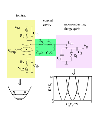
Figure 1: Schematic coupling circuit of the charge qubit and trapped ion. Top: the coupling via a cavity. The voltage at the electrode is balanced by a filtering circuit. Bottom left: coherent states of the motional mode. Bottom right: energy of charge qubit vs gate voltage.

References

- (1) D. P. DiVincenzo, in Fortsch. Phys. vol 48, special issue on Experimental Proposals for Quantum Computation (2000), also available at quant-ph/0002077.
- (2) J. I. Cirac and P. Zoller, Phys. Rev. Lett. 74, 4091 (1995).
- (3) D. Jaksch and et al, Phys. Rev. Lett. 85, 2208 (2000).
- (4) Y. Makhlin, G. Schön, and A. Shnirman, Rev. Mod. Phys. 73, 357 (2001).
- (5) J.E. Mooij and et al, Science 285, 1036 (1999).
- (6) D. Loss and D. P. DiVincenzo, Phys. Rev. A 57, 120 (1998).
- (7) F. Schmidt-Kaler and et al, Nature 422, 408 (2003).
- (8) S. Gulde and et al, Nature 421, 48 (2003).
- (9) D. Leibfried and et al, Nature 422, 412 (2003).
- (10) Yu. A. Pashkin and et al, Nature 421, 823 (2003).
- (11) I. Chiorescu and et al, Science 299, 1869 (2003).
- (12) A. D. Armour, M. P. Blencowe, and K. C. Schwab, Phys. Rev. Lett. 88, 148301 (2002).
- (13) D. Leibfried and et al, Rev. Mod. Phys. 75, 281 (2003).
- (14) W. G. van der Wiel and et al, Rev. Mod. Phys. 75, 1 (2003).
- (15) J. J. Garcia-Ripoll, P. Zoller, and J. I. Cirac, quant-ph/0306006.
- (16) A. J. Leggett, Phys. Rev. B 30, 1208 (1984); S. Chakravarty and A. Schmid, Phys. Rev. B 33, 2000 (1986).
- (17) R. J. Schoelkopf, and et al, “The prospects for Strong Cavity QED with Superconducting Circuits”, lecture notes, Les Houches summer school (2003).
- (18) M. A. Nielson and I. L. Chuang, Quantum Computation and Quantum Information, Cambridge Univ. press (2000).
- (19) H. Grabert, P. Schramm, and G.-L. Ingold, Phys. Rep. 168, 115 (1988).
- (20) J.D. Jackson, Classical Electrodynamics, 2nd ed. John Wiley & Sons, Inc (1975).
- (21) M. Tinkham, Introduction to Superconductivity, 2nd ed. (McGraw-Hill, New York, 1996).
- (22) D. J. Wineland and et al, J. Res. Natl. Inst. Stand. Technol. 103, 259 (1998).
- (23) D. Kielpinski, C. Monroe, and D. J. Wineland, Nature 417, 709 (2002).
- (24) J. I. Cirac and P. Zoller, Nature 404, 579 (2000).