Localizable Entanglement in Antiferromagnetic Spin Chains

Abstract

Anti-ferromagnetic spin chains play an important role in condensed matter and statistical mechanics. Recently XXX spin chain was discussed in relation to information theory. Here we consider localizable entanglement. It is how much entanglement can be localized on two spins by performing local measurements on other individual spins (in a system of many interacting spins). We consider a ground state of antiferromagnetic spin chain. We study localizable entanglement [represented by concurrence] between two spins. It is a function of the distance. We start with isotropic spin chain. Then we study effects of anisotropy and magnetic field. We conclude that anisotropy increases the localizable entanglement. We discovered high sensitivity to a magnetic field in cases of high symmetry. We also evaluated concurrence of these two spins before the measurement to illustrate that the measurement raises the concurrence.

Spin chains play an important role in solid state physicse1 ; e2 ; tn ; levit ; et ; st . For example, inelastic neutron scattering on $\mbox{SrCuO}_{2}$zal can be explained by spin 1/2 Heisenberg chaines . Spin chains are also important for information theory. Recently, many-body systems attract lots of attention in the field of quantum information fazio ; jk ; bose ; vpc . Special attention has been paid to the entanglement in these systems. Entanglement plays the main role as a physical resource for quantum information and quantum computation. There is a lot in common between quantum statistical mechanics and quantum information theory. The role of phase transitions for quantum information was emphasized in Ref. fazio, . Most direct relation between correlation functions and entanglement was discovered by F. Verstraete, M. Popp and J.I. Cirac [we shall use abbreviation VPC] in Ref. vpc, . They found that correlation function provides a bound for localizable entanglement (LE).

The LE of two spins is defined as the maximal amount of entanglement that can be localized on two marked spins on average by doing local measurements on the rest of the spins [assisting spins]. Here we assume that we consider a pure state $|\phi\rangle$ of all these spins. The LE has an operational meaning applicable to situations in which one would like to concentrate as much entanglement as possible between two particular particles out of multi-particle entangled state. Good examples are quantum repeater Br98 and spinotronics loss . Let us consider an example of $N$ qubits in GHZ state:

$$|GHZ>={\frac{1}{\sqrt{2}}}(|00\ldots 0\rangle+|11\ldots 1\rangle)\ .$$ (1)

We can measure assisting qubits in $|\pm\rangle$ basis. This will force two marked spins into a Bell state [maximally entangled state of two qubits].

Let us proceed to the formal definition for localizable entanglement $E_{ij}$ between two spins marked by $i$ and $j$. Consider a pure state of $N$ spins $|\phi\rangle$ [it is normalized $\langle\phi|\phi\rangle=1$]. Every measurement basis specifies an ensemble of pure states ${\mathcal{E}}=\{p_{s},|\psi_{s}\rangle\}$. The index $s$ enumerates different measurement outcomes. It runs through $2^{(N-2)}$ values. Here $|\psi_{s}\rangle$ is a two-spin state after the measurement and $p_{s}$ is its probability. The LE is defined as

$$E_{ij}=\max_{\mathcal{E}}\sum_{s}p_{s}E(|\psi_{s}\rangle)\ .$$ (2)

Here $E(|\psi_{s}\rangle)$ is the entanglement of $|\psi_{s}\rangle$, characterized by concurrence. The concurrence $C$ was suggested by W.K. Wooterswot as a measure of entanglement . By definition it is $0\leq C\leq 1$. VPC noticed that it is in particular convenient measure for LE. It is important for us that concurrence for two qubits state $|\phi\rangle=a|00\rangle+b|01\rangle+c|10\rangle+d|11\rangle$ coincides with maximum correlation $C(|\phi\rangle)=2|ad-bc|$.

It is difficult to calculate LE. Instead, VPC found bounds for LE. The upper bound comes out of considering a global [joint] measurement on all assisting spins. It can be related to the entanglement of assistance, which is the maximum entanglement over all possible states of $N$ spins consistent with the density matrix of two marked spins. It was introduced by D.P. DiVincenzo, C.A. Fuchs, H.Mabuchi, J.A.Smolin, A.Thapliyal and A.Uhlmann div . A simple formula for entanglement of assistance was found in Ref. enk, . Let us denote the density matrix of two marked spins by $\rho_{ij}$. Matrix $X$ is a square root of the density matrix: $\rho_{ij}=XX^{\dagger}$. The entanglement of assistance measured by concurrence is given by the trace norm $tr[X^{T}(\sigma_{y}\otimes\sigma_{y})X]$. Hence, the upper bound of LE is:

$$E_{ij} \leq \frac{\sqrt{s_{+}^{ij}}+\sqrt{s_{-}^{ij}}}{2}\ ,$$ (3)

where

$$s_{\pm}^{ij} = \left(1\pm\langle\phi|\sigma_{z}^{(i)}\sigma_{z}^{(j)}|\phi\rangle\right)^{2}-\left(\langle\phi|\sigma_{z}^{(i)}|\phi\rangle\pm\langle\phi|\sigma_{z}^{(j)}|\phi\rangle\right)^{2}.$$

The lower bound on LE is expressed in terms of correlation functions:

$$Q_{\alpha\beta}^{ij} = \langle\langle\phi|\sigma_{\alpha}^{(i)}\sigma_{\beta}^{(j)}|\phi\rangle\rangle$$ (4)

$$\equiv \langle\phi|\sigma_{\alpha}^{(i)}\sigma_{\beta}^{(j)}|\phi\rangle-\langle\phi|\sigma_{\alpha}^{(i)}|\phi\rangle\langle\phi|\sigma_{\beta}^{(j)}|\phi\rangle\ .$$

The lower bound on LE is based on the following observation vpc : Given a state of $N$ spins with fixed correlation functions $Q_{\alpha\beta}^{ij}$ between two spins (marked by $i$ and $j$) and directions $\alpha$ and $\beta$, there exist directions in which one can measure other spins [assisting spins], such that this correlation does not decrease. Using this observation, VPC found a lower bound for LE:

$$E_{ij}\geq\max_{\alpha}\left(|Q_{\alpha\alpha}^{ij}|\right)\ .$$ (5)

VPC explicitly evaluated these bounds for the ground state of the Ising model and showed that actual value of LE is close to the lower bound.

In this paper we consider the ground state of infinite anti-ferromagnetic $XXX$ spin chain at zero temperature. We also consider anisotropic version: $XXZ$ chain. We calculated the concurrence before the measurement [see Appendix A] and compare it to LE. Measurement raises the concurrence.

I XXX Antiferromagnetic Spin Chain

The Hamiltonian for anti-ferromagnetic $XXX$ spin chain can be written as

$$H_{XXX}^{0}=\sum_{m}\left\{\sigma_{x}^{(m)}\sigma_{x}^{(m+1)}+\sigma_{y}^{(m)}\sigma_{y}^{(m+1)}+\sigma_{z}^{(m)}\sigma_{z}^{(m+1)}\right\}$$ (6)

Here $\sigma_{x}^{(m)}$, $\sigma_{y}^{(m)}$, $\sigma_{z}^{(m)}$ are Pauli matrix, which describe spin operators on $m$-th lattice site. Summation goes through the whole infinite lattice. The density of the Hamiltonian is a linear function of the swap gate.

Hans Bethe found eigenfunctions of the Hamiltonian of the model in 1931B . The ground state $|\phi\rangle$ was found by Hulten in Ref. H, . We shall normalize it to $1$. Correlations are defined as averages with respect to the ground state. They are isotropic

$$\langle\phi|\sigma_{\alpha}^{(i)}\sigma_{\beta}^{(j)}|\phi\rangle=\delta^{\alpha\beta}\langle\phi|\sigma_{z}^{(i)}\sigma_{z}^{(j)}|\phi\rangle\ .$$ (7)

There is no magnetization $\sigma_{\alpha}$ ($\alpha=x,y$ or $z$)

$$\sigma_{\alpha}=\langle\phi|\sigma_{\alpha}^{(j)}|\phi\rangle=0\ .$$ (8)

This simplifies the lower bound (5) of LE :

$$1\geq E_{ij}\geq|\langle\phi|\sigma_{z}^{(i)}\sigma_{z}^{(j)}|\phi\rangle|\ .$$ (9)

Let us now use the explicit expression for correlations $\langle\phi|\sigma_{z}^{(i)}\sigma_{z}^{(j)}|\phi\rangle$ to calculate the lower bound:

$$\langle\phi|\sigma^{(m)}_{z}\sigma^{(m+1)}_{z}|\phi\rangle = \frac{1}{3}-\frac{4}{3}\ln 2\simeq-0.5908629072\ ,$$ (10)

$$\langle\phi|\sigma^{(m)}_{z}\sigma^{(m+2)}_{z}|\phi\rangle = \frac{1}{3}-\frac{16}{3}\ln 2+3\zeta(3)$$ (11)

$$\simeq 0.2427190798\ ,$$

$$\langle\phi|\sigma_{z}^{(m)}\sigma_{z}^{(m+3)}|\phi\rangle = \frac{1}{3}-12\ln 2+\frac{74}{3}\zeta(3)-\frac{56}{3}\zeta(3)\ln 2$$ (12)

$$-6\zeta(3)^{2}-\frac{125}{6}\zeta(5)+\frac{100}{3}\zeta(5)\ln 2$$

$$\simeq -0.2009945090\,$$

$$\langle\phi|\sigma_{z}^{(m)}\sigma_{z}^{(m+4)}|\phi\rangle = \frac{1}{12}-\frac{16}{3}\ln 2-54\ln 2\,\zeta(3)-$$ (13)

$$\frac{293}{4}\zeta^{2}(3)-\frac{875}{12}\zeta(5)+\frac{145}{6}\zeta(3)$$

$$+\frac{1450}{3}\ln 2\,\zeta(5)-\frac{275}{16}\zeta(3)\zeta(5)$$

$$-\frac{1875}{16}\zeta^{2}(5)+\frac{3185}{64}\zeta(7)-$$

$$\frac{1715}{4}\ln 2\zeta(7)+\frac{6615}{32}\zeta(3)\zeta(7)$$

$$\simeq 0.0346527769.$$

It took a long time to evaluate correlations functions. Nearest neighbor correlation can be extracted from the ground state energyH . Next to nearest neighbor correlation was calculated by M. Takahashi in 1977, see Ref. Takahashi77, . Recently it was established that all correlations can be expressed as polynomials of $\ln 2$ and the values of Riemann zeta function at odd argumentsbk1 ; bk2 ; bkns ; bks ; bks2 ; bks3 . These polynomials have only rational coefficients. Third neighbor correlation was calculated by K. Sakai, M. Shiroishi, Y. Nishiyama, M. Takahashi , see [ssnt, ]. These results give us the following bounds for localizable entanglement [LE]:

$$E_{j,j+1} \geq 0.5908629072\ ,$$ (14)

$$E_{j,j+2} \geq 0.2427190798\ ,$$ (15)

$$E_{j,j+3} \geq 0.2009945090\ .$$ (16)

$$E_{j,j+4} \geq 0.0346527769\ .$$ (17)

At large distances correlation functions exhibits critical behavior. Asymptotic was obtained in luk ; af :

$$\langle\phi|\sigma_{z}^{(i)}\sigma_{z}^{(j)}|\phi\rangle\to(-1)^{i-j}\left\{\frac{(2\ln|i-j|)^{1/2}}{(\pi)^{3/2}|i-j|}\right\}.$$ (18)

This helps us to estimate localizable entanglement asymptotically for two spins, which are far away, i.e. $|i-j|\rightarrow\infty$:

$$E_{ij}\geq\left\{\frac{(2\ln|i-j|)^{1/2}}{(\pi)^{3/2}|i-j|}\right\}\ .$$ (19)

Even better, but more complicate expression for lower bound of LE , can be extracted from the paper lt :

$$E_{ij}\geq\sqrt{\frac{2}{\pi^{3}}}\frac{1}{|i-j|\sqrt{g}}\,\bigg{\{}\,1+\Big{(}\,\frac{3}{8}-\frac{c}{2}\,\Big{)}\,g+\Big{(}\,\frac{5}{128}-\frac{c}{16}-\frac{c^{2}}{8}\,\Big{)}\,g^{2}+\Big{(}\,\frac{21}{1024}+\frac{7c}{256}-\frac{7c^{2}}{64}-\frac{c^{3}}{16}+\frac{13\,\zeta(3)}{32}\,\Big{)}\,g^{3}+O(g^{4})\,\bigg{\}}$$

$$-\frac{(-1)^{|i-j|}}{\pi^{2}\,|i-j|^{2}}\,\bigg{\{}\,1+\frac{g}{2}+\Big{(}c+\frac{3}{4}\,\Big{)}\,\frac{g^{2}}{2}+\frac{c(c+2)}{2}\,g^{3}+O(g^{4})\,\bigg{\}}+\ldots\hskip 199.16928pt$$ (20)

Here the coupling constant $g$ depends on the distance $|i-j|$. It is defined by:

$$\sqrt{g}\,e^{\frac{1}{g}}=2\sqrt{2\pi}\,e^{\gamma_{E}+c}|i-j|\ .$$ (21)

Here $\gamma_{E}=0.5772$ is the Euler’s constant and $c$ is a parameter [normalization point]. A good choice for $c$ is $c=-1$. This boundary for LE is suitable for the full range of distances. In Appendix A we calculated concurrence before the measurement. It is nonzero only for nearest neighbors, see Ref. ch, and (88). Clearly, the measurement raises the concurrence.

II Critical XXZ antiferromagnet

Let us consider effects of anisotropy of interaction of spins. The Hamiltonian of the XXZ spin chain is:

$${\bf H}_{XXZ}^{0} = -\sum_{m}\big{\{}\sigma^{(m)}_{x}\sigma^{(m+1)}_{x}+\sigma^{(m)}_{y}\sigma^{(m+1)}_{y}$$ (22)

$$\qquad+\Delta(\sigma^{(m)}_{z}\sigma^{(m+1)}_{z}-1)\big{\}}\ .$$

We shall consider critical regime ($-1\leq\Delta<1$) and we use parametrization:

$$\Delta=\cos(\pi\eta)\ ,\qquad 0<\eta<1\ .$$ (23)

Let us remind that the case $\eta=0$ corresponds to ferromagnetic XXX, which we are not considering here. Another case $\eta=1$ corresponds to anti-ferromagnetic XXX, see previous section.

The case $\eta=2/3$ corresponds to $\Delta=-1/2$. In this case the model admits much simpler solution than generic Bethe Anzats, see Ref. s, ; rs1, ; rs2, . In this case the model is super-symmetric, see Ref. fns, .

Later we shall see that all these special cases $\eta=0,2/3,1$ have high sensitivity to magnetic field interacting with spins.

For general values of $\eta$ (23) there is no magnetization:

$$\sigma_{\alpha}=\langle\phi|\sigma_{\alpha}^{(m)}|\phi\rangle=0\ .$$ (24)

LE is bounded by maximal correlation function:

$$1\geq E_{ij}\geq\max_{\alpha}|\langle\phi|\sigma_{\alpha}^{(i)}\sigma_{\alpha}^{(j)}|\phi\rangle|\ .$$ (25)

Correlation functions decays as power laws at large distances $\ln|i-j|\gg 1/(2-2\eta)$. Leading terms of correlations are:

$$\langle\phi|\sigma_{x}^{(i)}\sigma_{x}^{(j)}|\phi\rangle = \langle\phi|\sigma_{y}^{(i)}\sigma_{y}^{(j)}|\phi\rangle=F|i-j|^{-\eta}\ ,$$

$$\langle\phi|\sigma_{z}^{(i)}\sigma_{z}^{(j)}|\phi\rangle = -{1\over\pi^{2}\eta}|i-j|^{-2}+A(-1)^{i-j}|i-j|^{-{1\over\eta}}.$$

Many people worked on the subject. Important results are obtained in luk . A good collection of references can be found in the book korepin, , see pages 512, 549-553. Since $0<\eta<1$, it becomes clear that $\sigma_{x}$ correlations asymptotically dominate the lower bound:

$$|Q_{xx}^{ij}|=|Q_{yy}^{ij}|>|Q_{zz}^{ij}|\ .$$ (26)

Finally we got the following bound for LE:

$$E_{ij}\geq F|i-j|^{-\eta}$$ (27)

This shows that anisotropy raises the lower bound for LE. The coefficient $F$ was calculatedluk ; af

$$F={1\over 2(1-\eta)^{2}}\ \biggl{[}{\Gamma\big{(}{\eta\over 2-2\eta}\big{)}\over 2\sqrt{\pi}\ \Gamma\big{(}{1\over 2-2\eta}\big{)}}\biggr{]}^{\eta}\times\qquad$$

$${\rm exp}\biggl{\{}-\int_{0}^{\infty}{dt\over t}\ \Big{(}{{\rm sinh}\big{(}\eta t\big{)}\over{\rm sinh}(t){\rm cosh}\big{(}(1-\eta)t\big{)}}-\eta e^{-2t}\Big{)}\biggr{\}}.$$ (28)

The plot is shown on Fig. 1. There is singularity in function $F$ for $\eta$ near $1$:

$$F\sim(1-\eta)^{-\frac{1}{2}}\quad\textrm{when}\quad\eta\to 1-0$$ (29)

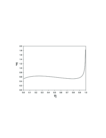
Figure 1: $F$ (Eq. 28) versus $\eta$

Special case $\eta=1$ corresponds to XXX antiferromagnet.

In Appendix A, we evaluated concurrence before the measurement. It vanishes at finite distance, see (93).

III XXX antiferromagnet in a magnetic field

Let us come back to XXX model

$$H_{XXX}^{0}=\sum_{m}\sigma_{x}^{(m)}\sigma_{x}^{(m+1)}+\sigma_{y}^{(m)}\sigma_{y}^{(m+1)}+\sigma_{z}^{(m)}\sigma_{z}^{(m+1)}\quad$$ (30)

But now let us add magnetic field

$${\bf H}_{XXX}^{h}=H_{XXX}^{0}-\sum_{m}h\sigma^{(m)}_{z}\ .$$ (31)

This introduce anisotropy in a different way. In small magnetic field $h\to 0$, small magnetization develops: $\sigma_{z}=h/\pi^{2}$. For stronger magnetic field, magnetization increases. As magnetic field approaches its critical value $h_{c}=4$, magnetization approaches $1$ [ferromagnetic state with all spins up]:

$$\sigma_{z} = 1-\frac{2}{\pi}\sqrt{h_{c}-h}\ ,\qquad h\to h_{c}-0.$$ (32)

Exact expression for magnetization $\sigma_{z}$ at arbitrary value of magnetic field is given on the pages 70-71 of the book korepin, . Averages of other spin components over ground state are zero: $\sigma_{x}=\sigma_{y}=0$.

In this section, we are considering moderate magnetic field $0\leq h\leq h_{c}$. Asymptotic of correlation functions at large distances can be described as follows:

$$\langle\langle\phi|\sigma_{z}^{(i)}\sigma_{z}^{(j)}|\phi\rangle\rangle=A_{1}\frac{1}{(i-j)^{2}}+A_{2}\frac{\cos\{\pi(1-\sigma_{z})|i-j|\}}{|i-j|^{\theta}}\quad$$ (33)

Here double bracket in the left hand side means that we subtracted $\sigma_{z}^{2}$, see (4). The coefficients $A_{1}$ and $A_{2}$ depend on magnetic field. For small magnetic field, critical index $\theta$ is close to $1$:

$$\theta = 1+[2\ln(h_{x}/h)]^{-1}\quad h\to 0;\quad h_{x}=\sqrt{\frac{8\pi^{3}}{e}}$$ (34)

and for the values of magnetic field close to critical point, $\theta$ is close to $2$:

$$\theta = 2(1-\frac{1}{\pi}\sqrt{h_{c}-h}),\quad h\to h_{c};~{}h\leq h_{c}=4.$$ (35)

In Appendix B we discuss the dependence of $\theta$ on magnetic field for intermediate fields. Fig. 4 for $\eta=1$ shows that $\theta$ is a monotonic function of the magnetic field. Asymptotic of other correlation functions are:

$$\langle\phi|\sigma^{(i)}_{x}\sigma^{(j)}_{x}|\phi\rangle=\langle\phi|\sigma^{(i)}_{y}\sigma^{(j)}_{y}|\phi\rangle=A(h)|i-j|^{-1/{\theta}}.$$ (36)

Coefficient $A(h)$ vanishes as magnetic field approaches the critical value. Exact formula for $\theta$ at any value of magnetic field can be found on the pages 73-76 of the book korepin, and in luk . It shows that $1/2\leq 1/\theta\leq 1\leq\theta\leq 2$. This means that the lower bound of LE is dominated by $\sigma_{x}$ correlations again

$$E_{ij}\geq A(h)|i-j|^{-1/{\theta}}\ .$$ (37)

Now let us discuss the upper bound (3) of LE. Because of translational invariance we have:

$$s_{+}^{ij} = \left(1+\langle\phi|\sigma_{z}^{(i)}\sigma_{z}^{(j)}|\phi\rangle\right)^{2}-4\sigma_{z}^{2}$$

$$s_{-}^{ij} = \left(1-\langle\phi|\sigma_{z}^{(i)}\sigma_{z}^{(j)}|\phi\rangle\right)^{2}\ .$$ (38)

At large space separations $|i-j|\to\infty$, correlations can be simplified $\langle\phi|\sigma_{z}^{(i)}\sigma_{z}^{(j)}|\phi\rangle\to\sigma_{z}^{2}$. This means that both $s_{\pm}^{ij}$ approach $(1-\sigma_{z}^{2})^{2}$. Finally the bounds for LE for large $|i-j|$ are

$$A(h)|i-j|^{-1/{\theta}}\leq E_{ij}<1-\sigma_{z}^{2}\ .$$ (39)

So magnetic field increases lower bound and deceases upper bound. When magnetic field are close to the critical value, the bounds become:

$$A(h)|i-j|^{-\frac{1}{2}}\leq E_{ij}<\frac{4}{\pi}\sqrt{h_{c}-h}\ .$$ (40)

In Appendix A we evaluated concurrence before the measurement. It vanishes at finite distance, see (100).

In the most general case of XXZ a magnetic field correlations can be described by the similar formulae, but parameters $h_{c}$, $\sigma_{z}$, $\theta$ are different. We shall elaborate in the next section.

IV XXZ antiferromagnet in a magnetic field

Let us add interaction with a magnetic field to XXZ spin chain:

$${\bf H}_{XXZ}^{h}=H_{XXZ}^{0}-\sum_{m}h\sigma^{(m)}_{z}\ .$$ (41)

Small magnetic field leads to a small magnetization $\sigma_{z}=\chi h$. The magnetic susceptibility $\chi$ is:

$$\chi={1-\eta\over\pi\eta\sin\pi\eta}$$ (42)

Here we used parameter $\eta$ related to anisotropy $\Delta=\cos\pi\eta$. The dependence of $\chi$ on $\eta$ is illustrated in the Fig 2.

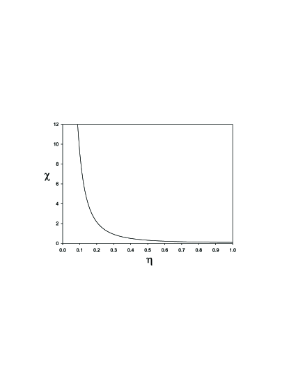
Figure 2: $\chi$ (Eq. 42) versus $\eta$ (Eq. 23)

Let us discuss the plot. The meaning of a singularity at $\eta=0$ is the following: The case $\eta=0$ corresponds to ferromagnetic XXX. At zero magnetic field it has spontaneous magnetization pointed in an arbitrary direction. Weak magnetic field will align spins to the direction of the magnetic field. This makes susceptibility infinite. As $\eta$ approaches 1, susceptibility approaches $1/\pi^{2}$ [antiferromagnetic XXX case].

For stronger magnetic field, magnetization increases. As magnetic field approaches its critical value $h_{c}=2(1-\Delta)$, magnetization approaches $1$:

$$\sigma_{z}=1-\frac{2}{\pi}\sqrt{h_{c}-h}\ ,\qquad h\to h_{c}-0.$$ (43)

Averages of other spin components over ground state are zero: $\sigma_{x}=\sigma_{y}=0$. Here we are considering moderate magnetic field $0\leq h\leq h_{c}$. Asymptotic of correlation functions at large distances can be described by the formulae similar to XXX in a magnetic field case see (33), (36), but critical index $\theta$ is different. A formula for $\theta$ depends on anisotropy $\Delta=\cos\pi\eta$. Let us first discuss small magnetic field $h\rightarrow 0$. Critical index is quadratic in magnetic field for $0\leq\eta\leq 2/3$:

$$\theta={1\over\eta}\left(1+\alpha_{1}h^{2}\right)$$ (44)

The coefficient

$$\alpha_{1}={(1-\eta)^{2}\over 4\pi\eta\tan\left({\pi\eta\over 2(1-\eta)}\right)\sin^{2}\pi\eta}$$ (45)

shows singularity at points $\eta=0$ [ferromagnetic XXX] and $\eta=2/3$ [$\Delta=-1/2$ case]:

$$\alpha_{1} \sim \frac{1}{\pi^{4}}\frac{1}{\eta^{4}}\qquad\textrm{for}\quad\eta\to 0+0$$ (46)

$$\alpha_{1} \sim \frac{1}{81\pi^{2}}\frac{1}{(\eta-2/3)}\qquad\textrm{for}\quad\eta\to\left(\frac{2}{3}\right)-0$$ (47)

The nature of dependence of the coefficient $\alpha_{1}$ is illustrated on Fig 3. In case $2/3\leq\eta\leq 1$ small $h$ behavior is more complicated:

$$\theta={1\over\eta}\left(1+\alpha_{2}h^{4(\eta^{-1}-1)}\right)$$ (48)

Notice that the power of magnetic field changes monotonically from 2 at $\eta=2/3$ to 0 at $\eta=1$. An expression for the coefficient $\alpha_{2}$ is more complicated:

$$\alpha_{2}={2\eta}e^{2\beta\over\eta}h_{0}^{4(1-\eta^{-1})}\tan\left({\pi\over\eta}\right){\Gamma^{2}\left(1+{1\over\eta}\right)\over\Gamma^{2}\left({1\over 2}+{1\over\eta}\right)}$$ (49)

Here

$$\beta=(1-\eta)\ln(1-\eta)+\eta\ln\eta$$ (50)

and

$$h_{0}={4\eta\sqrt{\pi}\sin\pi\eta\over(1-\eta)}e^{\beta\over 2(1-\eta)}{\Gamma\left({3-2\eta\over 2(1-\eta)}\right)\over\Gamma\left({2-\eta\over 2(1-\eta)}\right)}$$ (51)

$\alpha_{2}(\eta)$ shows singularity at point $\eta=2/3$

$$\alpha_{2}\sim\frac{1}{81\pi^{2}}\frac{1}{(\eta-2/3)}\qquad\textrm{for}\quad\eta\to\left(\frac{2}{3}\right)+0$$ (52)

The nature of dependence of $\alpha_{2}$ on $\eta$ is illustrated on Fig. 3.

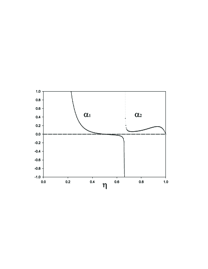
Figure 3: $\alpha_{1}$ (Eq. 45), $\alpha_{2}$ (Eq. 49) versus $\eta$ (Eq. 23)

We see that at $\eta=2/3$ critical index $\theta$ strongly depends on weak magnetic field. It also depends strongly on weak magnetic field for $\eta=1$, which is antiferromagnetic XXX case.

For magnetic field close to critical, the index $\theta$ approaches 2:

$$\theta=2+{4\sqrt{h_{c}-h}\over\pi\tan\left({\pi\eta\over 2}\right)\tan{\pi\eta}}$$ (53)

In Appendix B we discuss the dependence of $\theta$ on magnetic field for intermediate fields. Fig. 4 shows the dependence of $\theta$ on magnetic field for different values of $\eta$. Note that the dependence is monotonic.

For XXZ in a magnetic field the lower bound of localizable entanglement is also given by $\sigma_{x}$ correlations

$$E_{ij}\geq\langle\phi|\sigma^{(i)}_{x}\sigma^{(j)}_{x}|\phi\rangle$$ (54)

Asymptotic of the $\sigma_{x}$ correlations is still given by the formula (36) with $\theta$ described in this section.

V Summary

In this paper we showed that correlations in spin chains are important not only for condensed mater physics and statistical mechanics but also for quantum information. We considered boundaries for localizable entanglement in the ground state of antiferromagnetic spin chains. We showed that anisotropy raises the localizable entanglement. We also calculated concurrence before the measurement to illustrate that the measurement raises the concurrence.

There are still two open problems left: i. to prove that localizable entanglement coincide with the lower bound $E_{ij}=\max_{\alpha}\left(|Q_{\alpha\alpha}^{ij}|\right)$. ii. to calculate localizable entanglement for positive temperature.

Appendix A

In this Appendix, we calculate the concurrence between two marked spins before measurement. We show that the concurrence between $i$-th and $j$-th qubits vanishes at finite distance $|i-j|$ before the measurement. The density matrix $\rho$ of $i$-th and $j$-th spins can be represented as:

$$\rho=\frac{1}{4}\sum_{\mu_{i}}\sum_{\mu_{j}}(\sigma^{(i)}_{\mu_{i}}\otimes\sigma^{(j)}_{\mu_{j}})\langle\sigma^{(i)}_{\mu_{i}}\sigma^{(j)}_{\mu_{j}}\rangle$$ (55)

To calculate concurrence we need

$$\tilde{\rho}=(\sigma_{y}\otimes\sigma_{y})\rho^{*}(\sigma_{y}\otimes\sigma_{y}).$$ (56)

Here $\rho^{*}$ is the complex conjugate of $\rho$. Subindex $\mu$ runs though four different values $\mu=0,x,y,z$. Pauli matrix $\sigma_{\mu}$ are

$$\sigma_{0} = I=\left(\begin{array}[]{cc}1&0\\ 0&1\end{array}\right),\quad~{}\sigma_{x}=\left(\begin{array}[]{cc}0&1\\ 1&0\end{array}\right),$$ (61)

$$\sigma_{y} = \left(\begin{array}[]{cc}0&-i\\ i&0\end{array}\right),\qquad~{}~{}\sigma_{z}=\left(\begin{array}[]{cc}1&0\\ 0&-1\end{array}\right).$$ (66)

Following W.K.Wooters wot we define

$$R=\sqrt{\sqrt{\rho}\,\tilde{\rho}\,\sqrt{\rho}}$$ (67)

We shall denote the eigenvalues of $R$ by $\lambda_{k}$ in a decreasing order

$$\lambda_{1}\geq\lambda_{2}\geq\lambda_{3}\geq\lambda_{4}.$$

Then concurrence ($C$) can be expressed as

$$C=\max\{0,\lambda_{1}-\lambda_{2}-\lambda_{3}-\lambda_{4}\}.$$

Let us start with the most general case $XXZ$ in a magnetic field:

$$\langle\sigma^{(j)}_{x}\rangle=\langle\sigma^{(j)}_{y}\rangle=0;\quad\langle\sigma^{(j)}_{z}\rangle=\sigma\quad\textrm{and}\quad 0\leq\sigma<1;$$ (68)

$$\langle\sigma^{(i)}_{x}\sigma^{(j)}_{y}\rangle=0;\qquad\langle\sigma^{(i)}_{x}\sigma^{(j)}_{z}\rangle=\langle\sigma^{(i)}_{y}\sigma^{(j)}_{z}\rangle=0;$$ (69)

$$\langle\sigma^{(i)}_{x}\sigma^{(j)}_{x}\rangle=\langle\sigma^{(i)}_{y}\sigma^{(j)}_{y}\rangle=g_{x}(i-j);$$ (70)

$$\langle\sigma^{(i)}_{z}\sigma^{(j)}_{z}\rangle=G(i-j)=\sigma^{2}+g_{z}(i-j);$$ (71)

$$0<|g_{z}(i-j)|<|g_{x}(i-j)|<1\quad\mbox{for large}\quad|i-j|.$$ (72)

Hence density matrix $\rho$ for $i$-th and $j$-th qubits (spins) can be expressed as

$$\rho = \frac{1}{4}I\otimes I+\frac{g_{x}(i-j)}{4}(\sigma_{x}\otimes\sigma_{x}+\sigma_{y}\otimes\sigma_{y})$$ (73)

$$+\frac{G(i-j)}{4}\sigma_{z}\otimes\sigma_{z}+\frac{\sigma}{4}(I\otimes\sigma_{z}+\sigma_{z}\otimes I).$$

All coefficients $\sigma$, $g_{x}(i-j)$, $G(i-j)$ are real, so

$$\rho^{*} = \rho$$ (74)

$$\tilde{\rho} = (\sigma_{y}\otimes\sigma_{y})\rho(\sigma_{y}\otimes\sigma_{y})$$ (75)

First three terms in Eq. 73 commute with $\sigma_{y}\otimes\sigma_{y}$ and the last term anti-commute. Let us define

$$\rho_{0} = \frac{I\otimes I}{4}+\frac{g_{x}(i-j)}{4}(\sigma_{x}\otimes\sigma_{x}+\sigma_{y}\otimes\sigma_{y})$$ (76)

$$+\frac{G(i-j)}{4}\sigma_{z}\otimes\sigma_{z}\qquad\mbox{and}$$

$$m = \frac{\sigma}{4}(I\otimes\sigma_{z}+\sigma_{z}\otimes I).$$ (77)

Notice that $[I\otimes\sigma_{z}+\sigma_{z}\otimes I,\sigma_{x}\otimes\sigma_{x}+\sigma_{y}\otimes\sigma_{y}]=0$. So we have

$$\rho=\rho_{0}+m,\quad\tilde{\rho}=\rho_{0}-m,\quad[\rho_{0},m]=0,$$ (78)

$$~{}[\rho,m]=0,\qquad[\tilde{\rho},m]=0,\qquad[\rho,\tilde{\rho}]=0.$$ (79)

Now we can simplify the expression for the matrix $R$:

$$R=\sqrt{\sqrt{\rho}\,{\tilde{\rho}}\,\sqrt{\rho}}=\sqrt{\tilde{\rho}\,\rho}=\sqrt{\rho_{0}^{2}-m^{2}}.$$ (80)

Using this representation we can diagonalize $R$. Corresponding four eigenvalues $\{\lambda_{k}\}$ are:

$$\left\{\frac{1}{4}\sqrt{(1+G(i-j))^{2}-4\sigma^{2}},\frac{1}{4}\sqrt{(1+G(i-j))^{2}-4\sigma^{2}},\right.$$

$$\left.\frac{1-G(i-j)}{4}+\frac{g_{x}(i-j)}{2},\frac{1-G(i-j)}{4}-\frac{g_{x}(i-j)}{2}\right\}$$ (81)

Now let us consider separately special cases:

1. $XXX$ model with $h=0$.

   In this case, $\sigma=0$ and

   $$G(i-j)=g_{x}(i-j)=g_{z}(i-j)=g,$$

   The set of eigenvalues of $R$ becomes

   $$\{\lambda_{k}\}=\left\{\frac{1+g}{4},\frac{1+g}{4},\frac{1+g}{4},\frac{1-3g}{4}\right\}.$$ (82)

   To get am explicit expression for concurrence we need to consider separately two cases:

   1. $g>0$ (for $|i-j|=even$)

      $$\lambda_{1}=\lambda_{2}=\lambda_{3}=\frac{1+g}{4},\lambda_{4}=\frac{1-3g}{4}.$$ (83)

      We can calculate the concurrence $C$

      $$C=\max\{0,-\frac{1-g}{2}\}=0,$$ (84)

      since $|g|<1$.

   2. $g<0$ (for $|i-j|=odd$)

      $$\lambda_{1}=\frac{1-3g}{4},\lambda_{2}=\lambda_{3}=\lambda_{4}=\frac{1+g}{4}$$ (85)

      The concurrence

      $$C=\max\{0,\frac{-3g-1}{4}\}$$ (86)

      is non-zero only if $g<-\frac{1}{3}$. This happens only for $j=i\pm 1$ with

      $$g=\langle\sigma_{j}^{z}\sigma_{j+1}^{z}\rangle=\frac{1-4\ln 2}{3}\approx-0.591.$$ (87)

      Hence we have

      $$C_{j,j+1} = \ln 2-\frac{1}{2}\approx 0.193,$$

      $$C_{j,j+k} = 0\quad\mbox{if}\quad k>1.$$ (88)

   So, concurrence is non-zero only for nearest neighbors [for ground state of $XXX$ model without magnetic field]. It was first discovered in Ref. ch, .

2. $XXZ$ model at $h=0$.

   In this case $\sigma=0$. At $|i-j|\to\infty$

   $$g_{x}(i-j)>0,\quad g_{x}(i-j)>|g_{z}(i-j)|\quad$$

   and both $g_{x}(i-j)$ and $g_{z}(i-j)$ decay as a function of the distance $|i-j|$. Eigenvalues of $R$ become

   $$\lambda_{1}=\frac{1-g_{z}(i-j)}{4}+\frac{g_{x}(i-j)}{2};$$ (89)

   $$\lambda_{2}=\lambda_{3}=\frac{1+g_{z}(i-j)}{4};$$ (90)

   $$\lambda_{4}=\frac{1-g_{z}(i-j)}{4}-\frac{g_{x}(i-j)}{2}.$$ (91)

   Now we can calculate the concurrence:

   $$C=\max\{0,-\frac{1}{2}+g_{x}(i-j)-\frac{1}{2}g_{z}(i-j)\}$$ (92)

   It vanishes at distance larger than $|i-j|_{min}$

   $$\frac{1}{2} \simeq g_{x}(|i-j|_{min})\simeq\frac{F}{|i-j|_{min}^{\eta}};$$

   $$|i-j|_{min} \simeq (2F)^{\frac{1}{\eta}}.$$ (93)

3. $XXX$ in a magnetic field.

   $$G(i-j)=\sigma^{2}+g_{z}(i-j)$$ (94)

   For large $|i-j|$ both $g_{z}(i-j)$ and $g_{x}(i-j)$ become small. For magnetic field smaller then critical

   $$g_{z}(i-j)\frac{1+\sigma^{2}}{(1-\sigma^{2})^{2}}\ll 1$$

   $$|g_{x}(i-j)|>|g_{z}(i-j)|.$$ (95)

   Eigenvalues of $R$ in Eq. 81 become

   $$\lambda_{1}=\frac{1-\sigma^{2}}{4}-\frac{g_{z}(i-j)}{4}+|\frac{g_{x}(i-j)}{2}|;$$ (96)

   $$\lambda_{2}=\lambda_{3}=\frac{1-\sigma^{2}}{4}+\frac{g_{z}(i-j)}{4}\frac{1+\sigma^{2}}{1-\sigma^{2}};$$ (97)

   $$\lambda_{4}=\frac{1-\sigma^{2}}{4}-\frac{g_{z}(i-j)}{4}-|\frac{g_{x}(i-j)}{2}|,$$ (98)

   and concurrence becomes

   $$C=\max\{0,|g_{x}(i-j)|-\frac{1-\sigma^{2}}{2}-\frac{g_{z}(i-j)}{2}\frac{1+\sigma^{2}}{1-\sigma^{2}}\}.$$ (99)

   Hence concurrence vanishes at distance lager than $|i-j|_{min}$

   $$\frac{1-\sigma^{2}}{2} = |g_{x}(|i-j|_{min})|=|A(h)||i-j|_{min}^{-1/\theta}$$

   $$|i-j|_{min} = |\frac{2A(h)}{1-\sigma^{2}}|^{\theta}.$$ (100)

Appendix B

In this Appendix, we discuss the dependence of critical exponent $\theta$ on the magnetic field $h$. We follow the book korepin, .

1. Let us start from $XXX$ model.

   Energy of a magnon $\epsilon(\lambda)$ is defined by a set of equations:

   $$\epsilon(\lambda) - \frac{1}{2\pi}\int_{-\Lambda}^{\Lambda}K(\lambda,\mu)\epsilon(\mu)\mathrm{d}\mu=\epsilon_{0}(\lambda),$$ (101)

   $$K(\lambda,\mu) = \frac{-2}{1+(\lambda-\mu)^{2}},\quad\epsilon_{0}(\lambda)=2h-\frac{2}{\frac{1}{4}+\lambda^{2}}$$ (102)

   With extra condition $\epsilon(\pm\Lambda)=0$. This set of equation determines the dependence of $\Lambda$ on magnetic field $h$. Here $\Lambda$ is a value of a spectral parameter at the Fermi edge. An important object is the fractional charge $Z(\lambda)$:

   $$Z(\lambda)-\frac{1}{2\pi}\int_{-\Lambda}^{\Lambda}K(\lambda,\mu)Z(\mu)\mathrm{d}\mu=1.$$ (103)

   The critical exponent is equal to:

   $$\theta=2Z^{2}(\Lambda)$$ (104)

   For $XXX$ model, the critical field $h_{c}=4$. For large magnetic field ($|h|>h_{c}$) $\Lambda=0.$ If magnetic filed approaches the critical value from below, then

   $$\Lambda=\frac{1}{2}\sqrt{h_{c}-|h|}\quad\textrm{and}\quad\theta=2-\frac{4}{\pi}\Lambda\to 2.$$ (105)

   If the magnetic field is small $|h|\to 0$ then

   $$\Lambda=\frac{1}{2\pi}\ln\left(\frac{(2\pi)^{3}}{eh^{2}}\right)\to\infty\quad\textrm{and}\quad\theta=1+\frac{1}{2\pi\Lambda}\to 1$$ (106)

2. Now let us discuss $XXZ$ model.

   In this case we can use the same set of equations (101,102) with $K(\lambda,\mu)$ and $\epsilon_{0}(\lambda)$ replaced by:

   $$K(\lambda,\mu)=\frac{\sin(2\pi\eta)}{\sinh(\lambda-\mu+i\pi\eta)\sinh(\lambda-\mu-i\pi\eta)},$$

   $$\epsilon_{0}(\lambda)=2h-\frac{2\sin^{2}(\pi\eta)}{\cosh(\lambda+\frac{i\pi\eta}{2})\cosh(\lambda-\frac{i\pi\eta}{2})}.$$ (107)

   For small magnetic field

   $$\Lambda=(1-\eta)\ln\left(\frac{h_{0}}{h}\right)\to\infty\quad\textrm{when}\quad h\to 0$$ (108)

   Here $h_{0}$ is given by (51).

   But for magnetic field close to critical:

   $$\Lambda=\frac{\sqrt{h_{c}-|h|}}{2\tan(\frac{\pi\eta}{2})}\to 0\quad\textrm{when}\quad h\to\pm h_{c}.$$ (109)

   The critical value of the magnetic field is:

   $$h_{c}=2(1-\Delta)=2(1-\cos(\pi\eta))$$ (110)

   For general magnetic field $h$, we solved these equations numerically and found that both $\Lambda(h)$ and $\theta(h)$ are monotonic functions of $h$. The numerical solution for $\theta(h)$ was shown in Fig 4.

   

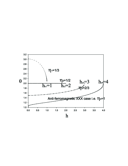
   Figure 4: Critical exponent $\theta$ (Eqs. 33 and 36) versus magnetic field $h$ for different values of anisotropy $\eta$.

References

(1) F.H.L. Essler, A. Furusaki, T. Hikihara, Dynamical Structure Factor in Cu Benzoate and other spin-1/2 antiferromagnetic
chains,
arXiv: cond-mat/0304244, Phys. Rev. B68, 064410 (2003)
(2) Y.-J. Wang, F.H.L. Essler, M. Fabrizio, A.A. Nersesyan,
Quantum criticality in a two-leg antiferromagnetic S=1/2 ladder
induced by a staggered magnetic field, arXiv: cond-mat/0112249,
Phys. Rev. B 66, 24412 (2002)
(3)A. A. Nersesyan, A. M. Tsvelik, Spinons in more than one dimension: Resonance Valence Bond state stabilized by frustration, arXiv: cond-mat/0206483
(4) L. S. Levitov, A. M. Tsvelik, Narrow gap Luttinger liquid in Carbon
nanotubes, cond-mat/0205344, Phys. Rev. Lett. 90, 016401 (2003)
(5) F.H.L. Essler (BNL), A.M. Tsvelik (BNL), Spectral function of an incommensurate Charge Density Wave State
cond-mat/0205294, Phys. Rev. Lett. 90, 126401 (2003)
(6) F. A. Smirnov, A. M. Tsvelik A Model with Propagating Spinons beyond One Dimension ,
cond-mat/0304634, Phys.Rev. B58 (1998) R8881
(8)M.A. Nielsen and I.L. Chuang, Quantum Computation And
Quantum Communication, Cambridge Univ. Press, Cambridge, 2000
(9)F. Verstraete, M. Popp and J.I. Cirac, arXiv: quant-ph/0307009, Phys. Rev. Lett. 92, 027901 (2004).
(10)B.-Q. Jin and V.E. Korepin, arXiv: quant-ph/0304108
(11)V.E. Korepin, N.M. Bogoliubov and A.G. Izergin, Quantum
inverse scattering method and correlation functions, Cambridge
Univ. Press, 1993
(12)A. Osterloh, L. Amico, G. Falci and R. Fazio
, Nature 416 608, (2002)
(13)S. Bose, arXive quant-ph/0212041, Phys. Rev. Lett. 91, 207901 (2003)
(14)H.J. Briegel et al, Phys. Rev. Lett. 81, 5932
(1998).
(15)D.D. Awschalom, D. Loss, and N. Samarth, Semiconductor Spintronics and
Quantum Computation, Springer-Verlag, Berlin, 2002.
(16) D.P. DiVincenzo, C.A. Fuchs, H.Mabuchi, J.A.Smolin, A.Thapliyal and
A.Uhlmann, arXiv: quant-ph/9803033, Proceedings of the 1st NASA International Conference on
Quantum Computing and Quantum Communication (Springer-Verlag)
(17) T. Laustsen, F. Verstraete and S. J. van Enk, arXiv: quant-ph/0206192, Quantum Information and Computation 3, 64 (2003)
(18) W.K.Wooters, Phys. Rev. Lett. 80, page 2245, 1998
(19) H. Bethe, Zeitschrift für Physik, 76, 205 (1931)
(20) L. Hulthén, Ark. Mat. Astron. Physik A26, 1
(1939)
(21) M. Takahashi,
J. Phys. C: Solid State Phys. 10 (1977) 1289
(22) H.E.Boos, V.E.Korepin, arXiv: hep-th/0104008, Journal of Physics A:
Math. Gen. V34, 5311 (2001)
(23) H.E.Boos, V.E.Korepin, hep-th/0105144, published in the book
Math.Phys Odyssey 2001 in Progress in Mathematics, dedicated to 60
birthday of Professor McCoy, Birkhauser
(24) H.E.Boos, V.E.Korepin, Y.Nishiyama and M.Shiroishi,
cond-mat/0202346, Journal of Physics A:
Math. Gen. V35, 4443 (2002)
(25) H.E.Boos, V.E.Korepin and F.A. Smirnov, Nucl.Phys.
B658, 417 (2003)
(26) H.E. Boos, V.E. Korepin, F.A. Smirnov, New formulae for solutions of quantum Knizhnik-Zamolodchikov equations on level -4 ,
J.Phys. A37 323-336 (2004), hep-th/0304077
(27) H.E. Boos, V.E. Korepin, F.A. Smirnov, New formulae for
solutions of quantum Knizhnik-Zamolodchikov equations on level -4 and
correlation functions , hep-th/0305135
(28) K. Sakai, M. Shiroishi, Y. Nishiyama, M. Takahashi, Third
Neighbor Correlators of Spin-1/2 Heisenberg Antiferromagnet,Phys.Rev. E67 (2003)
065101, cond-mat/0302564
(29) S. Lukyanov, Correlation amplitude for the XXZ spin chain
in the disordered regime, cond-mat/9809254; cond-mat/9712314, Nucl. Phys. B522 (1998), 533-549
(30) I.A. Zaliznyak, C. Broholm, M. Kibune, M.Nohara and H. Takagi,
Phys. Rev Lett. 83, 5370 (1999).
(31) M. J. Bhaseen, F. H. L. Essler, A. Grage, cond-mat/0312055
(32) I. Affleck, Exact Correlation Amplitude for the S=1/2
Heisenberg Antiferromagnetic Chain , J.Phys.A 31, 4573 (1998), cond-mat/9802045
(33) S. Lukyanov, V. Terras, Long-distance asymptotic of
spin-spin correlation functions for the XXZ spin chain , Nucl.Phys.
B654, 323-356 (2003), hep-th/0206093
(34) A. V. Razumov, Yu. G. Stroganov Spin chains and combinatorics: twisted boundary conditions, J.Phys. A34 (2001) 5335-5340 ,
cond-mat/0102247
(35) A. V. Razumov, Yu. G. Stroganov Spin chains and combinatorics, J.Phys. A34 (2001) 3185, cond-mat/0012141
(36) Yu. G. Stroganov The Importance of being Odd , J.Phys. A34 (2001) L179-L186, cond-mat/0012035
(37) P. Fendley, B. Nienhuis, K. Schoutens Lattice fermion models with super-symmetry , cond-mat/0307338, J.Phys. A36 (2003) 12399-12424
(38) S.-J. Gu, H.-Q. Li and Y.-Q. Li, Phys. Rev. A68, 042330(2003),
quant-ph/0307131.