Generation of entangled states of two atoms inside a leaky cavity

Abstract

An in-depth theoretical study is carried out to examine the quasi-deterministic entanglement of two atoms inside a leaky cavity. Two $\Lambda$-type three-level atoms, initially in their ground states, may become maximally entangled through the interaction with a single photon. By working out an exact analytic solution, we show that the probability of success depends crucially on the spectral function of the injected photon. With a cavity photon, one can generate a maximally entangled state with a certain probability that is always less than $50\%$. However, for an injected photon with a narrower spectral width, this probability can be significantly increased. In particular, we discover situations in which entanglement can be achieved in a single trial with an almost unit probability.

I Introduction

Entanglement has long been considered a fundamental property in quantum theory Schrödinger (1935); Einstein et al. (1935); Bell (1965). It has gained renewed interest due to its potential applications in quantum computations and information in recent years, and is generally considered as the corner-stone of this field (see, e.g., Refs. Bouwmeester et al. (2000); Nielsen and Chuang (2000); Raimond et al. (2001) and references therein). While entanglement can be generated by a lot of different implements such as solid-state devices Bouchiat et al. (1999); Bertoni et al. (2000); Friedman et al. (2000); van der Wal et al. (2000), nuclear magnetic resonance in liquid samples Gershenfeld and Chuang (1997); Jones et al. (1998), and ion trap Monroe et al. (1995); Turchette et al. (1998); Sackett et al. (2000), it is most conveniently realized by photons, e.g., in parametric down-conversion Yamamoto et al. (2003); Abouraddy et al. (2001). However, though being ideal carriers of quantum information, photons cannot serve as convenient storage media. The storage of information is much better implemented with atoms. In this sense, cavity quantum electrodynamics (CQED) provides a perfect stage for the interaction of information carriers and depository to take place Lange and Kimble (2000); Rauschenbeutel et al. (1999); Maître et al. (1997). With the advance in CQED technologies, some proposals have also been made to generate entangled states of atoms in optical and microwave cavities Plenio et al. (1999); Beige et al. (2000); Pachos and Walther (2002); Sørensen and Mølmer (2003); Hagley et al. (1997); Duan and Kimble (2003), many of which employ the leakage of the cavity not only as a channel for information passage, but also as the crucial element for generating entanglement Braun (2002); Plenio et al. (1999). In addition, state projection techniques using quantum measurement have also been proposed to generate entanglement in a probabilistic manner Sørensen and Mølmer (2003); Duan and Kimble (2003).

Recently, Hong and Lee have proposed a scheme to generate entangled atoms inside a leaky cavity in a “quasi-deterministic” manner Hong and Lee (2002). In their model, which is similar to that in Ref. Plenio et al. (1999), two $\Lambda$-type three-level atoms, initially prepared in their ground states, may become maximally entangled after interacting with a single cavity photon. The polarization of the output photon, serving as an indicator of the atomic state, is then measured, and generation of entangled atomic state is successful if the photon carries the right polarization. Adopting the master equation approach, they numerically showed that under the optimal condition in which the ratio of the coupling strengths of the two channels is $\sqrt{2}$, the maximum probability of success in each operation is $50\%$. They further argued that a unit probability of success can be achieved by introducing the output photon to the leaky cavity repeatedly. Through the application of this automatic feedback scheme, the two atoms in the cavity are entangled in a “quasi-deterministic” manner.

The method proposed by Hong and Lee is appealing. However, their scheme is still probabilistic for each single trial. It is therefore interesting to study whether the probability of success in each trial could be increased. The master equation approach adopted in Ref. Hong and Lee (2002) has limited further development in this direction. In addition, they obtained the optimal condition and hence the maximum probability by direct inspection on the numerical results. In the present paper, we first develop a rigorous analytic solution to their model and in turn provide a physical interpretation for the optimal condition mentioned above. We are then able to show explicitly that the upper bound $50\%$ of the probability of success is an intrinsic nature of their scheme that makes use of a cavity photon.

Furthermore, by generalizing the initial photon state to consider photons injected into the cavity with certain spectra, we find that the probability of success in each trial can be increased and larger than $50\%$. It is worthwhile to note that the master equation approach employed by Hong and Lee in Ref. Hong and Lee (2002) is not a proper description for the injected and output photons, which are usually characterized by wave packets with certain durations or, equivalently, by their respective spectral functions. The master equation approach, on the other hand, deals mainly with the “decay” of photons existing (or created) in the cavity. A photon that has already leaked out of the cavity is considered as a “decay” event and is no longer part of the system. As a consequence, their approach fails to describe the quantum states of the injected and output photons and is therefore deemed inappropriate in this situation.

In this paper, we adopt the continuous frequency mode approach that considers the cavity and its environment as a single entity to quantize the entire system Ley and Loudon (1987); Lai et al. (1988); Gea-Banacloche et al. (1990); Law et al. (2000). This enables us to study a photon with an arbitrary spectral function. We find that the probability of success in each operation depends crucially on the spectral function of the injected photon. In general, the probability can be increased to well over $50\%$. As long as spontaneous decay can be neglected, with suitably chosen spectral function of the photon, deterministic entanglement generation can be realized irrespective of the leakage rate of the cavity. Remarkably, an almost unit probability of success can be obtained for realistic CQED setups and photon packets.

The structure of our paper is as follows: In Sec. II, we introduce a proper set of spatial mode functions — the continuous frequency modes, in terms of which the electromagnetic field is quantized. The interaction Hamiltonian and the evolution of the atoms governed by it are discussed in Sec. III and IV, respectively. In Sec. V, the generation of entanglement is studied for two cases with different input states, namely, a cavity photon Lang et al. (1973); Law et al. (2000); van der Plank and Suttorp (1996) and an arbitrary injected photon. We conclude the main features of our scheme in Sec. VI.

II Continuous frequency modes

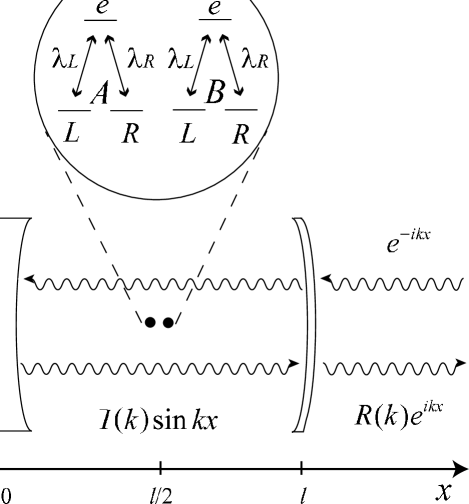
Figure 1: A sketch of the system in our model. Two $\Lambda$-type three-level atoms are trapped near the center of a one-sided leaky cavity. The continuous frequency modes shown in the figure are adopted to study the generation of atomic entangled state by a cavity mode photon or an injected photon packet.

In the following discussion we adopt the continuous frequency mode quantization scheme to analyze optical processes taking place inside a leaky optical cavity Ley and Loudon (1987); Lai et al. (1988); Gea-Banacloche et al. (1990); Law et al. (2000). Hence photons are represented by quantum states $|k_{L}\rangle$ and $|k_{R}\rangle$, which are characterized by a continuous wave number $k$, and the polarization ($L$ and $R$) of the photon. For definiteness and without loss of generality, we consider in this paper a one-sided optical cavity as shown in Fig. 1, which has length $l$ and is bounded by two mirrors. The left mirror at $x=0$ is perfectly reflecting; the right mirror at $x=l$ is partially transparent and characterized by frequency-dependent reflection and transmission coefficients $r(k)$ and $t(k)$. The spatial mode functions $U_{k}(x)$ corresponding to quantum states $|k_{L(R)}\rangle$ are given by

$$U_{k}(x)=\left\{\begin{array}[]{c}I(k)\sin{kx}\\ e^{-ikx}+R(k)e^{ikx}\end{array}\right.\begin{array}[]{ccc}{}\hfil&{}\hfil&{}\hfil\\ {}\hfil&{}\hfil&{}\hfil\end{array}\begin{array}[]{c}0<x\leq l,\\ l<x<\infty,\end{array}$$ (1)

where

$$I(k) = \frac{-2it}{1+re^{2ikl}},$$ (2)

$$R(k) = \frac{-r-t+re^{-2ikl}}{1+re^{2ikl}}.$$ (3)

Notice that $|R(k)|=1$, as required by conservation of energy. Standard Sturm-Liouville type orthogonality integral leads to the general normalization condition

$$\int_{0}^{\infty}\epsilon(x)U_{k}(x)U^{\ast}_{k^{\prime}}(x)dx=2\pi\delta(k-k^{\prime}),$$ (4)

where $\epsilon(x)$ is the position-dependent relative permittivity. For example, if an infinitely thin dielectric mirror is placed at $x=l$, then $\epsilon(x)=1+\zeta\delta(x-l)$, where $\zeta$ determines the finesse of the mirror Ley and Loudon (1987).

The quantization of the field is hence accomplished by decomposing the field operator $\hat{A}(x,t)$ into these continuous frequency modes and by introducing the usual annihilation (creation) operator $\hat{a}_{k\mu}$ ($\hat{a}^{\dagger}_{k\mu}$), with $\mu=L,R$ being the polarization index. These operators satisfy the standard commutation relation $[\hat{a}_{k\mu},\hat{a}^{\dagger}_{k^{\prime}\mu^{\prime}}]=\delta_{\mu\mu^{\prime}}\delta(k-k^{\prime})$. The result reads:

$$\hat{A}(x,t)=\sum\limits_{\mu=L,R}\int_{0}^{\infty}k^{-1/2}\left[U_{k}(x)\hat{a}_{k\mu}e^{-ikt}+U^{\ast}_{k}(x)\hat{a}^{\dagger}_{k\mu}e^{ikt}\right]dk.$$ (5)

Hereafter we adopt the cgs units and take $\hbar=c=1$.

The coefficients $I(k)$ and $R(k)$ possess poles $\tilde{k}_{n}$, which are roots of the equation $1+re^{2ikl}=0$. As long as $r(k)$ and $t(k)$ are slowly varying functions of $k$, the roots of the above equation are approximately given by: $\tilde{k}_{n}=k_{n}-i\kappa_{n}/2$, where

$$k_{n} = \frac{(2n+1)\pi-\arg\left[r(k_{n})\right]}{2l},$$ (6)

$$\kappa_{n} = -\frac{\log{|r(k_{n})|}}{l},$$ (7)

and $n=0,\pm 1,\pm 2,\ldots$ . These complex frequencies define the quasi-modes of the cavity Ley and Loudon (1987); Lai et al. (1988); Gea-Banacloche et al. (1990); Ching et al. (1998). Figure 2 shows a sketch of $|U_{k}(x_{0})|^{2}$ versus $k$ at a point $x_{0}$ inside the cavity. Each peak in the figure corresponds to a quasi-mode of the cavity. For large $n$, the separations and widths of the modes can be taken as constants given by $\pi/l$ and $\kappa$, respectively. The physical significance of these quasi-modes is that for a “good cavity”, where $|r|\simeq 1$, the mode function is negligibly small except at frequencies $k\simeq k_{n}$. In fact, it can be shown that the electrodynamics inside the cavity is completely describable in terms of these quasi-modes Ching et al. (1998). In the following, we shall make use of this formalism to discuss the interaction between the atoms and the quantized photon field.

III Atom-field interaction

We consider two identical $\Lambda$-type atoms $A$ and $B$ located near the center of a one-sided cavity as shown in Fig. 1. The separation of the atoms is assumed to be much smaller than the wavelength of the field in interest. The two ground states and the excited state are, respectively, denoted by $|L_{\alpha}\rangle$, $|R_{\alpha}\rangle$ and $|e_{\alpha}\rangle$, where $\alpha=A$, $B$ refers to atom $A$ and $B$. The excited state couples with the ground state $|L_{\alpha}\rangle$ ($|R_{\alpha}\rangle$) by emitting a $|k_{L}\rangle$ ($|k_{R}\rangle$) mode photon. In our model, we assume that the ground states are stable, and the spontaneous decay rate of the excited states into non-cavity modes is negligible compared with the cavity leakage rate $\kappa$. We shall use the notation $|\mu_{A}\mu_{B};k_{\mu}\rangle$ for states with two ground-state atoms and a single photon, where $\mu_{A}$, $\mu_{B}$, $\mu=L$, $R$ and the first and second positions are assigned to atom $A$ and $B$, respectively. States with an excited-state and a ground-state atom will similarly be denoted by $|e_{A}\mu_{B};0\rangle$ and $|\mu_{A}e_{B};0\rangle$, where $|0\rangle$ is the vacuum state of the field.

Assuming that the two ground states are degenerate and the energies of the ground and excited states are zero and $\omega_{e}$, respectively, in terms of the continuous frequency mode basis, the Hamiltonian can be written as

$$\hat{H} = \sum\limits_{\alpha=A,B}\omega_{e}|e_{\alpha}\rangle\langle e_{\alpha}|+\int_{0}^{\infty}dk\sum\limits_{\mu=L,R}\omega_{k}a_{k\mu}^{{\dagger}}a_{k\mu}$$ (8)

$$+\int_{0}^{\infty}dk\sum\limits_{\alpha=A,B\atop\mu=L,R}g_{\mu}(k)a_{k\mu}|e_{\alpha}\rangle\langle\mu_{\alpha}|+\mathrm{h}.\mathrm{c}.,$$

where the function $g(k)$ is proportional to the mode function $U_{k}(x)$ evaluated at the position of the atoms, $x_{a}\simeq l/2$.

In the present paper, the atomic frequency is assumed to be close to one of the cavity quasi-mode frequencies given by Eq. (6). Therefore, one can expand the mode functions around the resonance frequency and obtain the so-called single mode approximation result Law et al. (2000); Lang et al. (1973); van der Plank and Suttorp (1996):

$$g_{\mu}(k)=\frac{\sqrt{\kappa/2\pi}\lambda_{\mu}e^{i\theta_{\mu}}}{k-k_{c}+i\kappa/2},$$ (9)

where $k_{c}$ and $\kappa$ are, respectively, the frequency and the decay rate of the quasi-mode in resonance, and $\theta_{\mu}$ is a trivial phase angle. Besides,

$$\lambda_{\mu}^{2}=\int_{-\infty}^{\infty}|g_{\mu}(k)|^{2}dk\$$ (10)

is a measure of the coupling strength that depends on the dipole moment and the location of the atom. Also notice that within the single mode approximation, the lower limit of the frequency domain will hereafter be extended from $0$ to $-\infty$, as shown in Eq. (10).

IV Analytic solution

The system is initially prepared in the state

$$|\Psi\rangle_{\rm in}=\int_{-\infty}^{\infty}dk^{\prime}f(k^{\prime})|LL;k^{\prime}_{L}\rangle,$$ (11)

where $f(k^{\prime})$ is the spectral function of a one-photon state in the continuous frequency mode representation, satisfying the normalization condition:

$$\int_{-\infty}^{\infty}|f(k^{\prime})|^{2}dk^{\prime}=1.$$ (12)

The explicit form of the injected photon will be specified later.

We introduce an essential state basis to simplify the dynamics of the two atoms as follows. The frequency and polarization of the photon are two independent degrees of freedom of the Hilbert space. Restricted to single excitation, one of the two atoms may be excited while the other can be in $|L\rangle$ or $|R\rangle$, and thus there are four distinct states with a single excited atom. When the two atoms are in the ground states ($|L\rangle$ and $|R\rangle$ states), the polarization of the emitted photon can be either $L$ or $R$, giving rise to a total of eight distinct states for each frequency. However, if we are only interested in the evolution with the specific initial state given by Eq. (11), the dimension of the subspace involved is greatly reduced. One of the atoms in the initial state $|LL;k^{\prime}_{L}\rangle$ may absorb the photon and the state evolves into

$$|E\rangle=\frac{1}{\sqrt{2}}\left(|eL;0\rangle+|Le;0\rangle\right).$$ (13)

When the excited atom de-excites by emitting another photon of wave number $k$ ($k\neq k^{\prime}$ in general), the resulting state may be $|LL;k_{L}\rangle$ or $|\Phi;k_{R}\rangle$, where

$$|\Phi\rangle=\frac{1}{\sqrt{2}}\left(|LR\rangle+|RL\rangle\right)$$ (14)

is a Bell state of the two atoms — the goal of the current discussion. Hence, the dynamics of our system is adequately described by transitions between the excited state $|E\rangle$ and the single-photon states $|LL;k_{L}\rangle$ or $|\Phi;k_{R}\rangle$. Considering hereafter an initial state specified by Eq. (11), we obtain an effective Hamiltonian within the above-mentioned subspace:

$$\hat{H}_{\rm eff} = \omega_{e}|E\rangle\langle E|+\int_{-\infty}^{\infty}dk\,k\left(|LL;k_{L}\rangle\langle LL;k_{L}|+|\Phi;k_{R}\rangle\langle\Phi;k_{R}|\right)$$ (15)

$$+\int_{-\infty}^{\infty}dk\left(\sqrt{2}g_{L}(k)|E\rangle\langle LL;k_{L}|+g_{R}(k)|E\rangle\langle\Phi;k_{R}|\right)+\mathrm{h}.\mathrm{c}..$$

It is noteworthy that the dynamics of the current system, governed by $\hat{H}_{\rm eff}$, bears strong resemblance to that of a single $\Lambda$-type three-level system in an optical cavity, with coupling strengths of the two channels being in the ratio of $\sqrt{2}\lambda_{L}$ to $\lambda_{R}$. The factor $\sqrt{2}$ can be explained as follows. First, while both atoms in state $|LL;k_{L}\rangle$ can interact with the photon, one of the two atoms in state $|\Phi;k_{R}\rangle$ is only a spectator. Second, the collective quantum effect of the state $|\Phi\rangle$ contributes an enhancement factor $\sqrt{2}$. These two effects together give an overall $\sqrt{2}$ factor. Hence, if the coupling strengths $\lambda_{L}$ and $\lambda_{R}$ are in the ratio of $1:\sqrt{2}$, satisfying the optimal condition discovered in Ref. Hong and Lee (2002), the original two-atom model reduces to a symmetric three-level system. Interestingly enough, it is well known that a resonantly driven symmetric $\Lambda$-type atom located in an ideal cavity can exhibit perfect oscillations between its two ground states. We shall see that these analogies do shed light on our current investigation.

To simplify the calculations, we perform another basis transformation to reduce the model to a two-level system. By defining

$$|\psi_{1}(k)\rangle = \frac{1}{V(k)}\left(\sqrt{2}g_{L}^{\ast}(k)|LL;k_{L}\rangle+g_{R}^{\ast}(k)|\Phi;k_{R}\rangle\right),$$ (16)

$$|\psi_{2}(k)\rangle = \frac{1}{V(k)}\left(g_{R}(k)|LL;k_{L}\rangle-\sqrt{2}g_{L}(k)|\Phi;k_{R}\rangle\right),$$ (17)

where

$$V(k)=\sqrt{2|g_{L}(k)|^{2}+|g_{R}(k)|^{2}},$$ (18)

one of the ground states is turned into a dark state $|\psi_{2}(k)\rangle$, which does not take part in the interaction. The Hamiltonian can thus be written as

$$\hat{H}_{\rm eff}=\hat{H}_{0}+\hat{V}+\hat{H}_{\rm dark},$$ (19)

where

$$\hat{H}_{0} = \omega_{e}|E\rangle\langle E|+\int_{-\infty}^{\infty}dk\,k|\psi_{1}(k)\rangle\langle\psi_{1}(k)|,$$ (20)

$$\hat{V} = \int_{-\infty}^{\infty}dk\,V(k)|E\rangle\langle\psi_{1}(k)|+\mathrm{h}.\mathrm{c}.,$$ (21)

$$\hat{H}_{\rm dark} = \int_{-\infty}^{\infty}dk\,k|\psi_{2}(k)\rangle\langle\psi_{2}(k)|,$$ (22)

with $\hat{H}_{\rm dark}$ being the free Hamiltonian of the dark states $|\psi_{2}(k)\rangle$.

To study the output state $|\Psi\rangle_{\rm out}$ of the system subject to an arbitrary state $|\Psi\rangle_{\rm in}$ at $t=0$, we adopt the resolvent method (see, e.g Ref. Cohen-Tannoudji et al. (1992)) to deal with transitions between states with different $k$’s. Remarkably, if the trivial evolution of the dark state is discarded, the dynamics governed by the effective Hamiltonian is ostensibly analogous to that of a two-level atom interacting with a single quasi-mode. To simplify the calculation, the dark states will be ignored when solving the system using resolvent method.

The resolvent of the Hamiltonian $\hat{H}_{0}+\hat{V}$ is given by

$$\hat{G}(\omega)=\frac{1}{\omega-\hat{H}_{0}-\hat{V}},$$ (23)

with $\omega$ being a complex variable. It yields the retarded Green’s function, $\theta(t)\exp[-i(\hat{H}_{0}+\hat{V})t]$, through an integral transformation:

$$\theta(t)\exp[-i(\hat{H}_{0}+\hat{V})t]=\lim_{\epsilon\rightarrow 0^{+}}\frac{i}{2\pi}\int_{-\infty+i\epsilon}^{\infty+i\epsilon}\hat{G}(\omega)e^{-i\omega t}d\omega.$$ (24)

In the following discussion, unless otherwise stated, we assume $t>0$ and therefore identify the retarded Green’s function with the evolution operator $\hat{U}(t,0)\equiv\exp[-i(\hat{H}_{0}+\hat{V})t]$.

To evaluate the matrix elements of the resolvent, we partition the Hilbert space into two complementary parts with projection operators $\hat{P}=|E\rangle\langle E|$ and $\hat{Q}={\bf 1}-\hat{P}$. The projection of $\hat{G}(\omega)$ by $\hat{P}$ is given by Cohen-Tannoudji et al. (1992):

$$\hat{P}\hat{G}(\omega)\hat{P}=\frac{\hat{P}}{\omega-\hat{P}\hat{H}_{0}\hat{P}-\hat{P}\hat{R}(\omega)\hat{P}},$$ (25)

where $\hat{R}(\omega)$ is the level-shift operator defined as

$$\hat{R}(\omega)=\hat{V}+\hat{V}\frac{\hat{Q}}{\omega-\hat{Q}\hat{H}_{0}\hat{Q}-\hat{Q}\hat{V}\hat{Q}}\hat{V}.$$ (26)

It is then straightforward to show that

$$\langle E|\hat{R}(\omega)|E\rangle = \int_{-\infty}^{\infty}\frac{V(k)^{2}}{\omega-k}dk$$ (27)

$$= \frac{2\lambda_{L}^{2}+\lambda_{R}^{2}}{\omega-k_{c}+i\kappa/2}.$$

Hence,

$$\langle E|\hat{G}(\omega)|E\rangle = \frac{\Delta\omega+i\kappa/2}{(\Delta\omega-\delta_{e})(\Delta\omega+i\kappa/2)-2\lambda_{L}^{2}-\lambda_{R}^{2}}$$ (28)

$$= \frac{\Delta\omega+i\kappa/2}{(\Delta\omega-\omega_{+})(\Delta\omega-\omega_{-})},$$ (29)

with

$$\Delta\omega = \omega-k_{c},$$ (30)

$$\delta_{e} = \omega_{e}-k_{c},$$ (31)

and

$$\omega_{\pm}=\frac{\delta_{e}-i\kappa/2}{2}\pm\sqrt{\left(\frac{\delta_{e}+i\kappa/2}{2}\right)^{2}+2\lambda_{L}^{2}+\lambda_{R}^{2}}.$$ (32)

In our model, the atoms are in ground state at the beginning and the end. Hence the above amplitude is not of direct interest. However, this result is essential for the evaluation of the ground-state amplitudes, which is our major objective. The projection of the resolvent by $\hat{Q}$ is

$$\hat{Q}\hat{G}(\omega)\hat{Q} = \frac{\hat{Q}}{\omega-\hat{Q}\hat{H}_{0}\hat{Q}-\hat{Q}\hat{V}\hat{Q}}$$ (33)

$$+\frac{\hat{Q}}{\omega-\hat{Q}\hat{H}_{0}\hat{Q}-\hat{Q}\hat{V}\hat{Q}}\hat{V}\frac{\hat{P}}{\omega-\hat{P}\hat{H}_{0}\hat{P}-\hat{P}\hat{R}(\omega)\hat{P}}$$

$$\hat{V}\frac{\hat{Q}}{\omega-\hat{Q}\hat{H}_{0}\hat{Q}-\hat{Q}\hat{V}\hat{Q}},$$

yielding the ground-state matrix elements

$$\langle\psi_{1}(k)|\hat{G}(\omega)|\psi_{1}(k^{\prime})\rangle=\frac{\delta(k-k^{\prime})}{\omega-k}+\frac{V(k)V(k^{\prime})}{(\omega-k)(\omega-k^{\prime})}\langle E|\hat{G}(\omega)|E\rangle.$$ (34)

These expressions are generally valid Res , and can be applied to any initial photon states. In addition, when we are interested in an initial state $|\Psi\rangle_{\rm in}$ satisfying the scattering state condition:

$$\begin{array}[]{ccccc}\hat{V}e^{-i\hat{H}_{0}t}|\Psi\rangle_{\rm in}=0&&&{\rm for}&t\leq 0,\end{array}$$ (35)

then it can be shown that:

$$\langle\psi_{1}(k)|\hat{U}(t,0)|\psi_{1}(k^{\prime})\rangle = \delta(k-k^{\prime})e^{-ikt}\left[1-2\pi iV(k)^{2}\langle E|\hat{G}(k)|E\rangle\right],$$ (36)

$$= \delta(k-k^{\prime})e^{-ikt}e^{i\delta_{\rm s}(k)},$$ (37)

with $\delta_{\rm s}(k)$ being a $k$-dependent real phase shift. Equation (37) is obtained by noticing that the module of the last factor in Eq. (36) is one. While details of the proof will be given in the appendix, the physical meaning of Eq. (35) is obvious. It simply implies that the atoms do not experience the field of the injected photon as long as $t\leq 0$. Equations (36) and (37) become useful when we consider an injected photon prepared in a scattering state.

V Generation of entanglement

After interacting with the atoms, the photon leaks out of the cavity, and its polarization can be detected, e.g. by a quarter wave plate and a polarization beam splitter. The atoms inside the cavity will then be projected into either the direct product state $|LL\rangle$ or the maximally entangled state $\Phi=(|LR\rangle+|RL\rangle)/\sqrt{2}$, depending, respectively, on whether an $L$ or $R$ mode photon is detected. In the following, we consider two different cases where the photon in the initial state is (i) prepared in a cavity mode; and (ii) injected from outside with a spectral function satisfying Eq. (35).

V.1 Cavity photon

A cavity photon is identified with a quasi-mode photon as defined in Ref. van der Plank and Suttorp (1996), which is initially created inside the cavity and leaks gradually to the surroundings. In mathematical terms, a cavity photon is characterized by the spectral function:

$$f(k^{\prime})=f_{c}(k^{\prime})=\frac{1}{\lambda_{\mu}}g_{\mu}^{\ast}(k^{\prime}),$$ (38)

which corresponds to the cavity line shape. Equations (38), (16), and (17) then lead directly to

$$|\Psi\rangle_{\rm in}=\int_{-\infty}^{\infty}dk^{\prime}\frac{f_{c}(k^{\prime})}{V(k^{\prime})}\left(\sqrt{2}g_{L}(k^{\prime})|\psi_{1}(k^{\prime})\rangle+g_{R}^{\ast}(k^{\prime})|\psi_{2}(k^{\prime})\right).$$ (39)

The evolution of the dark states $|\psi_{2}(k^{\prime})\rangle$ is trivial, whereas the resolvent method gives the Fourier transform of the time evolution of the states $|\psi_{1}(k^{\prime})\rangle$. As photon detections are carried out at the end, the relevant matrix elements of the resolvent are those given by Eq. (34). Hence,

$$\langle\psi_{1}(k)|\hat{G}(\omega)|\Psi\rangle_{\rm in}=\frac{\sqrt{2}}{\omega-k}\left(\frac{g_{L}(k)f_{c}(k)}{V(k)}+\frac{\lambda_{L}\langle E|\hat{G}(\omega)|E\rangle V(k)}{\omega-k_{c}+i\kappa/2}\right),$$ (40)

and from inverse Fourier transform we obtain, as $t\rightarrow\infty$,

$$\langle\psi_{1}(k)|\hat{U}(t,0)|\Psi\rangle_{\rm in}=\sqrt{2}\left(\frac{g_{L}(k)f_{c}(k)}{V(k)}+\frac{\lambda_{L}V(k)}{(\Delta k-\omega_{+})(\Delta k-\omega_{-})}\right)e^{-ikt},$$ (41)

where all the transients have been neglected, and

$$\Delta k=k-k_{c}.$$ (42)

Notice that although we are looking at the long time behavior, Eqs. (36) and (37) do not apply to this situation because the initial state given by $f_{c}(k^{\prime})$ does not satisfy Eq. (35).

The resolvent method only solves the dynamics of the states $|\psi_{1}(k)\rangle$. The overall output state also includes the contributions of the dark states, in which a trivial phase factor $e^{-ikt}$ is multiplied. With the dark state included again, the output state in the long time limit is given by

$$|\Psi\rangle_{\rm out} = |LL\rangle\otimes\int_{-\infty}^{\infty}dk\,e^{-ikt}f_{c}(k)\frac{(\Delta k-\delta_{e})(\Delta k+i\kappa/2)-\lambda_{R}^{2}}{(\Delta k-\omega_{+})(\Delta k-\omega_{-})}|k_{L}\rangle$$ (43)

$$+|\Phi\rangle\otimes\int_{-\infty}^{\infty}dk\,e^{-ikt}f_{c}(k)\frac{\sqrt{2}\lambda_{L}\lambda_{R}e^{i\Delta_{LR}}}{(\Delta k-\omega_{+})(\Delta k-\omega_{-})}|k_{R}\rangle,$$

where

$$\Delta_{LR}=\theta_{L}-\theta_{R}.$$ (44)

If one then detects the photon in the $L$ ($R$) mode, the atomic state is projected into the non-entangled state $|LL\rangle$ (the maximally entangled state $|\Phi\rangle$), with respective probabilities $P_{L}$ and $P_{R}$ given by:

$$P_{L} = \int_{-\infty}^{\infty}\left|f_{c}(k)\frac{(\Delta k-\delta_{e})(\Delta k+i\kappa/2)-\lambda_{R}^{2}}{(\Delta k-\omega_{+})(\Delta k-\omega_{-})}\right|^{2}dk$$ (45)

$$= 1-\frac{4\lambda_{L}^{2}\lambda_{R}^{2}(2\lambda_{L}^{2}+\lambda_{R}^{2}+\kappa^{2}/2)}{(2\lambda_{L}^{2}+\lambda_{R}^{2})\left[(2\lambda_{L}^{2}+\lambda_{R}^{2}+\kappa^{2}/2)^{2}+\delta_{e}^{2}\kappa^{2}\right]},$$

$$P_{R} = 2\lambda_{L}^{2}\lambda_{R}^{2}\int_{-\infty}^{\infty}\left|\frac{f_{c}(k)}{(\Delta k-\omega_{+})(\Delta k-\omega_{-})}\right|^{2}dk$$ (46)

$$= \frac{4\lambda_{L}^{2}\lambda_{R}^{2}(2\lambda_{L}^{2}+\lambda_{R}^{2}+\kappa^{2}/2)}{(2\lambda_{L}^{2}+\lambda_{R}^{2})\left[(2\lambda_{L}^{2}+\lambda_{R}^{2}+\kappa^{2}/2)^{2}+\delta_{e}^{2}\kappa^{2}\right]}.$$

If the resonance condition is satisfied, i.e., $\delta_{e}=0$, we have

$$P_{R}=\frac{4\lambda_{L}^{2}\lambda_{R}^{2}}{(2\lambda_{L}^{2}+\lambda_{R}^{2})(2\lambda_{L}^{2}+\lambda_{R}^{2}+\kappa^{2}/2)}.$$ (47)

In strong coupling regime, where $\lambda_{L}$, $\lambda_{R}\gg\kappa$,

$$P_{R}\cong\left[\frac{2\lambda_{L}\lambda_{R}}{(2\lambda_{L}^{2}+\lambda_{R}^{2})}\right]^{2}.$$ (48)

One can easily prove that

$$P_{R}\leq\frac{1}{2}$$ (49)

and equality holds when

$$\lambda_{R}=\sqrt{2}\lambda_{L}.$$ (50)

Figure 3 shows the results of $P_{R}$ versus $\lambda_{L}/\lambda_{R}$ when $\delta_{e}=0$, and for different cavity leakage rates $\kappa/\lambda_{R}=0$, $\sqrt{2}/3$, and $7.5$. One can see that the probability depends strongly on the cavity leakage rate. For finite $\kappa$, $P_{R}$ does not attain maximum at $\lambda_{R}=\sqrt{2}\lambda_{L}$ exactly and the maximum value cannot reach $1/2$. In fact, from Eq. (47), we have,

$$P_{R}\leq\frac{2}{\left(1+\sqrt{1+(\frac{\kappa}{2\lambda_{L}})^{2}}\right)^{2}}<\frac{1}{2}$$ (51)

and equality holds when

$$\lambda_{R}=\sqrt{2}\left[1+\left(\frac{\kappa}{2\lambda_{L}}\right)^{2}\right]^{\frac{1}{4}}\lambda_{L}.$$ (52)

The above results can be better understood by studying the analog of a “three-level system” in a perfect cavity. As mentioned previously, our two-atom model reduces to a single three-level symmetric system if Eq. (50) is satisfied. It is well known that such a symmetric “three-level system”, initially in one of its ground states, oscillates between the two ground states. When $\delta_{e}=0$, the oscillations are sinusoidal and complete. When there is detuning, the evolution becomes more complicated and perfect population transfer from one ground state to the other cannot take place. However, it can be shown that when the couplings of the two channels are equal (Eq. (50) in our model), the time-averaged populations of the two ground states are equal, independent of the magnitude of detuning. Moreover, as the cavity under consideration is leaky, the probability of detecting an $L$ (or $R$) photon outside the cavity is expected to be proportional to the time the system dwelling in each of the ground states. For the case of a good cavity, the upper bound $50\%$ of the probability of success is easy to understand, as the system spends equal time on both of the ground states in this limit. Hence when the photon leaks outside the cavity, the atom has equal probability to decay into an entangled state or a direct product state.

In Ref. Hong and Lee (2002), the hyperfine levels of a cesium atom studied in Ref. Lange and Kimble (2000) were quoted as examples for realistic implementation of their scheme. Two different sets of atomic levels are studied. In both cases, $\kappa/\lambda_{R}=\sqrt{2}/3$, while $\lambda_{L}/\lambda_{R}=1$ or $\sqrt{5/6}$. The numerical results for $P_{R}$ they obtained are $0.43$ and $0.45$, respectively, which agree with our analytical solution shown by the corresponding curve in Fig. 3. In fact, from Eq. (47), our analytic results are $P_{R}=3/7$ and $9/20$, respectively.

One of the parameters in Fig. 3, $\kappa/\lambda_{R}=7.5$, is taken from a real CQED setup in Ref. Turchette et al. (1995). The parameters of the setup, when denoted by the corresponding notations in our model, are given by $(\lambda_{L(R)},\kappa,\gamma)/2\pi=(20,150,5){\rm MHz}$, where $\gamma$ is the transverse decay rate of the excited state pro . (The effect of spontaneous decay has so far been assumed negligible in our study. We shall return to discuss this point in Sec. V.2.) From Fig. 3, it is observed that in this case, the Rabi oscillation frequency is not high enough compared to the cavity leakage rate, the bias due to the initial state cannot be erased and this lowers the probability of success for poorer cavities. As can be concluded from Eq. (51), that in the weak coupling limit $\lambda_{L(R)}\ll\kappa$, $P_{R}\simeq 0$, because there is effectively no oscillation at all before the photon decays. Hence the scheme using cavity photon is implausible for weak coupling cases. However, as will be shown in Sec. V.2, the entanglement scheme still works nicely in the weak coupling regime with an injected photon.

V.2 Injected photon packet

The motivation to switch from cavity photons to injected photons is two-fold. First, it is practically more realistic to consider a photon injected into the cavity than one that already exists inside. Second, inspired by the “three-level system” analogy discussed in Sec. V.1, it is believed that an injected photon with a duration longer than the cavity leakage time may be able to “drive” the system into the entangled state with a higher efficiency. We shall see that by including general initial photon states other than cavity photon, one may also eliminate the requirement for strong coupling.

Consider an injected photon with a spectral function $f(k^{\prime})$ satisfying Eq. (35). From Eqs. (36)-(37), and following similar arguments outlined in Sec. V.1, we have

$$|\Psi\rangle_{\rm out}=|LL\rangle\otimes\int_{-\infty}^{\infty}dk\,e^{-ikt}f(k)C_{L}(k)|k_{L}\rangle-|\Phi\rangle\otimes\int_{-\infty}^{\infty}dk\,e^{-ikt}f(k)C_{R}(k)|k_{R}\rangle,$$ (53)

where

$$C_{L}(k) = \frac{(\Delta k-\delta_{e})(\Delta k^{2}+\kappa^{2}/4)-\Delta k(\lambda_{R}^{2}+2\lambda_{L}^{2})+i\kappa(\lambda_{R}^{2}-2\lambda_{L}^{2})/2}{(\Delta k-i\kappa/2)(\Delta k-\omega_{+})(\Delta k-\omega_{-})},$$ (54)

$$C_{R}(k) = \frac{\sqrt{2}ie^{i\Delta_{LR}}\kappa\lambda_{L}\lambda_{R}}{(\Delta k-i\kappa/2)(\Delta k-\omega_{+})(\Delta k-\omega_{-})}.$$ (55)

It is important to note that perfect transfer occurs at the photon frequencies

$$\Delta k=0,\,\pm\sqrt{4\lambda_{L}^{2}-\kappa^{2}/4}$$ (56)

because the corresponding amplitudes,

$$C_{L}(k) = 0,$$ (57)

$$C_{R}(k) = e^{i\Delta_{LR}},$$ (58)

as long as $\delta_{e}=0$ and Eq. (50) are satisfied. Therefore, we have an almost unit probability of generating the entangled state $|\Phi\rangle$ when $f(k)$ is strongly peaked at one of the frequencies defined in Eq. (56). The efficiency of entanglement generation depends on the spectral width of the injected photon packet, compared with the width of the function $C_{R}(k)$ around the peaks. Also notice that detuning only shifts the frequencies in Eq. (56), and our scheme remains plausible by adjusting the peak frequency of the injected photon.

We first study an injected photon packet with a complex Lorentzian spectral function centered at $k_{c}$, and with its pole on the upper half plane:

$$f(k^{\prime})=\lim_{\tau\rightarrow\infty}\frac{\sqrt{\kappa_{\rm in}/2\pi}}{k^{\prime}-k_{c}-i\kappa_{\rm in}/2}e^{ik^{\prime}\tau}.$$ (59)

Here the parameter $\kappa_{\rm in}$ is the spectral width of the input photon packet and $\tau$ determines the initial distance of the photon packet from the cavity. It can be shown that the scattering state condition, Eq. (35), is satisfied under the limit $\tau\rightarrow\infty$ in Eq. (59), and hence the probability of obtaining the entangled state is given by

$$P_{R}=\int_{-\infty}^{\infty}|f(k)C_{R}(k)|^{2}dk.$$ (60)

Notice that $P_{R}$ depends only on the module of the spectral function $|f(k)|$, hence an injected photon with spectral function

$$f(k^{\prime})=\frac{\sqrt{\kappa_{\rm in}/2\pi}}{k^{\prime}-k_{c}+i\kappa_{\rm in}/2}$$ (61)

satisfying Eq. (35) yields the same probability. An injected photon with spectral function in the form shown in Eq. (61) can be obtained, for example, by injecting the leaked photon emitted by an atom inside another Fabry-Perot cavity. The number of peaks of the spectral function depends on the parameters of the cavity and the atom.

Figure 4 shows the dependence of $P_{R}$ on the spectral width of the injected photon. It is shown that in general our method can increase the probability of success to well over $50\%$ when the width of the injected photon is sufficiently small compared with the relaxation rates of the system. The probability can even approach one in the limiting case of a quasi-monochromatic injected photon.

We point out that in the strong coupling regime, $\lambda_{L(R)}\gg\kappa$, the relaxation time of the system is $1/\kappa$. Therefore a high probability of success can be achieved when $\kappa_{\rm in}<\kappa$. An example is shown by the $\lambda_{L}/\kappa=2.5$ curve in Fig. 4. On the other hand, in the bad cavity limit, $\lambda_{L(R)}\ll\kappa$, the relaxation rate of the system is modified to $(2\lambda_{L}^{2}+\lambda_{R}^{2})/\kappa$. This explains why the $\lambda_{L}/\kappa=0.13$ curve in Fig. 4 requires a smaller $\kappa_{\rm in}$ in order to obtain a higher probability of success.

It is useful to note that the curve in Fig. 4 with $\lambda_{L}/\kappa=0.13$ corresponds to a realistic situation using the parameters in the setup in Ref. Turchette et al. (1995). For the cavity photon scheme discussed in the previous section, the probability of success is less than $5\%$. However, using our injected photon scheme, a probability near $50\%$ can still be obtained even if $\kappa_{\rm in}/\kappa\sim 0.3$ (see Fig. 4).

From Fig. 4, one observes that an intermediate strength of coupling $\lambda_{L}/\kappa=0.25$ yields best results. This particular value of the parameter is chosen so that the three roots in Eq. (56) coincide. From Eq. (54), one sees that if the three roots are far separated, the behavior of $C_{L}(k)$ around $k_{c}$ is linear: $C_{L}(k)\sim O(\Delta k)$. However, when the three roots coincide, the behavior becomes cubic: $C_{L}(k)\sim O(\Delta k)^{3}$. As the requirement of energy conservation leads directly to $|C_{L}(k)|^{2}+|C_{R}(k)|^{2}=1$, this means $|C_{R}(k)|$ is close to one for a wide range of frequencies near $\Delta k=0$. For the specific form of the injected photon we assumed, which peaks at the resonance frequency, this means even a larger spectral width is allowed to yield a satisfactory efficiency.

The significance of the spectral shape of the injected photon becomes more apparent for a Gaussian packet. Consider

$$f(k^{\prime})=\lim_{\tau\rightarrow\infty}\frac{\sqrt{2}}{\pi^{1/4}\sqrt{\kappa_{\rm in}}}\,\exp\left[-\frac{2(k^{\prime}-k_{c})^{2}}{\kappa_{\rm in}^{2}}+ik^{\prime}\tau\right],$$ (62)

which represents a photon packet with peak frequency $k_{c}$ and spectral width $\kappa_{\rm in}$. Notice that Eq. (35) is satisfied owing to the phase factor $e^{ik^{\prime}\tau}$, and under the limit $\tau\rightarrow\infty$. Hence the probability of obtaining the entangled state is again given by Eq. (60).

Figure 5 shows the dependence of $P_{R}$ on the width of the injected photon with the same set of parameters as in the study of Lorentzian spectral function. One can conclude that in general the efficiency is improved using a packet with a Gaussian spectral function. This can be understood because for the same spectral width, a Gaussian spectral function is more concentrated around the peak frequency than that of a Lorentzian. Remarkably, notice that in the case $\lambda_{L}/\kappa=0.25$, $P_{R}\sim 1$ even for relatively large spectral widths. In fact, we can have $P_{R}>0.999$ for $\kappa_{\rm in}\sim 0.3\kappa$ in a single operation, which can essentially be considered deterministic.

Finally, we would like to address the effects of spontaneous decay. The coupling of the atoms to non-cavity modes broadens the excited-levels. This effect can be readily included by introducing an imaginary part to the energy of the atomic excited states. In other words, we only have to replace $\omega_{e}$ by $\omega_{e}-i\gamma/2$, and all the equations remain valid. For cesium systems such as that in Ref. Lange and Kimble (2000), we found that the presence of a non-zero $\gamma$ only causes a minute decrease of the probability. For example, by employing the hyperfine levels $|L\rangle=|6S_{1/2},F=4,m_{F}=4\rangle$, $|R\rangle=|6S_{1/2},F=4,m_{F}=2\rangle$, and $|e\rangle=|6P_{1/2},F=4,m_{F}=3\rangle$, we have $\lambda_{R}/\lambda_{L}=\sqrt{7/4}$. With $\gamma=0.033\kappa$ and $\lambda_{L}=0.25\kappa$, one can still obtain a value of $P_{R}$ near $93\%$ using an injected Gaussian photon packet with $\kappa_{\rm in}\sim 0.3\kappa$. Therefore, the current scheme is quite robust against spontaneous atomic decay.

VI Conclusion

In conclusion, we study in detail a scheme proposed recently to generate entangled states of two identical $\Lambda$-type three-level atoms inside a leaky cavity. The atoms are initially prepared in the ground states on the same side of the $\Lambda$ systems, with the presence of a single photon, which is either in a cavity mode or injected from the exterior of the cavity. First, for a cavity photon, we show analytically that an entangled state can be generated in a single trial with a certain probability always less than $50\%$, corroborating the numerical result obtained in Ref. Hong and Lee (2002). However, their scheme is plausible only in the strong coupling regime. By drawing an analogy with a “three-level system”, we provide an intuitive understanding of these results. Second, for an injected photon, we show that the probability can be increased by injecting a spectrally narrow photon. In particular, we show that an almost unit probability can be achieved with a Gaussian packet by exploiting the conditions mentioned above.

Compared with the scheme proposed in Ref. Hong and Lee (2002), which remains probabilistic for each single trial, and requires a feedback mechanism to achieve a unit probability, our proposal here can surely increase the success rate in each trial and hence significantly reduces the number of trials required to yield an entangled state. We have therefore presented here a feasible scheme to generate the maximally entangled state of two $\Lambda$-type three-level atoms with a high probability, which can effectively be classified as “deterministic”. This is also in contrast to recent probabilistic schemes, in which intrinsic uncertainties are inherent in quantum measurement processes Sørensen and Mølmer (2003); Duan and Kimble (2003). However, the main challenge of realizing our scheme is the requirement of a single photon source, which is now under active investigations and may become feasible in the near future Brattke et al. (2003).

Appendix A

In our model, we are interested in initial photon states that may or may not be obtained by using Eqs. (36). For example, it can be shown that with a cavity photon defined by Eq. (38), or a Gaussian packet defined by

$$f(k^{\prime})=\frac{\sqrt{2}}{\pi^{1/4}\sqrt{\kappa_{\rm in}}}\,\exp\left[-\frac{2(k^{\prime}-k_{c})^{2}}{\kappa_{\rm in}^{2}}\right],$$ (63)

Eqs. (34) and (36) lead to different results. However, by introducing a phase factor in the spectral functions, Eq. (36) becomes valid for a Gaussian packet defined by Eq. (62) or a “displaced” cavity photon in Eq. (59). In addition, for some packets without a phase factor like $e^{ik^{\prime}\tau}$, such as a complex Lorentzian defined by Eq. (61), Eq. (36) still yields the correct results. Hence, it is desirable to obtain a necessary and sufficient condition for the applicability of Eq. (36). Here we will prove that Eq. (35) is the condition we are looking for.

For the initial state

$$|\Psi\rangle_{\rm in}=\int_{-\infty}^{\infty}dk^{\prime}f(k^{\prime})|\psi_{1}(k^{\prime})\rangle,$$ (64)

Eq. (35) leads to

$$\begin{array}[]{ccccc}\int_{-\infty}^{\infty}f(k^{\prime})V(k^{\prime})e^{-ik^{\prime}t}dk^{\prime}=0&&&{\rm for}&t\leq 0.\end{array}$$ (65)

Equation (65) implies

$$\int_{-\infty}^{\infty}dt\int_{-\infty}^{\infty}dk^{\prime}f(k^{\prime})V(k^{\prime})e^{i(z-k^{\prime})t}=\int_{0}^{\infty}dt\int_{-\infty}^{\infty}dk^{\prime}f(k^{\prime})V(k^{\prime})e^{i(z-k^{\prime})t}.$$ (66)

The proper meaning of the above equation must be defined by certain limiting process. For our problem, we choose to introduce to the real number $z$ a small imaginary part, which has the same sign as $t$. Hence

$$\lim_{\epsilon\rightarrow 0^{+}}\int_{0}^{\infty}dt\int_{-\infty}^{\infty}dk^{\prime}f(k^{\prime})V(k^{\prime})e^{(iz-ik^{\prime}-\epsilon)t}=\lim_{\epsilon\rightarrow 0^{+}}\int_{-\infty}^{\infty}dt\int_{-\infty}^{\infty}dk^{\prime}f(k^{\prime})V(k^{\prime})e^{(iz-ik^{\prime}-{\rm sgn}(t)\epsilon)t}.$$ (67)

Therefore

$$\lim_{\epsilon\rightarrow 0^{+}}\int_{-\infty}^{\infty}f(k^{\prime})V(k^{\prime})\frac{i}{z+i\epsilon-k^{\prime}}dk^{\prime}=2\pi\int_{-\infty}^{\infty}f(k^{\prime})V(k^{\prime})\delta(z-k^{\prime})dk^{\prime},$$ (68)

or

$$\lim_{\epsilon\rightarrow 0^{+}}\int_{-\infty}^{\infty}\frac{f(k^{\prime})V(k^{\prime})}{z+i\epsilon-k^{\prime}}dk^{\prime}=-2\pi if(z)V(z).$$ (69)

From Eq. (34), we can conclude that

$$\langle\psi_{1}(k)|\hat{G}(\omega)|\Psi\rangle_{\rm in} = \int_{-\infty}^{\infty}\left\{\frac{\delta(k-k^{\prime})}{\omega-k}+\frac{V(k^{\prime})V^{\ast}(k)}{(\omega-k)(\omega-k^{\prime})}\langle E|\hat{G}(\omega)|E\rangle\right\}f(k^{\prime})dk^{\prime}$$ (70)

$$= \frac{f(k)}{\omega-k}+\frac{V(k)}{\omega-k}\langle E|\hat{G}(\omega)|E\rangle\int_{-\infty}^{\infty}\frac{f(k^{\prime})V(k^{\prime})}{\omega-k^{\prime}}dk^{\prime}$$ (71)

For $t\geq 0$, the evolution is governed by the retarded propagator. We can thus let $\omega$ approach the real axis from above, and from Eq. (69), we have

$$\langle\psi_{1}(k)|\hat{G}(\omega)|\Psi\rangle_{\rm in}=\frac{f(k)}{\omega-k}-2\pi i\frac{f(\omega)V(\omega)V(k)\langle E|\hat{G}(\omega)|E\rangle}{\omega-k}.$$ (72)

Because $f(k)$ represents a wave-packet, $\hat{V}$ has finite support in space, and $\langle E|\hat{G}(\omega)|E\rangle$ governs the decaying process of the excited state, $k$ is the only real pole that one needs to keep in the asymptotic long time limit. Hence by performing the inverse Fourier transform, we have

$$\langle\psi_{1}(k)|\hat{U}(t,0)|\Psi\rangle_{\rm in}=f(k)e^{-ikt}\left(1-2\pi iV(k)^{2}\langle E|\hat{G}(k)|E\rangle\right),$$ (73)

which is equivalent to defining the $S$-matrix as shown in Eq. (36).

Figure 2: A schematic plot of $|U_{k}(x_{0})|^{2}$ versus the frequency $k$ at a point $x_{0}$ inside the cavity. Each peak corresponds to a quasi-mode of the cavity. The separations and widths of the quasi-modes are given by $\pi/l$ and $\kappa$, respectively. In our model, we assume that the atomic frequency is close to one of the quasi-mode frequencies, and adopt the single mode approximation.

Figure 3: A plot of probability of successful generation of the entangled state, $P_{R}$, versus $\lambda_{L}/\lambda_{R}$ as obtained from Eq. (46), with $\delta_{e}=0$ and $\kappa/\lambda_{R}=0$, $\sqrt{2}/3$, and $7.5$.

Figure 4: A plot of probability of successful generation of the entangled state, $P_{R}$, versus $\kappa_{\rm in}/\kappa$ for an injected photon with a Lorentzian spectral function given by Eq. (61), with $\delta_{e}=0$, $\lambda_{L}/\kappa=2.5$, $0.25$, and $0.13$.

Figure 5: A plot of probability of successful generation of the entangled state, $P_{R}$, versus $\kappa_{\rm in}/\kappa$ for an injected photon with a Gaussian spectral function given by Eq. (62), with $\delta_{e}=0$, $\lambda_{L}/\kappa=2.5$, $0.25$ and $0.13$.

References

- Schrödinger (1935) E. Schrödinger, Naturwissenschaften 23, 807 (1935).
- Einstein et al. (1935) A. Einstein, B. Podolsky, and N. Rosen, Phys. Rev. 47, 777 (1935).
- Bell (1965) J. S. Bell, Physics (Long Island City, NY) 1, 195 (1965).
- Bouwmeester et al. (2000) D. Bouwmeester, A. Ekert, and A. Zeilinger, eds., The Physics of Quantum Information (Springer-Verlag, Berlin, 2000).
- Nielsen and Chuang (2000) M. A. Nielsen and I. L. Chuang, Quantum Computation and Quantum Information (Cambridge University Press, Cambridge, England, 2000).
- Raimond et al. (2001) J. M. Raimond, M. Brune, and S. Haroche, Rev. Mod. Phys. 73, 565 (2001).
- Bouchiat et al. (1999) V. Bouchiat, D. Vion, P. Joyez, D. Estève, and M. H. Devoret, J. Supercond. 12, 789 (1999).
- Bertoni et al. (2000) A. Bertoni, P. Bordone, R. Brunetti, C. Jacoboni, and S. Reggiani, Phys. Rev. Lett. 84, 5912 (2000).
- Friedman et al. (2000) J. R. Friedman, V. Patel, W. Chen, S. K. Tolpygo, and J. E. Lukens, Nature (London) 406, 43 (2000).
- van der Wal et al. (2000) C. H. van der Wal, A. C. J. ter Haar, F. K. Wilhelm, R. N. Schouten, C. J. P. M. Harmans, T. P. Orlando, S. Lloyd, and J. E. Mooij, Science 290, 773 (2000).
- Gershenfeld and Chuang (1997) N. A. Gershenfeld and I. L. Chuang, Science 275, 350 (1997).
- Jones et al. (1998) J. A. Jones, M. Mosca, and R. H. Hansen, Nature (London) 393, 344 (1998).
- Monroe et al. (1995) C. Monroe, D. M. Meekhof, B. E. King, W. M. Itano, and D. J. Wineland, Phys. Rev. Lett. 75, 4714 (1995).
- Turchette et al. (1998) Q. A. Turchette, C. S. Wood, B. E. King, C. J. Myatt, D. Leibfried, W. M. Itano, C. Monroe, and D. J. Wineland, Phys. Rev. Lett. 81, 3631 (1998).
- Sackett et al. (2000) C. A. Sackett, D. Kielpinski, B. E. King, C. Langer, V. Meyer, C. J. Myatt, M. Rowe, Q. A. Turchette, W. M. Itano, D. J. Wienland, et al., Nature (London) 404, 256 (2000).
- Yamamoto et al. (2003) T. Yamamoto, M. Koashi, S. K. Ozdemir, and N. Imoto, Nature (London) 421, 343 (2003).
- Abouraddy et al. (2001) A. F. Abouraddy, B. E. A. Saleh, A. V. Sergienko, and M. C. Teich, Phys. Rev. Lett. 87, 123602 (2001).
- Lange and Kimble (2000) W. Lange and H. J. Kimble, Phys. Rev. A 61, 063817 (2000).
- Rauschenbeutel et al. (1999) A. Rauschenbeutel, G. Nogues, S. Osnaghi, P. Bertet, M. Brune, J. M. Raimond, and S. Haroche, Phys. Rev. Lett. 83, 5166 (1999).
- Maître et al. (1997) X. Maître, E. Hagley, G. Nogues, C. Wunderlich, P. Goy, M. Brune, J. M. Raimond, and S. Haroche, Phys. Rev. Lett. 79, 769 (1997).
- Plenio et al. (1999) M. B. Plenio, S. F. Huelga, A. Beige, and P. L. Knight, Phys. Rev. A 59, 2468 (1999).
- Beige et al. (2000) A. Beige, D. Braun, B. Tregenna, and P. L. Knight, Phys. Rev. Lett. 85, 1762 (2000).
- Pachos and Walther (2002) J. Pachos and H. Walther, Phys. Rev. Lett. 89, 187903 (2002).
- Sørensen and Mølmer (2003) A. S. Sørensen and K. Mølmer, Phys. Rev. Lett. 90, 127903 (2003).
- Hagley et al. (1997) E. Hagley, X. Maitre, G. Nogues, C. Wunderlich, M. Brune, J. M. Raimond, and S. Haroche, Phys. Rev. Lett. 79, 1 (1997).
- Duan and Kimble (2003) L.-M. Duan and H. J. Kimble, Phys. Rev. Lett. 90, 253601 (2003).
- Braun (2002) D. Braun, Phys. Rev. Lett. 89, 277901 (2002).
- Hong and Lee (2002) J. Hong and H. W. Lee, Phys. Rev. Lett. 89, 237901 (2002).
- Ley and Loudon (1987) M. Ley and R. Loudon, J. Mod. Opt. 34, 227 (1987).
- Lai et al. (1988) H. M. Lai, P. T. Leung, and K. Young, Phys. Rev. A 37, 1597 (1988).
- Gea-Banacloche et al. (1990) J. Gea-Banacloche, N. Lu, L. M. Pedrotti, S. Prasad, M. O. Scully, and K. Wódkiewicz, Phys. Rev. A 41, 369 (1990).
- Law et al. (2000) C. K. Law, T. W. Chen, and P. T. Leung, Phys. Rev. A 61, 023808 (2000).
- Lang et al. (1973) R. Lang, M. O. Scully, and W. E. Lamb, Phys. Rev. A 7, 1788 (1973).
- van der Plank and Suttorp (1996) R. W. F. van der Plank and L. G. Suttorp, Phys. Rev. A 53, 1791 (1996).
- Ching et al. (1998) E. S. C. Ching, P. T. Leung, A. M. van den Brink, W. M. Suen, S. S. Tong, and K. Young, Rev. Mod. Phys. 70, 1545 (1998).
- Cohen-Tannoudji et al. (1992) C. Cohen-Tannoudji, J. Dupont-Roc, and G. Grynberg, Atom-photon interactions, A Wiley-Interscience publication (Wiley, New York, 1992).
- (37) Strictly speaking, Eqs. (29) and (34) are defined only in the upper half plane, and the analytic continuations of the functions in the second Riemann sheet are taken in the contour integration. In addition, the long time correction due to the branch point is also neglected.
- Turchette et al. (1995) Q. A. Turchette, C. J. Hood, W. Lange, H. Mabuchi, and H. J. Kimble, Phys. Rev. Lett. 75, 4710 (1995).
- (39) In Ref. Turchette et al. (1995), the values of and refer to the decay rate of the corresponding amplitudes. However, in this paper, we use and to denote the decay rates of probabilities, and hence a factor of is multiplied. In addition, while the atoms in the original setup interact only with one polarization mode of the photon, for a qualitative estimation, we will let whenever convenient.
- Brattke et al. (2003) S. Brattke, G. R. Guthöhrlein, M. Keller, W. Lange, B. Varcoe, and H. Walther, J. Mod. Opt. 50, 1103 (2003).