Decoherence-free dynamical and geometrical entangling phase gates

Abstract

It is shown that entangling two-qubit phase gates for quantum computation with atoms inside a resonant optical cavity can be generated via common laser addressing, essentially, within one step. The obtained dynamical or geometrical phases are produced by an evolution that is robust against dissipation in form of spontaneous emission from the atoms and the cavity and demonstrates resilience against fluctuations of control parameters. This is achieved by using the setup introduced by Pachos and Walther [Phys. Rev. Lett. 89, 187903 (2002)] and employing entangling Raman- or STIRAP-like transitions that restrict the time evolution of the system onto stable ground states.

03.67.Pp, 42.50.Pq

I Introduction

The phase of a state vector is undoubtedly one of the central curiosities that differentiate quantum from classical mechanics. Especially, the presence of quantum phases in non-intuitive interference experiments has been the focus of intellectual excitement in many studies (see for example [1, 2, 3, 4, 5]). The presence of a phase is even more striking in a state that exhibits entanglement. In particular, the research on highly correlated subsystems has contributed to the boosting of innovative technological applications [6, 7, 8]. Such an example is quantum computation where the entangling phase gate often provides the basic two-qubit gate – an essential ingredient for the realization of arbitrary quantum algorithms. This gate corresponds to a unitary operation that changes the phase of one subsystem depending on the state of another one. In the last years, considerable effort has been made to find efficient ways for its experimental implementation.

For a proposed gate implementation to be feasible with present technology, it is important that the scheme is widely independent from various control parameters like the operation time. Minimizing the control errors will augment the efforts for engineering scalable quantum information processing with high accuracy. Another problem arises from the fact that it is very difficult to isolate a quantum mechanical system completely from its environment without loosing the possibility to manipulate its state. Uncontrollable environmental couplings lead in general to dissipation and the loss of information. In addition, the phase of a state vector is very fragile with respect to decoherence. As a result, phase factors are rather hard to generate and to store in engineered systems.

This paper analyzes in detail entangling phase operations that are especially designed to bypass the dissipation problem and guarantee very high fidelities for a wide range of experimental parameters. In particular, we consider the quantum behaviour of atoms inside an optical cavity which has been observed experimentally by Hennrich et al. [9] and, more recently, by J. McKeever et al. [10] and by Sauer et al. [11]. The scheme presented here involves two atoms trapped at fixed positions inside an optical cavity and can be implemented using the technology of the recent calcium ion experiment [12]. Alternatively, neutral atoms can be trapped with a standing laser field [13], as in the experiment by Fischer et al. [14], or in an optical lattice [11, 15]. In the last decade, several atom-cavity quantum computing schemes have been proposed [16, 17, 18, 19, 20, 21, 22, 23, 24], each of them having its respective merits.

To implement quantum phase gates we utilize adiabatic processes that result in the generation of dynamical or geometrical phases [25]. Employing geometrical phases is an intriguing way of manipulating quantum mechanical systems. They exhibit independence from the operation time of the control evolution and are robust against perturbations of system parameters as long as certain requirements, concerning the geometrical characteristics of the evolution, are satisfied. To avoid dissipation, we exploit the existence of decoherence-free states [26, 27, 28, 29]. As in [20], only ground states with no photon in the cavity mode and the atoms in a stable state become populated. Population transfers between those ground states are achieved with the help of Raman or STIRAP-like processes [30, 31]. Their control procedures are exactly the same as for the usual Raman and STIRAP transitions, but now the coupling of the atoms to the same cavity mode allows for the creation of entanglement. Another advantage of the proposed scheme is that it can be realized via common laser addressing and, essentially, within one step.

In the following, each qubit is obtained from two ground states of the same atom. High fidelities of the final state are achieved even for moderate values of the atom-cavity coupling constant $g$ compared to the spontaneous cavity decay rate $\kappa$ and the atom decay rate $\Gamma$. Different from other atom-cavity quantum computing schemes [16, 17, 18, 19, 21], we assume the constant $g^{2}$ to be about $100\,\kappa\Gamma$ which is close to the state of the art technology [11] and should be within the range of experiments in the nearer future [15].

The paper is organized as follows. Section II introduces the decoherence-free subspace of the system with respect to leakage of photons through the cavity mirrors. An effective Hamiltonian describing the possible time evolutions of the system within that subspace is derived. In order to avoid spontaneous emission from the atoms, we present in Section III different parameter regimes that minimize the population in the excited atomic levels and result in entangling Raman and entangling STIRAP transitions. In Section IV we employ the corresponding time evolutions to generate dynamical and geometrical phases for the realization of two-qubit phase gates for quantum computation. Finally, we summarize our results in Section V.

II Elimination of cavity decay

In the following we consider two atoms (or ions), each of them comprising a four-level system. A possible level configuration, which is suited for the implementation of quantum computing with calcium ions, is shown in Figure 1. Each qubit is obtained from the stable ground states $|0\rangle$ and $|1\rangle$ of the same atom. In addition, each atom possesses an excited state $|2\rangle$, that becomes only virtually populated during gate operations, and a third auxiliary ground state $|\sigma\rangle$. In order to realize an entangling operation, the two atoms involved should be positioned in the cavity, where both see the same coupling constant $g$, and laser fields should be applied as shown. As we see later, the detuning $\delta$ plays an important role in regulating the phase factor of the final state of the system.

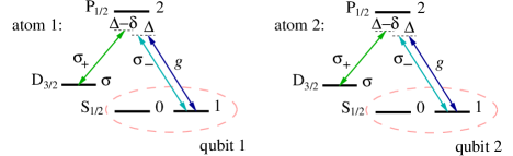
FIG. 1.: Level configuration for atom-cavity quantum computing with calcium ions showing the driving laser fields. The 2-$\sigma$ and the 2-1 transitions are activated by the laser radiations with amplitudes and polarizations given by $\Omega_{\sigma}$, $\sigma_{+}$ and $\Omega_{1}$, $\sigma_{-}$ respectively. Each qubit is obtained from two degenerate $S_{1/2}$ ground states of the same ion.

Let us denote the cavity photon annihilation and creation operator by $b$ and $b^{\dagger}$ while $\Delta$ is the detuning of the cavity with respect to the 2-1 transition of each atom. The occupation of the cavity is then given by $n=\langle b^{\dagger}b\rangle$. One laser drives the 2-1 transition of atom $i$ with Rabi frequency $\Omega^{(i)}_{1}$ and detuning $\Delta$; another one excites the 2-$\sigma$ transition with Rabi frequency $\Omega^{(i)}_{\sigma}$ and detuning $\Delta-\delta$. Going over to the interaction picture with respect to $H_{0}+\hbar\sum_{i}\,[\,\delta|\sigma\rangle_{ii}\langle\sigma|+\Delta\,|2\rangle_{ii}\langle 2|\,]$ where $H_{0}$ is the interaction-free Hamiltonian, one finds

$$H_{\rm I} = \sum_{i=1}^{2}\hbar g\,\big{[}\,|2\rangle_{ii}\langle 1|b+\text{H.c.}\,\big{]}$$ (5)

$$+{\textstyle{1\over 2}}\hbar\,\big{[}\,\Omega^{(i)}_{1}|1\rangle_{ii}\langle 2|+\Omega^{(i)}_{\sigma}|\sigma\rangle_{ii}\langle 2|+\text{H.c.}\,\big{]}$$

$$-\hbar\delta\,|\sigma\rangle_{ii}\langle\sigma|-\hbar\Delta\,|2\rangle_{ii}\langle 2|~{}.$$

The generation of a non-trivial time evolution requires in general a non-homogeneity in the Rabi frequencies of the laser fields with respect to the two atoms. Without loss of generality, we assume here that the Rabi frequencies of laser fields coupling to the same transition differ only in phase. In the following, entangling operations are realized by choosing

$$\Omega^{(1)}_{\sigma}=-\Omega^{(2)}_{\sigma}\equiv-\Omega_{\sigma}~{},$$ (6)

$$\Omega^{(1)}_{1}=-\Omega^{(2)}_{1}\equiv-\Omega_{1}/\sqrt{2}~{}.$$ (7)

These parameters can be implemented via common laser addressing by driving each transition with the same laser field and from an angle that produces a $\pi$ phase difference between atom 1 and 2.

One of the main sources for decoherence in atom-cavity setups is the leakage of photons through the cavity mirrors. However, the presence of high spontaneous decay rates does not necessarily lead to dissipation. As it has been shown in the past, the presence of a relatively strong atom-cavity coupling constant $g$ [32] can have the same effect as continuous measurements whether the cavity mode is empty or not. As a consequence, the time evolution of the system becomes restricted onto the decoherence-free states of the system with respect to cavity decay. In this Section, we exploit this effect and its consequences for the time evolution to significantly simplify the requirements for atom-cavity quantum computation.

In the next Section, Raman and STIRAP-like processes [30, 31] are introduced in order to minimize the population in the excited atomic state $|2\rangle$. Assuming that the population in level $2$ is negligible, the only condition that has to be fulfilled to avoid cavity decay is that the Rabi frequencies $\Omega_{1}$ and $\Omega_{\sigma}$ are sufficiently weak compared to the atom-cavity coupling constant $g$,

$$|\Omega_{1}|\,,\,\,|\Omega_{\sigma}|\ll g$$ (8)

This relation induces two different time scales in the system and allows for the calculation of the time evolution with the help of an adiabatic elimination. Figure 2 shows the most relevant transitions if the system is initially prepared in a qubit state with an empty cavity ($n=0$) and uses the abbreviations

$$|\alpha\rangle\equiv\big{(}\,|12\rangle-|21\rangle\,\big{)}/\sqrt{2}~{},$$ (9)

$$|A\rangle\equiv\big{(}\,|\sigma 1\rangle+|1\sigma\rangle\,\big{)}/\sqrt{2}~{},$$ (10)

$$|\tilde{\alpha}\rangle\equiv\big{(}\,|\sigma 2\rangle-|2\sigma\rangle\,\big{)}/\sqrt{2}~{},$$ (11)

$$|\tilde{A}\rangle\equiv\big{(}\,|\sigma 1\rangle-|1\sigma\rangle\,\big{)}/\sqrt{2}~{}.$$ (12)

Setting the amplitudes of all fast varying states equal to zero and using the Hamiltonian (5), one finds that the system evolves effectively according to the Hamiltonian

$$H_{\text{eff}} = \big{[}\,{\textstyle{1\over 2}}\hbar\,\big{(}\,\Omega_{1}\,|\alpha\rangle\langle 11|+\Omega_{\sigma}\,|\alpha\rangle\langle A|+\text{H.c.}\,\big{)}$$ (15)

$$-\hbar\delta\,|A\rangle\langle A|-\hbar\Delta\,|\alpha\rangle\langle\alpha|\,\big{]}\otimes|0_{\rm cav}\rangle\langle 0_{\rm cav}|~{}.$$

As expected for adiabatic processes, this Hamiltonian restricts the time evolution onto a subspace of slowly varying states, which is why the states $|\tilde{\alpha}\rangle$ and $|\tilde{A}\rangle$ are not present in Equation (15). The subspace of the slowly varying states includes, in addition to the ground states, only one state with population in the excited state $|2\rangle$. This state, $|\alpha\rangle|0_{\rm cav}\rangle$, is a zero eigenstate of the atom-cavity interaction.

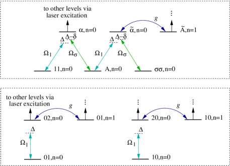
FIG. 2.: Level configuration showing the most relevant transitions for the initial qubit states $|11\rangle$, $|01\rangle$ and $|10\rangle$ in the presence of mechanisms (see Section III) that minimize the population in level 2. The presence of a strong cavity coupling constant $g$ prohibits a transfer of population between $|A\rangle$ and $|\sigma\sigma\rangle$. This does not effect the transition between $|11\rangle$ and $|A\rangle$. The atomic state $|00\rangle$ does not see any laser fields and does not change its amplitude in time.

Note that the Hamiltonian (15) indeed restricts the time evolution of the system onto its decoherence-free subspace with respect to cavity decay. A state belongs to this subspace if the resonator mode is in its vacuum state $|0_{\rm cav}\rangle$ and the atom-cavity interaction cannot transfer excitation from the atoms into the resonator. Hence, the decoherence-free subspace includes all ground states and the state $|\alpha\rangle|0_{\rm cav}\rangle$. They are exactly the slowly varying states of the system. Furthermore, the effective Hamiltonian can be written as

$$H_{\rm eff}=I\!\!P_{\rm DFS}\,H_{\rm laser}\,I\!\!P_{\rm DFS}~{},$$ (16)

where $I\!\!P_{\rm DFS}$ is the projector onto the decoherence-free subspace

$$I\!\!P_{\rm DFS}=\Big{[}|\alpha\rangle\langle\alpha|+\sum_{i,j=0,1,\sigma}|ij\rangle\langle ij|\Big{]}\otimes|0_{\rm cav}\rangle\langle 0_{\rm cav}|~{},$$ (17)

and $H_{\rm laser}$ is the laser term in (5). One way to interpret this is to state that condition (8) effectively induces continuous measurements whether the cavity field is empty or not [33]. As a consequence, entanglement can be generated between qubits via excitation of the maximally entangled state $|\alpha\rangle$.

In the event that condition (8) is not fulfilled, as in all realistic experiments, the above argumentation does not hold and corrections to the effective time evolution (15) have to be taken into account. To identify the evolution of the system more accurately, we use the quantum jump approach [34, 35, 36] which predicts the no-photon time evolution of the system with the help of the conditional, non-Hermitian Hamiltonian $H_{\rm cond}$. Given the initial state $|\psi\rangle$, the state of the system equals $U_{\rm cond}(T,0)\,|\psi\rangle/\|\cdot\|$ at time $T$ under the condition of no emission. For convenience, $H_{\rm cond}$ has been defined such that

$$P_{0}(T)=\|\,U_{\rm cond}(T,0)\,|\psi\rangle\,\|^{2}$$ (18)

is the probability for no photon in $(0,T)$. If photons are emitted, then the computation failed and has to be repeated. To some extent, this can be compensated by monitoring photon emissions with good detectors. Alternatively, quantum teleportation can be employed to perform a whole algorithm by selecting the successful gates [37].

Let us now consider a concrete example to see how well the elimination of cavity decay works. For the two four-level atoms in Figure 1 it is [20]

$$H_{\rm cond} = H_{\rm I}-{\textstyle{{\rm i}\over 2}}\hbar\kappa\,b^{\dagger}b-{\textstyle{{\rm i}\over 2}}\hbar\Gamma\,\sum_{i=1}^{2}|2\rangle_{ii}\langle 2|~{}.$$ (19)

Suppose that the system is initially prepared in $|01\rangle|0_{\rm cav}\rangle$ and a laser field is applied with $\Omega_{1}\neq 0$ that excites the 2-1 transition of both atoms for a significant time $T$. Equation (15) then implies the inhibition of any time evolution since $|01\rangle|0_{\rm cav}\rangle$ is a zero eigenstate of $H_{\rm eff}$. Indeed, the numerical solution of the time evolution given by the Hamiltonian (19) reveals that the final state coincides with the initial state of the system with fidelity $F\equiv 1$ under the condition of no photon emission in $(0,T)$. The success rate $P_{0}(T)$ as a function of $\Delta$ and $\Omega_{1}$ is shown in Figure 3. As expected, $P_{0}$ is the closer to one the smaller the Rabi frequency $\Omega_{1}$ and its size is widely independent from the detuning $\Delta$.

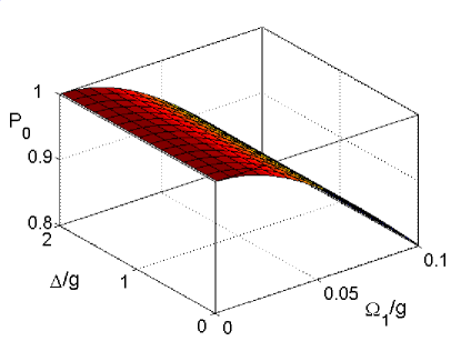
FIG. 3.: The success rate $P_{0}(T)$ as a function of the Rabi frequency $\Omega_{1}$ and the detuning $\Delta$ for the initial state $|01\rangle|0_{\rm cav}\rangle$, $\kappa=\Gamma=0.1\,g$, $\delta=0$ and $T=2000/g$. If one allows for a short transition time at the end of the operation for unwanted states to decay, then the final state of the system equals exactly the initial one.

III Elimination of atom decay and entangling operations

For optical cavities, the atom decay rate $\Gamma$ is in general of about the same size as the parameters $g$ and $\kappa$. We therefore still need to overcome the problem of spontaneous emission from the atoms in order to realize a coherent time evolution. This can be achieved by minimizing the population in level $2$ and keeping the system effectively in the ground states $|11\rangle|0_{\rm cav}\rangle$ and $|A\rangle|0_{\rm cav}\rangle$. To realize this we employ in the following Raman or STIRAP-like transitions [30, 31]. These are directly applicable since the relevant states comprise a $\Lambda$-type three-level configuration. Entanglement between the atoms is created by coupling $|11\rangle$ to the maximally entangled state $|A\rangle$.

A Entangling Raman transitions

One way to implement transitions without populating the excited state $|\alpha\rangle$ is to choose the detuning $\Delta$ much larger than the Rabi frequencies $\Omega_{1}$ and $\Omega_{\sigma}$,

—Ω_1—   ,   —Ω_σ— ≪Δ  (20)

This choice of parameters results in the realization of a Raman-like transition since the large detuning $\Delta$ introduces an additional time scale in the time evolution (15). Adiabatically eliminating the excited state $|\alpha\rangle$ reveals that the system is effectively governed by the Hamiltonian

$$H_{\rm eff} = {\textstyle{1\over 2}}\hbar\Omega\,\big{[}\,|11\rangle\langle A|+\text{H.c.}\,\big{]}$$ (23)

$$-\hbar\Delta_{11}\,|11\rangle\langle 11|-\hbar\Delta_{A}\,|A\rangle\langle A|$$

with the abbreviations

$$\Omega\equiv{\Omega_{1}\Omega_{\sigma}^{*}\over 2\Delta}~{},~{}\Delta_{11}\equiv-{|\Omega_{1}|^{2}\over 4\Delta}~{},~{}\Delta_{A}\equiv\delta-{|\Omega_{\sigma}|^{2}\over 4\Delta}~{}.$$ (24)

Solving the time evolution for the case where the lasers are turned on for a period $T$ with constant amplitude yields

$$U_{\rm eff}(T,0) = \exp\left({\textstyle{{\rm i}\over 2}}(\Delta_{11}+\Delta_{A})T\right)\left[\,\left(\,\cos{\textstyle{KT\over 2}}+{\textstyle{{\rm i}(\Delta_{11}-\Delta_{A})\over K}}\,\sin{\textstyle{KT\over 2}}\right)|11\rangle\langle 11|\right.$$ (26)

$$\left.-{\textstyle{\Omega\over K}}\sin{\textstyle{KT\over 2}}\,\big{(}\,|11\rangle\langle A|+|A\rangle\langle 11|\,\big{)}+\left(\,\cos{\textstyle{KT\over 2}}-{\textstyle{{\rm i}(\Delta_{11}-\Delta_{A})\over K}}\,\sin{\textstyle{KT\over 2}}\right)|A\rangle\langle A|\,\right]~{},$$

where

$$K\equiv\left(|\Omega|^{2}+(\Delta_{11}-\Delta_{A})^{2}\right)^{1/2}$$ (27)

plays the role of a Rabi frequency. As the evolution (26) can be used to create entanglement, we call it an entangling Raman (E-Raman) transition.

In order to see how well the elimination of the dissipative states works, let us consider as an example the preparation of the maximally entangled state $|A\rangle$. If the atoms are initially in $|11\rangle$, this can be achieved by applying a laser pulses of length $T=\pi/K=2\pi\Delta|\Omega_{1}|^{2}$ with $\delta=0$ and $\Omega_{\sigma}=\Omega_{1}$. Figures 4 and 5 present the fidelity $F$ and success rate $P_{0}$, respectively, of this entangling operation as a function of the Rabi frequency $\Omega_{1}$ and the detuning $\Delta$. They result from a numerical integration of the time evolution with the full Hamiltonian (19).

In particular for $\kappa=\Gamma=0.1\,g$, the fidelity of the final state can be as high as 0.993 if one chooses $\Omega_{1}=0.01\,g$ and $\Delta=1.357\,g$ and allows the success probability to be as high as $P_{0}=0.857$. Higher fidelities can only be obtained in the presence of smaller decay rates. In general one can improve the success rate $P_{0}$ by a few percent by increasing the detuning $\Delta$ and by sacrificing an error from the maximal fidelity of the order of $10^{-3}$. While the fidelity exhibits a maximum as a function of $\Delta$, the success probability increases monotonically with $\Delta$. For large detunings, the adiabatic elimination of the cavity mode is no longer efficient (see Figure 2) resulting in the reduction of $F$. Varying the Rabi frequency gives larger fidelities for smaller $\Omega_{1}$ since the adiabatic elimination of cavity excitation as well as the elimination of $|\alpha\rangle$ becomes more efficient. However, the smaller $\Omega_{1}$ the larger the operation time $T$ of the entangling evolution.

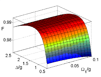
FIG. 4.: The fidelity $F$ for the preparation of the maximally entangled state $|A\rangle$ given the initial state $|11\rangle$ as functions of the Rabi frequency $\Omega_{1}$ and the detuning $\Delta$ for $\Omega_{\sigma}=\Omega_{1}$, $\Gamma=\kappa=0.1\,g$ and $\delta=0$.

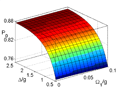
FIG. 5.: The success rate $P_{0}$ for the preparation of the maximally entangled state $|A\rangle$ for the same parameters as in Figure 4.

B Entangling STIRAP processes

Another way to transfer population between the ground states $|11\rangle$ and $|A\rangle$ without ever populating the excited state $|\alpha\rangle$ is to employ a STIRAP-like process [30, 31]. As this is an entangling process we can call it an entangling STIRAP (E-STIRAP) transition. To see how the suppression of spontaneous emission from the atoms works in this case let us consider again the effective Hamiltonian (15) and note that its eigenvalues for $\delta\ll\Delta$ are

$$E_{0}=0~{},~{}E_{\pm}={\textstyle{1\over 2}}(-\Delta\pm\sqrt{|\Omega_{\sigma}|^{2}+|\Omega_{1}|^{2}+\Delta^{2}})~{}.$$ (28)

For convenience, we now introduce the interaction picture with respect to the Hamiltonian $H_{0}=-\hbar\delta|A\rangle\langle A|$. Within that picture, the eigenvectors of the effective Hamiltonian become time dependent and the dark state of the system equals

$$|E_{0}\rangle\equiv{1\over\sqrt{|\Omega_{\sigma}|^{2}+|\Omega_{1}|^{2}}}\,\big{(}\Omega_{\sigma}|11\rangle-{\rm e}^{-{\rm i}\delta t}\,\Omega_{1}|A\rangle\big{)}~{}.$$ (29)

The other two eigenstates $|E_{\pm}\rangle$ occupy the antisymmetric state $|\alpha\rangle$ and hence possess population in the excited atomic state $|2\rangle$.

Spontaneous emission from the atoms can therefore be avoided if the system remains constantly in the dark state $|E_{0}\rangle$. Nevertheless, a nontrivial entangling time evolution between the ground states $|11\rangle$ and $|A\rangle$ can be induced, by varying the laser amplitudes $\Omega_{1}$ and $\Omega_{\sigma}$ in time. If this happens slow compared to the time scale given by the eigenvalues $E_{\pm}$, no population is transferred into the eigenstates $|E_{\pm}\rangle$. Assuming adiabaticity, the system follows the changing parameters and remains in the dark state. The fact that $|E_{0}\rangle$ incorporates a time dependent phase factor can be used to induce a certain phase on the final state $|A\rangle$ by choosing the small laser detuning $\delta$ appropriately.

In the following we assume $\Delta=0$ since this maximizes the energy distance between $|E_{0}\rangle$ and its nearest eigenstate. For convenience, we also consider the case where $\Omega_{1}$ and $\Omega_{\sigma}$ are real and define $\tan\theta\equiv\Omega_{1}/\Omega_{\sigma}$ and $\phi\equiv-\delta t$. The eigenstate corresponding to the zero eigenvalue then takes the familiar form

$$|E_{0}\rangle=\cos\theta\,|11\rangle-{\rm e}^{{\rm i}\phi}\sin\theta\,|A\rangle~{}.$$ (30)

The adiabatic condition is satisfied if

—˙θ—   ,    —˙ϕ— ≪Ω_σ^2 + Ω_1^2 (31)

If the time dependence of $\theta$ and $\phi$ is indeed such that the initial state of the system coincides with the dark state $|E_{0}(0)\rangle$, the effective evolution along a path $C$ in the $(\theta,\phi)$ parameter space can easily be calculated. As a consequence of the adiabatic theorem, the effective evolution is diagonal with respect to the basis given by the eigenvectors $|E_{0}\rangle$ and $|E_{\pm}\rangle$. Especially for the case where $\theta(0)=0$ and with respect to the basis states $|E_{0}(0)\rangle$, $|E_{+}(0)\rangle$ and $|E_{-}(0)\rangle$, the effective time evolution of the system can be written as

$$U_{\rm eff}(T,0)=R(\theta,\phi)\left(\begin{array}[]{ccc}{\rm e}^{{\rm i}\varphi_{0}}&0&0\\ 0&{\rm e}^{{\rm i}\varphi_{+}}&0\\ 0&0&{\rm e}^{{\rm i}\varphi_{-}}\end{array}\right)$$ (32)

with $\theta=\theta(T)$, $\phi=\phi(T)$ and

$$R(\theta,\phi)={\textstyle{1\over 2}}\times$$ (33)

$$\left(\begin{array}[]{ccc}2\cos\theta&\sqrt{2}\sin\theta&\sqrt{2}\sin\theta\\ -\sqrt{2}{\rm e}^{{\rm i}\phi}\sin\theta&(1+{\rm e}^{{\rm i}\phi}\cos\theta)&-(1-{\rm e}^{{\rm i}\phi}\cos\theta)\\ \sqrt{2}{\rm e}^{{\rm i}\phi}\sin\theta&(1-{\rm e}^{{\rm i}\phi}\cos\theta)&-(1+{\rm e}^{{\rm i}\phi}\cos\theta)\end{array}\right)~{}\!\!.$$ (37)

The phases $\varphi_{i}\equiv\varphi^{\text{d}}_{i}+\varphi^{\text{g}}_{i}$ ($i=0,\,\pm$) are in general the sum of a dynamical and a geometrical phase with

$$\varphi^{\text{d}}_{0}=0~{},~{}\varphi^{\text{d}}_{+}=-\varphi^{\text{d}}_{-}=-{\textstyle{1\over 2}}\int_{0}^{T}\sqrt{\Omega_{1}^{2}+\Omega_{\sigma}^{2}}\,{\rm d}t$$ (38)

while the geometrical phases equal

$$\varphi^{\text{g}}_{0}=\oint_{C}\sin^{2}\theta\,{\rm d}\phi~{},~{}\varphi^{\text{g}}_{+}=\varphi^{\text{g}}_{-}={\textstyle{1\over 2}}\oint_{C}\cos^{2}\theta\,{\rm d}\phi$$ (39)

for a closed circular loop $C$.

As an example, let us consider the case where the initial state $|11\rangle$ is transferred into the maximally entangled state $|A\rangle$. This can be achieved by varying the Rabi frequencies $\Omega_{1}$ and $\Omega_{\sigma}$ slowly in a so-called counterintuitive pulse sequence. Figure 6 and 7 show the result of a numerical solution of the corresponding time evolution taking the full Hamiltonian (19) into account. In particular, we calculated the fidelity and the success of the scheme as a function of the maximum laser amplitude $\Omega$ and the frequency $\omega$ for $\Delta=\delta=0$, $\kappa=\Gamma=0.1\,g$ and

$$\Omega_{\sigma}(t)=\left\{\begin{array}[]{cl}\Omega\,\sin\omega t\,,&{\rm for}~{}t\in\big{(}0,{\textstyle{2\over 3}}T\big{)}\\[5.69046pt] 0\,,&{\rm for}~{}t\in\big{(}{\textstyle{2\over 3}}T,T\big{)}\end{array}\right.$$ (40)

and

$$\Omega_{1}(t)=\left\{\begin{array}[]{cl}0\,,&{\rm for}~{}t\in\big{(}0,{\textstyle{1\over 3}}T\big{)}\\[5.69046pt] \Omega\,\sin\omega\big{(}t-{\textstyle{1\over 3}T}\big{)}\,,&{\rm for}~{}t\in\big{(}{\textstyle{1\over 3}}T,T\big{)}\end{array}\right.$$ (41)

with the total operation time $T=3\pi/(2\omega)$.

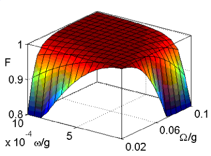
FIG. 6.: The fidelity $F$ for the preparation of the maximally entangled state $|A\rangle$ as a function of the maximum Rabi frequency $\Omega$ and frequency $\omega$ for $\Delta=\delta=0$ and $\kappa=\Gamma=0.1\,g$.

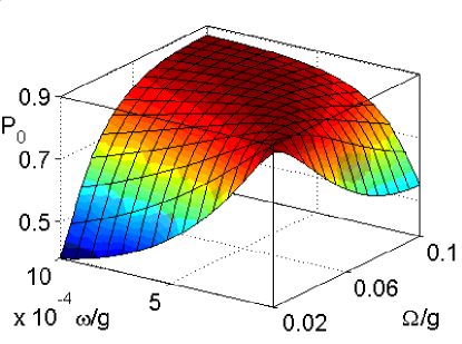
FIG. 7.: The success rate $P_{0}$ for the proposed entangled state preparation scheme for the same parameters as in Figure 6.

In contrast to E-Raman processes, the fidelity $F$ of the final state can, in principle, be arbitrarily close to one independent of the size of the spontaneous decay rates $\kappa$ and $\Gamma$. For example, for $\Omega=0.02\,g$ and $\omega=4\cdot 10^{-5}\,g$ the fidelity becomes $F=0.998$ and corresponds to the success rate $P_{0}=0.876$ which is still within acceptable limits. In general, a large $\Omega$ leads to the population of the excited state $|2\rangle$ which might result in the emission of a photon with rate $\Gamma$ or in the population of the cavity mode followed by the leakage of a photon through the cavity mirrors. As a result, $F$ and $P_{0}$ decrease for increasing laser amplitudes $\Omega$. On the other hand, for very weak Rabi frequencies $(\Omega\approx 0)$ the fidelity and the success rate increase as $\omega$ decreases which results in a longer operation time $T$. This is in agreement with condition (31) which implies that the adiabatic evolution is more successful for slower evolutions. Nevertheless, the success rate $P_{0}$ cannot be increased arbitrarily. The reason is that very long operation times unavoidably lead to the population of the cavity mode in the presence of a finite value for $\Omega$ and the elimination of cavity decay does no longer hold.

IV Decoherence-free dynamical and geometrical phase gates

In this Section we employ the decoherence-free E-Raman and E-STIRAP processes introduced in the last Section for the realization of two-qubit quantum gate operations. In particular, we consider the implementation of the controlled phase gate

$$CP={\text{diag}}\,\big{(}1,1,1,{\rm e}^{{\rm i}\varphi}\big{)}~{},$$ (42)

where the qubit state $|11\rangle$ collects the phase $\varphi$ while the other qubit states remain unaffected. This gate constitutes, together with a general single-qubit rotation, a universal set of gates and allows for the implementation of any desired unitary time evolution. Attention is paid to their stability against fluctuations of most system parameters and we analyze in detail the efficiency of various processes.

A Raman-based Dynamical Phase Gates

Let us begin with the description of a possible implementation of (42) with the help of the E-Raman process introduced in Section IIIA. From Equation (26) one sees that an applied laser pulse of length $T$ evolves the initial state $|11\rangle$ according to

$$U_{\text{eff}}(T,0)|11\rangle = \exp\left({\textstyle{{\rm i}\over 2}}(\Delta_{11}+\Delta_{A})T\right)\times$$ (45)

$$\Big{[}\,\Big{(}\cos{\textstyle{KT\over 2}}+{\rm i}{\textstyle{\Delta_{11}-\Delta_{A}\over K}}\sin{\textstyle{KT\over 2}}\Big{)}|11\rangle-\textstyle{\Omega\over K}\sin{\textstyle{KT\over 2}}|A\rangle\,\Big{]}~{},$$

while the amplitudes of the qubit states $|00\rangle$, $|01\rangle$ and $|10\rangle$ do not change in time. The desired phase gate (42) can therefore be realized in the minimal time if one chooses

$$T={2\pi/K}~{}.$$ (47)

For this parameter choice, the sine term in (LABEL:11) vanishes and the cosine term equals $-1$ giving finally

$$\varphi=\pi+{\textstyle{1\over 2}}(\Delta_{11}+\Delta_{A})T~{}.$$ (48)

Again, the phase $\varphi$ can be controlled by adjusting the size of the detuning $\delta$. Especially, for

$$\delta={\textstyle{1\over 4\Delta}}\big{(}|\Omega_{1}|^{2}+|\Omega_{\sigma}|^{2}\big{)}$$ (49)

one obtains $\varphi=\pi$ and the amplitude of the state $|11\rangle$ accumulates a minus sign. This particular evolution is illustrated in Figure 8 using a Bloch’s sphere representation. Note that the condition of timing the evolution such that the sine term becomes zero, is robust against first order timing errors in $T$ due to the behaviour of the sine function around $\pi$.

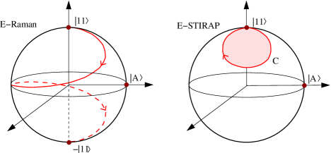
FIG. 8.: The E-Raman and E-STIRAP evolutions depicted on the Bloch sphere. In the E-Raman evolution, the generation of the phase factor in front of $|11\rangle$ is explicitly shown. In the E-STIRAP evolution, the acquired phase relates to the solid angle spanned by the path $C$ on the sphere.

To minimize the experimental effort for the realization of the phase gate (42), one should notice that a non-trivial E-Raman transition can also be induced using only one laser field coupling to the 1-2 transition of each atom. Indeed, for $\Delta_{A}=0$ and the laser pulse duration $T=\pi/K$, Equation (LABEL:11) yields

$$U_{\text{eff}}(T,0)|11\rangle=-\exp\big{(}{\rm i}\Delta_{11}T\big{)}\,|11\rangle~{}.$$ (50)

For this case, Figure 2 shows that the initial state $|11\rangle$ couples only to the excited state $|\alpha\rangle$ via the applied heavily detuned laser field. To see that the phase operation (50) is robust against fluctuations of $\Omega_{1}$, we now consider the Rabi frequency being time dependent. In this case the phase accumulated by the initial state $|11\rangle$ becomes $\varphi=\pi+\int_{0}^{T}\Delta_{11}{\rm d}t$. This clearly shows that statistical perturbations of $\Omega_{1}$ average out due to dependence of the acquired phase on the integral over $\Delta_{11}$ along $(0,T)$.

B STIRAP-based Geometrical Phase gate

Another possibility to implement the controlled two-quit phase gate (42) is provided by the E-STIRAP process. Let us first consider the case of the generation of a dynamical phase as in [20]. To do so we vary $\theta$ from zero to $\pi$, then apply a $2\pi$ pulse to transform the state $|\sigma\rangle$ to $-|\sigma\rangle$ for both atoms and then reduce $\theta$ back to zero. At the end of this time evolution, the state $|11\rangle$ acquires an overall minus sign, while the other qubit states $|00\rangle$, $|01\rangle$ and $|10\rangle$ remain unchanged. The result is the conditional phase gate with $\varphi=\pi$.

Alternatively, a geometrical phase can be generated by continuously varying the parameters $\theta$ and $\phi$ in a cyclic fashion [38, 39]. Starting from $\theta=0$ one can perform a cyclic adiabatic evolution on the $(\theta,\phi)$ plane along a loop $C$. As predicted by Equations (32)-(39), the qubit state $|11\rangle$ then acquires the geometrical phase

$$\varphi=\varphi^{\rm g}_{0}=\oint_{C}\sin^{2}\theta\,{\rm d}\phi$$ (51)

while the dynamical phase $\varphi^{\rm d}_{0}$ is identically zero. The concrete size of $\varphi$, which characterizes the phase gate (42), depends therefore only on the solid angle spanned by the path $C$ on the Bloch sphere (see Figure 8). Hence it is very robust against statistical fluctuations of the Rabi frequencies of the applied laser fields and it is independent of the total gate operation time.

Let us now consider a concrete laser configuration, where the laser field $\Omega_{\sigma}$ is turned on and kept constant. To perform a non-trivial loop in the control parameter space $(\theta,\phi)$ starting from the $(0,0)$ point we proceed as follows. As described in Section III B, a non-zero detuning $\delta$ results in the accumulation of a phase $\phi=-\delta t$ when we introduce a non zero value for $\theta$. Let us consider the simple case where

$$\theta=\arctan\,(x)~{}~{}{\rm with}~{}~{}x\equiv\Omega_{1}/\Omega_{\sigma}~{},$$ (52)

changes from zero to a non-zero value. More concretely, we increase and decrease $\Omega_{1}$ by linear ramps such that

$$x(t)=\left\{\begin{array}[]{cl}\alpha t\,,&{\rm for}~{}t\in\big{(}0,{\textstyle{1\over 2}}T\big{)}\\[5.69046pt] \alpha(T-t)\,,&{\rm for}~{}t\in\big{(}{\textstyle{1\over 2}}T,T\big{)}\end{array}\right.$$ (53)

or by a sine ramp given by

$$x(t)=x_{\text{max}}\,\sin\beta t$$ (54)

with $t\in(0,\pi/\beta)$. For those two cases one can easily derive the geometrical phases as functions of the experimental control parameters $T$, $\alpha$, $x_{\text{max}}$ and $\beta$ and we present the results in Figure 9.

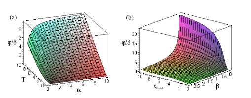
FIG. 9.: The resulting geometrical phase $\varphi^{\text{g}}/\delta$ produced (a) by a linear ramp and (b) by a sine ramp. The produced geometrical phases are largely independent of the control parameters $\alpha$ or $x_{\text{max}}$ respectively. $\alpha$ and $\beta$ are depicted in inverse time units, while $x_{\text{max}}$ is dimensionless.

From the plots we see that the accumulated geometrical phase $\varphi$ is, as expected, widely independent on the size of $\alpha$ or $x_{\text{max}}$ giving the resilience of the proposed E-STIRAP process from control errors, especially from the exact value of the laser amplitudes or their time derivatives. This independence of $\varphi$ makes the proposed quantum gate implementation an attractive candidate for experiments where the exact control of all laser parameters is not possible. In addition, it is experimentally appealing to construct a setup where the two employed laser fields can be produced from the same source, separated in two by a beam splitter and having the ratio $\Omega_{1}/\Omega_{\sigma}$ modulated e.g. by an Acousto-Optical Modulator (AOM). With this setup, the ratio is also resilient to the fluctuations of the amplitude of the initial laser beam.

V Conclusions

In this paper, we discussed in detail concrete proposals for the realization of universal two-qubit phase gates for quantum computing in atom-cavity setups. The atoms (or ions) are trapped at fixed positions inside an optical cavity and each qubit is obtained from two stable ground states of the same atom. To activate a time evolution, two laser fields are applied simultaneously inducing transitions in an effectively $\Lambda$-like system. In order to minimize the experimental effort, we seek quantum computing schemes that are as simple as possible in terms of resources. The quantum gate implementations proposed here do not require individual addressing of the atoms and can be realized, essentially, within one step. In particular, we considered the case where the atom-cavity coupling constant $g$ is only one order of magnitude larger than each of the spontaneous decay rates of the system and we assumed $g^{2}=100\,\kappa\Gamma$.

To avoid dissipation, we populate only the ground state of the system including all stable ground states of the atoms while the cavity is in its vacuum state. Nevertheless, an interaction between qubits can take place via virtual population of the cavity mode and excited atomic levels. We first eliminated the possibility of leakage of photons through the cavity mirrors. This was achieved by choosing the parameters such that adiabaticity restricts the time evolution of the system effectively onto a decoherence-free subspace with respect to cavity decay that includes highly entangled atomic states. Using these states for the implementation of Raman and STIRAP-like evolutions, entanglement can be created between the ground states of the atoms.

Comparing the E-Raman and E-STIRAP procedures we see that they give in general similar fidelities and success rates, with E-STIRAP having a slight advantage. Their control procedures are quite different in both cases, providing a flexibility to adapt the proposed scheme to different experimental setups. The main conceptual as well as practical difference appears when we produce the entangling phase gates. As it is seen in Figure 8 the phase produced by the E-Raman transition on the state $|11\rangle$ is given explicitly by the evolution of this state from the north to the south pole of the Bloch sphere. In contrast, with the E-STIRAP procedure initial population in the $|11\rangle$ state circulates along a closed path and returns exactly to the initial point. Nevertheless, at the end the state $|11\rangle$ acquires a geometrical phase.

The idea of using measurements on ancilla states, like the measurements on the cavity mode considered in this paper, leads to a realm of new possibilities for quantum computing. A recent example is the linear optics scheme by Knill et al. [37] where photons become entangled without ever having to interact. As long as the measurements on the ancilla state do not reveal any information about the qubits, they induce a unitary time evolution between them which can then be used to implement universal gate operations [40]. In contrast to other schemes, the gate success rate for atom-cavity quantum computing can, at least in principle, be arbitrarily close to one since the measurements are performed almost continuously. This allows to utilize the quantum Zeno effect [18] which assures that transitions in unwanted states are strongly inhibited.

The proposed schemes exhibit stability against fluctuations of most system parameters. The presented dynamical and geometrical phases are obtained by a time evolution that does not dependent on the exact value of the external control parameters. Using E-Raman or E-STIRAP processes, we enjoy the experimental advantages, such as, independence of the final state on the exact intermediate value of the laser field amplitude. Gates are constructed dynamically as well as geometrically in order to take advantage of the additional fault-tolerant features of geometrical quantum computation [41]. Recently, many attempts have been made in exploring the decoherence characteristics of geometrical phases [42, 43]. Whether they are advantageous over equivalent dynamical evolutions depends on the employed physical system. In contrast to this, we presented here evolutions that are intrinsically decoherence-free and naturally allow the generation of entangling dynamical as well as geometrical phases with simple control pictures.

Acknowledgements. This work was supported in part by the European Union and the EPSRC. A.B. thanks the Royal Society for a James Ellis University Research Fellowship.

REFERENCES

- [1] M. O. Scully and K. Drühl, Phys. Rev. A 25, 2208 (1982); U. Eichmann, J. C. Bergquist, J. J. Bollinger, J. M. Gilligan, W. M. Itano, D. J. Wineland, and M. G. Raizen, Phys. Rev. Lett. 70 2359 (1993).
- [2] Z. Hradil, R. Myska, J. Perina, M. Zawisky, Y. Hasegawa, and H. Rauch, Phys. Rev. Lett. 76, 4295 (1996).
- [3] D. Bouwmeester, G. P. Karman, C. A. Schrama, J. P. Woerdman, Phys. Rev. A 53, 985 (1996).
- [4] B. Brezger, L. Hackermüller, S. Uttenthaler, J. Petschinka, M. Arndt, and A. Zeilinger, Phys. Rev. Lett. 88, 100404 (2002).
- [5] M. Berry, I. Marzoli, and W. Schleich, Phys. World 14, 39 (2001).
- [6] J. P. Dowling, Phys. Rev. A 57, 4736 (1998).
- [7] J. P. Dowling and G. J. Milburn, Quantum Technology: The Second Quantum Revolution, quant-ph/0206091.
- [8] C. H. Bennett and D. P. DiVincenzo, Nature 404, 247 (2000).
- [9] M. Hennrich, T. Legero, A. Kuhn, and G. Rempe, Phys. Rev. Lett. 85, 4872 (2000); A. Kuhn, M. Hennrich, and G. Rempe, Phys. Rev. Lett. 89, 067901 (2002).
- [10] J. McKeever, A. Boca, A. D. Boozer, J. R. Buck, and H. J. Kimble, Nature 425, 268 (2003).
- [11] J. A. Sauer, K. M. Fortier, M. S. Chang, C. D. Hamley, and M. S. Chapman, Cavity QED with optically transported atoms, quant-ph/0309052.
- [12] G. R. Guthöhrlein, M. Keller, K. Hayasaka, W. Lange, and H. Walther, Nature 414, 49 (2001).
- [13] C. Schön and J. I. Cirac, Phys. Rev. A 67, 043813 (2003).
- [14] T. Fischer, P. Maunz, P. W. H. Pinkse, T. Puppe, and G. Rempe, Phys. Rev. Lett. 88, 163002 (2002).
- [15] P. Horak, B. G. Klappauf, A. Haase, R. Folman, J. Schmiedmayer, P. Domokos, and E. A. Hinds, Phys. Rev. A 67, 043806 (2003).
- [16] T. Pellizzari, S. A. Gardiner, J. I. Cirac, and P. Zoller, Phys. Rev. Lett. 75, 3788 (1995).
- [17] P. Domokos, J. M. Raimond, M. Brune, and S. Haroche, Phys. Rev. A 52, 3554 (1995).
- [18] A. Beige, D. Braun, B. Tregenna, and P. L. Knight, Phys. Rev. Lett. 85, 1762 (2000); B. Tregenna, A. Beige, and P. L. Knight, Phys. Rev. A 65, 032305 (2002).
- [19] S.-B. Zheng and G.-C. Guo, Phys. Rev. Lett. 85, 2392 (2000).
- [20] J. Pachos and H. Walther, Phys. Rev. Lett. 89, 187903 (2002).
- [21] E. Jané, M. B. Plenio, and D. Jonathan, Phys. Rev. A 65, 050302 (2002).
- [22] A. Recati, T. Calarco, P. Zanardi, J. I. Cirac, and P. Zoller, Phys. Rev. A 66, 032309 (2002).
- [23] L. You, X. X. Yi, and X. H. Su, Phys. Rev. A 67, 032308 (2003); X. X. Yi, X. H. Su, and L. You, Phys. Rev. Lett. 90, 097902 (2003).
- [24] A. S. Sørensen and K. Mølmer, Phys. Rev. Lett. 91, 097905 (2003).
- [25] M. V. Berry, Proc. R. Soc. London Ser. A 392, 45 (1984).
- [26] G. Palma, K.-A. Suominen, and A. Ekert, Proc. Roy. Soc. London Ser. A 452, 567 (1996).
- [27] P. Zanardi and M. Rasetti, Phys. Rev. Lett. 79, 3306 (1997).
- [28] D. A. Lidar, I. L. Chuang, and K. B. Whaley, Phys. Rev. Lett. 81, 2594 (1998).
- [29] A. Beige, D. Braun, and P. L. Knight, New J. Phys. 2, 22 (2000).
- [30] J. Oreg, F. T. Hioe, and J. H. Eberly, Phys. Rev. A 29, 690 (1984).
- [31] K. Bergmann, H. Theuer, and B. W. Shore, Rev. Mod. Phys. 70, 1003 (1998); N. V. Vitanov, T. Halfmann, B. W. Shore, and K. Bergmann, Annu. Rev. Phys. Chem. 52, 763 (2001).
- [32] C. Marr, A. Beige, and G. Rempe, Phys. Rev. A 68, 033817 (2003).
- [33] For a detailed description of quantum computing using dissipation see A. Beige, Phys. Rev. A (in press), Section II; quant-ph/0304168.
- [34] G. C. Hegerfeldt and T. S. Wilser, in Classical and Quantum Systems, Proceedings of the Second International Wigner Symposium, July 1991, edited by H. D. Doebner, W. Scherer, and F. Schroeck (World Scientific, Singapore, 1992), p. 104; G. C. Hegerfeldt and D. G. Sondermann, Quant. Semiclass. Opt. 8, 121 (1996).
- [35] J. Dalibard, Y. Castin, and K. Mølmer, Phys. Rev. Lett. 68, 580 (1992).
- [36] H. Carmichael, An Open Systems Approach to Quantum Optics, Lecture Notes in Physics, Vol. 18 (Springer, Berlin, 1993).
- [37] E. Knill, R. Laflamme, and G. J. Milburn, Nature 409, 46 (2001).
- [38] P. Zanardi and M. Rasetti, Phys. Lett. A 264, 94 (1999); J. Pachos, “Quantum Computation by Geometrical Means”, published in the AMS Contemporary Math Series volume entitled “Quantum Computation & Quantum Information Science”.
- [39] D. Bouwmeester, G. P. Karman, N. H. Dekker, C. A. Schramm, and J. P. Woerdman, J. Mod. Opt. 43, 2087 (1996).
- [40] G. G. Lapaire, P. Kok, J. P. Dowling, and J. E. Sipe, Conditional linear-optical measurement schemes generate effective photon nonlinearities, quant-ph/0305152.
- [41] D. Ellinas and J. Pachos, Phys. Rev. A 64, 022310 (2001).
- [42] A. Nazir, T. P. Spiller, and W. J. Munro, Phys. Rev. A 65, 042303 (2002).
- [43] A. Carollo, I. Fuentes-Guridi, M. F. Santos, and V. Vedral, Phys. Rev. Lett. 90, 160402 (2003).