Wave Equations With Energy Dependent Potentials.

Abstract :

We study wave equations with energy dependent potentials. Simple analytical models are found useful to illustrate difficulties encountered with the calculation and interpretation of observables. A formal analysis shows under which conditions such equations can be handled as evolution equation of quantum theory with an energy dependent potential. Once these conditions are met, such theory can be transformed into ordinary quantum theory.

1 Introduction

Wave equations with energy dependent potentials have been known for long time. They appeared along with the Klein-Gordon equation for a particle in an external electromagnetic field [1]. In non-relativistic quantum mechanics, they arise from momentum dependent interactions, as shown by Green [2]. The Pauli-Schrödinger equation represents another example [3, 4]. A Hilbert space formulation of the relativistic quantum mechanical two-body problem was studied by Rizov et al [5]. These authors derived an algorithm for a perturbative calculation of the energy eigenvalues in the case of a general energy dependent quasipotential. The problem was first solved for the particular case of the relativistic harmonic oscillator [6].

In recent years, numerous works have been devoted to the Hamiltonian formulation of relativistic quantum mechanics in connection with the manifestly covariant formalism with constraints [7, 8]. The main advantage of this approach is to allow the proper separation of relative and center-of-mass coordinates in few-body and even in many-body problem, and thus to eliminate spurious degrees of freedom. The constraints impose restrictions to the potentials to be physically acceptable. As a result, the potentials become energy dependent. Links with field theory have been developed by taking the Bethe-Salpeter equation as a starting point. This makes the approach a challenging one. A typical application of the manifestly covariant formalism is a calculation of spectra of baryonic atoms. Work along this line has been carried out by Mourad and Sazdjian [9]. In particular, they have derived two-fermion relativistic wave equations, which acquire the form of Pauli-Schrödinger equations.

The presence of the energy dependent potential in a wave equation has several non-trivial implications. The most obvious one is the modification of the scalar product, necessary to ensure the conservation of the norm [10]. However, the modification of the scalar product itself is not sufficient to justify the use of the common rules of quantum mechanics. In the next section, we illustrate the aforementioned difficulties on a few simple models, admitting analytical solution.

Of course, testing formulas on a particular model does not guarantee their general validity in more realistic, physical systems. In section 3, we therefore analyze formal aspects and demonstrate under what circumstances a wave equation with an energy dependent potential corresponds to an acceptable quantum theory. We show that in such a case the wave equation can be transformed into an equivalent ordinary Schrödinger equation with a local, momentum dependent potential. Implications of the formal treatment are illustrated in section 4 and conclusions are drawn in the last section.

2 A toy model.

2.1 Generalities.

For the sake of simplicity, the toy model is constructed in the 1-dimensional space.

The starting point is the time dependent wave equation

$$i\frac{\partial}{\partial t}\Psi(x,t)=[-\frac{1}{2}\frac{\partial^{2}}{\partial x^{2}}+V(x,i\frac{\partial}{\partial t})]\Psi(x,t)\ ,$$ (1)

where $V(x,i\frac{\partial}{\partial t})$ denotes a real function of 2 variables. Setting $\Psi(x,t)=e^{-iEt}\psi(x)$ yields

$$H\psi(x)=[-\frac{1}{2}\frac{\partial^{2}}{\partial x^{2}}+V(x,E)]\psi(x)=E\psi(x)\ .$$ (2)

The first modification of the usual rules of quantum mechanics concerns the scalar product. This question has been studied by many authors in the one- and two-particle relativistic quantum mechanics (see Sazdjian [7] and references therein). For completeness, we present a brief sketch in the 1-dimensional case :

Consider two solutions of energies $E$ and $E^{\prime}$

$$\Phi_{\epsilon}(x,t)=e^{-i(E-i\epsilon)t}\Phi(x),\ \ \ {\rm and}\ \ \ \ \Psi_{\epsilon}(x,t)=e^{-i(E^{\prime}-i\epsilon)t}\Psi(x),$$ (3)

with $\epsilon\rightarrow 0$. The usual continuity equation reads

$$\frac{\partial}{\partial t}P=-\frac{\partial}{\partial x}j\ ,$$ (4)

where

$$P=\Psi^{*}_{\epsilon}(x,t)\Phi_{\epsilon}(x,t)\ \ ;\ \ j=-i\Big{[}\Psi^{*}_{\epsilon}(x,t)(\frac{\partial}{\partial x}\Phi_{\epsilon}(x,t))-(\frac{\partial}{\partial x}\Psi^{*}_{\epsilon}(x,t))\Phi_{\epsilon}(x,t)\Big{]}\ .$$

In the case of energy dependent potential, in order to fulfill the continuity equation, a term

$$\frac{\partial}{\partial t}P_{a}=i\Psi_{\epsilon}^{*}(x,t)[V(x,E)-V(x,E^{\prime})]\Phi_{\epsilon}(x,t)\$$ (5)

has to be added to the left hand side of Eq. (4). After integration, Eq. (5) yields

$$P_{a}=-\Psi_{\epsilon}^{*}(x,t)\Big{[}\frac{V(x,E^{\prime})-V(x,E)}{E^{\prime}-E}\Big{]}\Phi_{\epsilon}(x,t)\ ,$$ (6)

as $\epsilon\rightarrow 0$. As a result, in the limit $E^{\prime}\rightarrow E$, the scalar product (the norm) is given by

$$N=\int_{-\infty}^{\infty}\Psi^{*}(x)[1-\frac{\partial V}{\partial E}]\Psi(x)dx\ .$$ (7)

Let us specify the stationary states by a global quantum number $n$. The orthogonality relation between two states $n$ and $n^{\prime}$, $n\neq n^{\prime}$, is given by

$$\int\Psi_{n^{\prime}}^{*}(x)[1-\frac{V(x,E_{n^{\prime}})-V(x,E_{n})}{E_{n^{\prime}}-E_{n}}]\Psi_{n}(x)dx=0\ \ .$$ (8)

The generalization to higher space dimensions is straightforward. Expectation values and transition matrix elements have to be calculated in a similar way, i.e. by including the correction term. Use has been made here of the continuity equation. The form of the scalar product with energy dependent potentials was also derived from Green’s functions of quantum field theory [11].

The modification of the scalar product is a necessary but not sufficient step. A coherent theory requires the norm and the average values of positive definite operators to be positive. This is not guaranteed a priori.

The second difficulty to face is the loss of the usual completeness relation $\sum_{n}\Psi_{n}(x^{\prime})\Psi_{n}^{*}(x)=\delta(x-x^{\prime})$. Of course, this is a direct consequence of the fact that the functions $\Psi_{n}(x)$ constructed by the described procedure do not represent eigenfunctions of the same (linear selfadjoint) operator on $L^{2}(-\infty,\infty)$. It is tempting to propose :

$$\sum_{n}\Psi_{n}(x^{\prime})\Psi_{n}^{*}(x)[1-\varphi_{nn}(x)]=\delta(x-x^{\prime})\ ,$$ (9)

$${\rm where}\ \ \ \varphi_{nn^{\prime}}(x)=\frac{V(x,E_{n^{\prime}})-V(x,E_{n})}{E_{n^{\prime}}-E_{n}}\ \ {\rm for\ n\neq n^{\prime}},\ \ {\rm and}\ \ \ \varphi_{nn}(x)=\frac{\partial V(x,E_{n})}{\partial E}\ .$$

According to this ansatz, we have

$$\int\Psi_{j}(x)\delta(x-x^{\prime})dx = \Psi_{j}(x^{\prime})$$

$$= \sum_{n}\ \Psi_{n}(x^{\prime})\int\Psi_{j}(x)\Psi^{*}_{n}(x)[1-\varphi_{nn}(x)]dx$$

$$= \Psi_{j}(x^{\prime})-\sum_{n}\Psi_{n}(x^{\prime})\int\Psi_{j}(x)\Psi^{*}_{n}(x)[\varphi_{nn}(x)-\varphi_{nj}(x)]dx\ .$$

The second term is non zero in general. Thus, the ansatz (9) is not valid except for the case of a linear energy dependence, when the terms $\varphi(x)_{nj}=\varphi(x)$ are independent of the state.

The third complication arises due to the presence of the eigenvalue in the Hamiltonian (2). When calculating a commutator, one has to replace the eigenvalue by the corresponding operator. For the sake of illustration, let us take the following Hamiltonian :

$$H=\frac{p^{2}}{2}+V_{0}(x)+V_{1}(x)E\ .$$ (11)

The commutator $\Big{[}H,x\Big{]}$ is given by

$$\Big{[}H,x\Big{]}=-ip+V_{1}(x)\Big{[}H,x\Big{]}=-i\Big{(}1-V_{1}(x)\Big{)}^{-1}p\ .$$ (12)

It is to be stress here that $p=-i\frac{\partial}{\partial x}$ not necessarily represents the momentum operator.

Similarly, the double commutator takes the form

$$\bigg{[}\Big{[}H,x\Big{]},x\bigg{]}=-\Big{(}1-V_{1}(x)\Big{)}^{-1}\ .$$ (13)

In general, the commutators are more difficult to calculate, but the procedure is the same. It starts with

$$\Big{[}H,x\Big{]}=-ip+\frac{\partial V(H,x)}{\partial H}\frac{\partial H}{\partial p}\ .$$ (14)

2.2 Explicit examples.

In order to construct a toy model admitting analytical solutions, we consider the harmonic oscillator potential with an energy dependent frequency. In 1 dimension, the corresponding wave equation reads ($\omega$ = 1)

$$\Big{[}-\frac{1}{2}\frac{d^{2}}{dx^{2}}+\frac{1}{2}(1+\gamma f(E_{n}))x^{2}\ \Big{]}\Psi_{n}(x)=E_{n}\Psi_{n}(x)\ ,$$ (15)

where $\gamma$ is a parameter (not necessarily small though most of our investigations are dedicated to small $\gamma$). Setting

$$\lambda_{n}^{2}=1+\gamma f(E_{n})\ \ ,\ \ k_{n}^{2}=2E_{n}\ ,$$ (16)

leads to

$$\Big{[}\frac{d^{2}}{dx^{2}}+k_{n}^{2}-\lambda_{n}^{2}x^{2}\Big{]}\Psi_{n}(x)=0.$$ (17)

The solutions are obtained by the ansatz

$$\Psi_{n}(x)=C_{n}h_{n}(\sqrt{\lambda_{n}}x)e^{-\lambda_{n}x^{2}/2}\ ,$$ (18)

which yields for $\sqrt{\lambda_{n}}x=z$

$$\frac{d^{2}}{dz^{2}}h_{n}(z)-2z\frac{d}{dz}h_{n}(z)+(\frac{k_{n}^{2}}{\lambda_{n}}-1)h_{n}(z)=0\ .$$ (19)

Apart from the fact that $\lambda_{n}$ depends on the state, the solutions of this equation are formally the same as the Hermite polynomials. Their orthogonality is ensured by the weight function

$$e^{-(\lambda_{n}+\lambda_{n^{\prime}})x^{2}/2}[1-\frac{\gamma}{2}\ \frac{f(E_{n^{\prime}})-f(E_{n})}{(E_{n^{\prime}}-E_{n})}\ x^{2}]\ .$$ (20)

The energies and the $\lambda_{n}$’s are obtained from Eq. (16) together with

$$k_{n}^{2}=\lambda_{n}(2n+1)=2E_{n}\ .$$ (21)

Two kinds of energy dependence have been considered : the linear and the square root cases.

2.2.1 Linear E-dependence

For $f(E_{n})=E_{n}$, $\frac{\partial V(x,E_{n})}{\partial E_{n}}=\frac{\gamma}{2}x^{2}$ and the conditions to be satisfied lead to a quadratic equation. Its general solution is given by

$$E_{n}=\frac{(2n+1)^{2}}{8}\gamma\pm(n+\frac{1}{2})\ \ \sqrt{1+\frac{(2n+1)^{2}}{16}\gamma^{2}}\ .$$ (22)

The solutions have two branches, one of positive and one of negative values. However, only the positive energies are retained, since the negative ones are not normalizable.

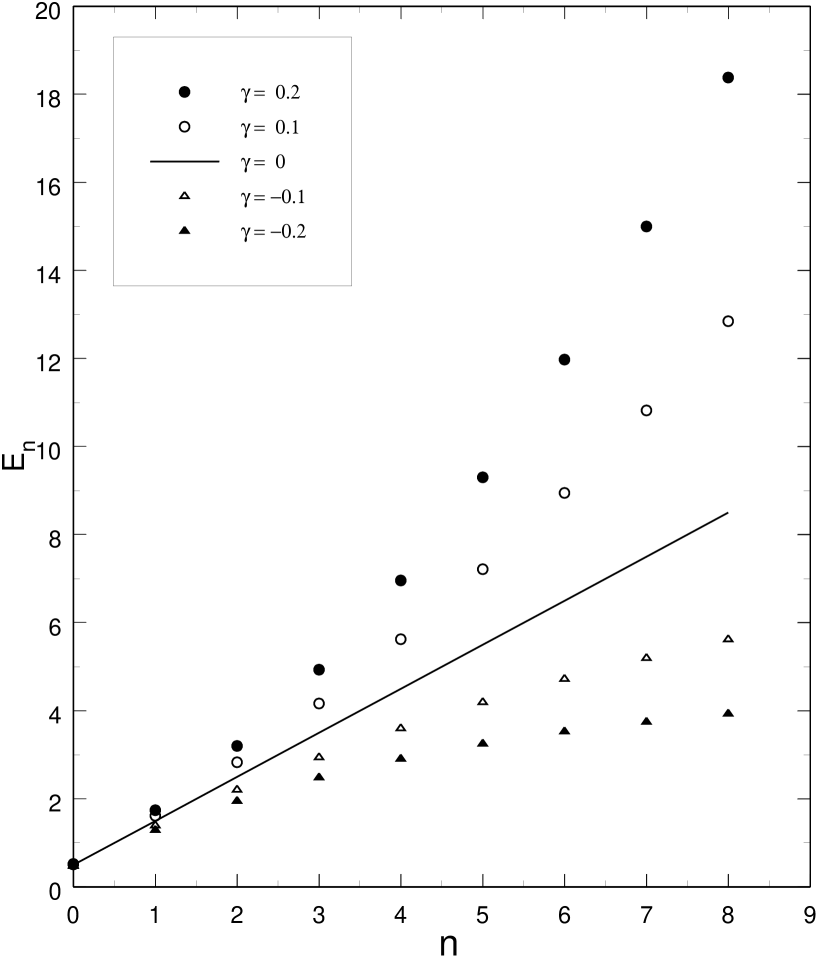
Figure 1: $E_{n}$ as function of n for the linear E-dependent harmonic oscillator, with $\gamma=0,\pm 0.1,\ {\rm and}\ \pm 0.2$. The solid line corresponds to $\gamma=0$, points above (below) correspond to $\gamma>0$ ($\gamma<0$).

In Fig. 1, the energy $E_{n}$ is presented as function of n for several values of $\gamma$ and $n\leq 8$. While positive values of $\gamma$ produce an increase of the level spacing as function of $n$, negative values of $\gamma$ compress the spectrum. For $\gamma<0$, $E_{n}$ is a monotonically increasing function of $n$. Asymptotically ($n\rightarrow\infty$), its derivative reaches $-\frac{24}{(2n+1)^{3}\gamma^{3}}$, and $E_{n}\approx-\frac{1}{\gamma}$. This limit ensures that $\lambda_{n}$ is real $\forall n$, with $\lambda_{n}\rightarrow 0$.

As stated in the preceding section, physically acceptable potentials must yield positive norms. In the present case, we have

$$C_{n}^{2}\int_{-\infty}^{\infty}e^{-\lambda_{n}x^{2}}h_{n}^{2}(\sqrt{\lambda_{n}}x)[1-\frac{\gamma}{2}\ x^{2}]dx=1\ ,$$ (23)

which gives

$$C_{n}^{2}\ =\ \frac{1}{2^{n}\ n!}\ \frac{\sqrt{\lambda_{n}}}{\sqrt{\pi}}\Big{[}1-\frac{\gamma}{4\lambda_{n}}(2n+1)\Big{]}^{-1}\ .$$ (24)

From Eqs. (16) and (21), we get

$$\frac{(2n+1)}{4}\gamma=\lambda_{n}-\sqrt{1+\frac{(2n+1)^{2}}{16}\gamma^{2}}\ .$$ (25)

Consequently, the norm is positive definite $\forall n$, irrespective of the sign of $\gamma$.

The modification of the scalar product affects also the calculation of expectation values. In the case of the mean square (ms) radius we obtain

$$\langle x^{2}\rangle_{n}=\frac{(2n+1)}{2\lambda_{n}}\Big{[}1-\frac{\gamma}{4\lambda_{n}}(2n+1)\Big{]}^{-1}\ \Big{[}1-\frac{3\gamma}{8\lambda_{n}}\frac{[(2n+1)^{2}+1]}{(2n+1)}\Big{]}\ .$$ (26)

For $\gamma$ positive, the sign of $\langle x^{2}\rangle_{n}$ is linked to the sign of the last term. It is easy to show that for $n\rightarrow\infty$ it takes the value 1/4, whereas for $n=0$, it becomes negative beyond $\gamma=\sqrt{16/3}$. Thus the question is, for which state the ms radius is positive definite. For $n=1$, it is straightforward to show (using Eqs. (16), (21)) that the last factor of Eq. (26) has no real root, and the ms radius is thus positive definite.

As the critical value $\gamma=\sqrt{16/3}$ is large compared to 1, one might expect to avoid contradictions for $\gamma<<1$. Unfortunately, explicit calculations of higher moments $\langle x^{k}\rangle_{n}$ ($k$ even) for few low $n$ states indicate that (up to the leading order):

$$\langle x^{k}\rangle_{n}\propto[1-\frac{\gamma\ (k+1)}{4\lambda_{n}}]\ .$$ (27)

Thus, for fixed $n$ and positive $\gamma$, there will always be a value of $k$, beyond which $\langle x^{k}\rangle_{n}$ becomes negative.

The above example clearly demonstrates that ad-hoc modification of the operation which should play the role of the scalar product and the positivity of the “norm” of the assumed energy eigenfunctions are not sufficient to ensure the positivity of the expectation value of a positive definite operator. It underlines an internal inconsistency for $\gamma>0$.

As far as the closure relation is concerned, as stated in the preceding section, the ansatz (9) seems to be valid for a linear energy dependence. It is straightforward to get a numerical test by calculating, for instance,

$$\langle x^{2}\rangle_{0}=\sum_{n}|\langle n|x|0\rangle|^{2}\ .$$ (28)

Up to linear terms in $\gamma$, we verified that

$$\langle x^{2}\rangle_{0}\approx\frac{1}{2}(1-\frac{3}{4}\gamma)\approx|\langle 1|x|0\rangle|^{2}\ .$$ (29)

Higher contributions, $|\langle n|x|0\rangle|^{2}\ ,\ \ {\rm where}\ \ n\geq 3$, are proportional at least to $\gamma^{2}$. This results from the fact that in the ordinary harmonic oscillator ($\gamma=0$), the $x$ operator connects only states which differ by one quantum of energy. It is obviously a tedious work to check Eq. (28) to all orders in $\gamma$. However, since we know the exact value of $\langle x^{2}\rangle_{0}$, we can estimate the contributions from the first excited states and discuss the convergence of the series expansion. As an example, we have calculated the first two terms for $0.01\leq|\gamma|\leq 0.50$. The results are displayed in Table 1. They are compared with the exact values and with the estimates obtained keeping only contributions linear in $\gamma$. Whereas the latter approximation becomes inaccurate by few percent beyond $\gamma=0.25$, the convergence seems rapid. The contribution of the third excited state is less than 2 % for $\gamma=0.5$.

As the second example, we have tested the same way

$$\langle x^{4}\rangle_{0}=\sum_{n}|<0|x^{2}|n>|^{2}\approx|\langle 0|x^{2}|0\rangle|^{2}+|\langle 2|x^{2}|0\rangle|^{2}\approx\frac{3}{4}(1-\frac{3}{2}\gamma)\ ,$$ (30)

keeping only terms linear in $\gamma$. In Table 2, we compare the exact values with the linear estimates and with the sums of the series expansion as a function of $n_{max}$ (the highest state involved in the sum). The situation is somewhat worse than for $<x^{2}>_{0}$ : the linear approximation is less efficient and the convergence of the series expansion is slower.

The above results support the extension (9) of the closure relation. They also underline the care one has to take when using $\gamma$ as a small parameter in a series expansion. On the other hand, for $\gamma>0$, we note a tendency to overpass the exact value, which appears beyond $\gamma=0.4$ for $<x^{2}>_{0}$ and beyond $\gamma=0.35$ for $<x^{4}>_{0}$. We have verified that this effect is not due to numerical uncertainties. Again, it is a signature of the deficiency of the algorithm for $\gamma>0$.

The consequence of the modification of commutation relations can be illustrated on the dipole sum rule. We recall that it is obtained by averaging over the ground state the double commutator $\Big{[}[H,x],x\Big{]}$.

According to Eq. (13), we have

$$\Big{[}[H,x],x\Big{]}=-\frac{1}{1-\gamma x^{2}/2}\ .$$ (31)

and the ground state expectation value yields

$$\sum_{n}(E_{n}-E_{0})|\langle n|x|0\rangle|^{2}=\frac{1}{2}\langle 0|\Big{[}[H,x],x\Big{]}|0\rangle=\frac{1}{2}[1-\frac{\gamma}{4\lambda_{0}}]^{-1}\ .$$ (32)

As a numerical test, we adopted several maximum values $n_{max}$ of $n$ considered in the sum. Results are displayed in Table 3 for $n_{max}=1$ up to 7. They are compared with the exact value given by the last term of Eq. (32). The convergence rate is slower as $\gamma$ increases, as expected. The convergence towards the right result for the low $\gamma$ values supports the validity of the rules used to derive Eq. (32). For $\gamma>0$, contrary to the $<x^{2}>_{0}$ and $<x^{4}>_{0}$ cases, the sum seems to converge toward the exact value. This comes from the fact that the leading contribution to the ground state average of Eq. (32) is the norm, for which the orthonormality of the wave functions ensures that $\sum_{n}|<n|0>|^{2}=1$.

2.2.2 $\sqrt{E}$ - dependence

The $\sqrt{E_{n}}$ case is chosen for the sake of comparison with the results of the previous example. A smoother energy dependence should generate weaker effects. On the other hand, the simpler generalization (9) of the closure relation is valid only approximately. Therefore, we do not expect to calculate expectation values of commutators (13,14) with unlimited accuracy.

The eigenvalues of Eq. (15) are in this case given by

$$4E_{n}^{2}-(2n+1)^{2}[1+\gamma\sqrt{E_{n}}]=0\ .$$ (33)

On the real half-plane $E_{n}\geq 0$, for each sign of $\gamma$ and each $n$, there exists a single real eigenvalue leading to square integrable wave function. The spectrum exhibits the same features as the linear $E_{n}$-dependence.

For small positive $\gamma$ (typically $\gamma\leq 0.2$) and few lowest states ($n\leq 3$), a perturbative estimate yields

$$E_{n}\approx(n+\frac{1}{2})[1+\frac{\gamma}{2}\sqrt{\frac{(2n+1)}{2}}]\ .$$ (34)

For $\gamma<0$, the large $n$ limit is given by

$$\lim_{n\to\infty}E_{n}=\frac{1}{\gamma^{2}}\ .$$ (35)

As in the linear $E_{n}$-dependence, it ensures $\lambda_{n}$ to be real and reaching 0 as $n\rightarrow\infty$.

The norms and the (assumed) predictions of the average values of observables are calculated by introducing the multiplicative factor

$$1-\frac{\gamma}{2(\sqrt{E_{n}}+\sqrt{E_{n^{\prime}}})}x^{2}\ .$$ (36)

The norms, given by

$$C_{n}^{2}=\frac{1}{2^{n}n!}\frac{\sqrt{\lambda_{n}}}{\sqrt{\pi}}\Big{[}1-\frac{1}{8\lambda_{n}}\gamma\frac{(2n+1)}{\sqrt{E_{n}}}\Big{]}^{-1},$$ (37)

are positive definite as can be proved using Eq. (21) and (33).

The ms radius

$$\langle x^{2}\rangle_{n}=\frac{2n+1}{2\lambda_{n}}\Big{[}1-\frac{1}{8\sqrt{E_{n}}}\frac{\gamma(2n+1)}{\lambda_{n}}\Big{]}^{-1}\Big{[}1-\frac{3}{16\sqrt{E_{n}}}\ \frac{\gamma[(2n+1)^{2}+1]}{\lambda_{n}(2n+1)}\Big{]}\$$ (38)

is positive definite $\forall n$, as well. On the other hand, for $\langle x^{k}\rangle_{n}$, the same reasoning as for the linear case yields (up to the leading order)

$$\langle x^{k}\rangle_{n}\propto[1-\frac{\gamma(K+1)}{4\lambda_{n}\sqrt{E_{n}}}]\ .$$ (39)

For fixed $\gamma>0$ and $n$, there exists a value of $k$ beyond which $\langle x^{k}\rangle_{n}$ becomes negative. In spite of a smoother energy dependence than in the linear case, very similar problems occur in the case of expectation values of positive definite operators for $\gamma>0$.

Because $\varphi_{nn^{\prime}}$ are energy dependent, the ”closure ansatz” has no chance to be given by the simple extension (9). Nevertheless, one can estimate the correction terms. To fix the order of magnitude, we take Eq. (10) for $\Psi_{j}=\Psi_{0}$, where

$$[\varphi_{nn}(x)-\varphi_{n0}(x)]=\frac{\gamma\ x^{2}}{2}\ [\ \frac{1}{2\sqrt{E_{n}}}-\frac{1}{(\sqrt{E_{0}}+\sqrt{E_{n}})}\ ]\ .$$ (40)

We consider the first two contributions to the sum of Eq (10). Because of parity, they arise from $\Psi_{2}$ and $\Psi_{4}$. The results are displayed in Table 4. The correction is small in the range of considered $\gamma$ values, but not necessary negligible. It is expected to decrease with increasing $n$.

Neglecting the correction terms, we can perform the same tests as in the preceding subsection. Up to linear terms in $\gamma$,

$$\langle x^{2}\rangle_{0}\approx\frac{1}{2}(1-\frac{\gamma}{\sqrt{2}})\ \ {\rm is\ to\ be\ compared\ to}\ \ |\langle 1|x|0\rangle|^{2}\approx\frac{1}{2}(1-0.65\gamma)\ .$$

The difference between the two estimates is of the same order as the correction terms listed in Table 4.

A more quantitative estimate is displayed in Table 5. The exact value of $\langle x^{2}\rangle_{0}$ is compared with the sums $\sum_{n}^{n_{max}}|\langle n|x|0\rangle|^{2}$, with $n_{max}$ = 1,2 and 3. The series expansion converges rather rapidly but not to the exact value. The discrepancies are of the same order as the one observed in the above expression limited to terms linear in $\gamma$.

2.2.3 Further energy dependences

The above two examples yield an overview of the difficulties linked to the energy dependence of the potential in a wave equation. There is no need to pursue this investigation much further. One point, however, is worth mentioning. It concerns the cases when higher powers of the energy dependence are considered. Take for instance $f(E_{n})=E_{n}^{2}$. It is easy to verify that the positive eigenvalues are given by

$$E_{n}=\frac{2n+1}{\sqrt{4-(2n+1)^{2}\gamma}}\ .$$ (41)

We note that for positive $\gamma$ there will always be a critical $n$ beyond which the eigenvalue becomes complex.

3 A quantum theory.

A toy model is well suited for illustrative purposes. However, in order to go beyond and check if it corresponds to a well defined theory, a more fundamental analysis is required. Mathematical aspects of theories with energy dependent potentials have been studied in ref. [12,13,5]. In particular, these works are devoted to the positivity of the norm and the occurance of pathologies [1].

Let us define (for a given Hilbert space $\mathcal{H}$) a Hamiltonian

$$\hat{H}(z)=\hat{H}_{0}+\hat{V}(z)\ ,$$ (42)

where $\hat{H}_{0}$ is a selfadjoint operator and there exists such a set $\mathcal{M}\subset\mathcal{R}$ that for any fixed value $z\in\mathcal{M}$ each of the operators $\hat{V}(z)$, $\hat{H}(z)$ is selfadjoint too.

Let us make attempt to construct a quantum theory (QT) in such a way that

1) the vectors $|\Psi>\in\mathcal{H}$, at least some of them, correspond to states of a physical system (here and in the following “state” is used in the sense of “pure state” only),

2) the time evolution of these states is determined by the equation

$$i\frac{d}{dt}|\Psi(t)>=\hat{H}(i\frac{d}{dt})|\Psi(t)>\ .$$ (43)

First of all, one should keep in mind the following requirements, which have to be satisfied by any QT :

i) Each state of the considered physical system is mapped to a ray in the corresponding Hilbert space (${\mathcal{H}}_{p}$).
ii) Each state of the considered system represents a linear combination of its stationary states.
iii) The initial state of the system (its state at $t_{0}$) uniquely determines its states at each later moment $t>t_{0}$ (provided the system was not submitted to any measurement and/or observation during the interval ($t_{0}$,$t>$ ).

The last requirement apparently limits the acceptable $z$-dependence of $\hat{V}(z)$ to the linear one only. But one can try to avoid this sharp restriction in the following way : the Hilbert space ${\mathcal{H}}_{p}$ need not be identical with $\mathcal{H}$. In fact, the two spaces might differ in 2 aspects :

a) some of the vectors from $\mathcal{H}$ need not belong to ${\mathcal{H}}_{p}$; these elements of $\mathcal{H}$ would not describe any state of the considered system, i.e., the vector space ${\mathcal{H}}_{p}$ could be a (proper) subspace of the vector space $\mathcal{H}$.

b) The vector space ${\mathcal{H}}_{p}$ could be endowed with a different scalar product ($\big{(}\cdot\ |\ \cdot>$ ) than the vector space $\mathcal{H}$. (We reserve the symbol $<\cdot|\cdot>$ for the scalar product in the Hilbert space $\mathcal{H}$). In other words, the Hilbert space ${\mathcal{H}}_{p}$ need not be a subspace of the Hilbert space $\mathcal{H}$.

From the requirement i) directly follows that a vector

$$|\Psi>\in{\mathcal{H}}_{p}\ \ ,\ \ |\Psi>\not=0$$ (44)

corresponds to a stationary state of the considered system if and only if there is such a real number $E$ that the vector valued function (of time)

$$|\Psi(t)>=e^{-iEt}|\Psi>$$ (45)

satisfies Eq. (43). Moreover, it is evident that the function (45) solves Eq. (43) if and only if the vector (44) satisfies the relation

$$(\hat{H}_{0}+\hat{V}(E)\ )\ |\Psi>=E\ |\Psi>\ \ .$$ (46)

It is customary to call this relation the (time independent) “Schrödinger equation with an energy dependent potential”.

Let us recall that $\forall E\in\mathcal{M}$ there $\exists\ |\Psi>\in\mathcal{H}$;

$$(\hat{H}_{0}+\hat{V}(E)\ )\ |\Psi>\ \in\ \mathcal{H}\ .$$ (47)

On the other hand (usually) for most of values $E\in\mathcal{M}$ none of

$$|\Psi>\ \in{\mathcal{H}}\ ,\ |\Psi>\not=0$$ (48)

satisfies the condition (46). To find out those values of $E$ for which Eq. (46) has nontrivial solution in $\mathcal{H}$, let us first of all consider the equation

$$\hat{H}(z)|\Psi>=E(z)\ |\Psi>\ .$$ (49)

For simplicity, we will limit our discussion to the case where $\forall z\in\mathcal{M}$ the spectrum of $\hat{H}(z)$ is purely discrete and non-degenerate. This means that for any fixed value $z\in\mathcal{M}$, to each eigenvalue $E_{n}(z)$ of $\hat{H}(z)$, there $\exists\ |\Psi(z)>\ \in\mathcal{H}$ :

$$\hat{H}(z)|\Psi_{n}(z)>=E_{n}(z)\ |\Psi_{n}(z)>\ ,\ \ \ |\Psi_{n}(z)>\not=0$$ (50)

and no other linearly independent solution of Eq. (46) with $E=E_{n}(z)$ exists in $\mathcal{H}$. It may happen that for a given value of $n$ there exist such values $z\in\mathcal{M}$ that the relation

$$E_{n}(z)=z$$ (51)

holds. In the following, we will enumerate by the index $n$ only those eigenvalues of $\hat{H}(z)$ for which Eq. (51) has at least one solution in $\mathcal{M}$. Those values of $z\in\mathcal{M}$ which satisfy the relation (51) will be denoted as

$$z_{m}^{(n)}\ ,\ m=1,\ldots,M_{n}\geq 1\ ,$$ (52)

i.e., $z_{m}^{(n)}$ are those elements of $\mathcal{M}$ for which

$$E_{n}(z_{m}^{(n)})=z_{m}^{(n)}\ .$$ (53)

Due to Eq. (50) we have

$$\hat{H}(z_{m}^{(n)})\ |\Psi_{n}(z_{m}^{(n)})>=E_{n}(z_{m}^{(n)})\ |\Psi_{n}(z_{m}^{(n)})>=z_{m}^{(n)}\ |\Psi_{n}(z_{m}^{(n)})>\ .$$ (54)

Moreover, due to the assumed non-degeneracy of the $\hat{H}(z)$ spectrum, we know that for each given $z_{m}^{(n)}$ the last equation has one and only one linearly independent solution in $\mathcal{H}$. Let us denote it as $|\Psi_{m}^{(n)}>$. Without any loss of generality, on can impose the normalization condition

$$<\Psi_{m}^{(n)}\ |\ \Psi_{m}^{(n)}>=1\ .$$ (55)

In order to simplify symbolics, let us switch from the two-index to one-index notation

$$\{(n),m\}\rightarrow j\equiv\sum_{k=0}^{n-1}M_{k}+m\ ,\ \ {\rm where}\ \ M_{0}=0$$ (56)

and

$$z_{j}\equiv z_{m}^{(n)}\ ,\ |\Psi_{j}>\equiv\ |\Psi_{m}^{(n)}>\ .$$ (57)

If one accepts the “philosophy of energy dependent potential”, then each of the values

$$z_{j}\ ,\ j=1,\ldots,N\equiv\sum_{k}M_{k}$$ (58)

represents an energy level of the considered system (and each energy level coincides with one of the values (58)) and the vector $|\Psi_{j}>$ unambiguously describes the corresponding stationary state.

In order to satisfy the aforementioned condition ii), one has to require $\forall|\Psi>\in{\mathcal{H}}_{p}$ to be expressible in the form

$$|\Psi>=\sum_{j}\ c_{j}\ |\Psi_{j}>\ ,\ \ {\rm where}\ \ c_{j}=const.\ .$$ (59)

Such a vector space ${\mathcal{H}}_{p}$ could represent Hilbert space assigned to a physical system in the framework of any QT only if it could be endowed with such a scalar product $\big{(}\cdot|\cdot>$ that the orthogonality condition

$$\big{(}\Psi_{j}|\Psi_{k}>=0\ \ ,\ \ \forall j\not=k\$$ (60)

would be guaranteed. On the other hand,

$$(\hat{H}_{0}+\hat{V}(z_{j})\ |\ \Psi_{j}>=z_{j}\ |\Psi_{j}>$$ (61)

implies (due to selfadjointness of $\hat{H}_{0}$ and $\hat{V}(z)$) that the identity

$$(z_{j}-z_{k})<\Psi_{k}|\Psi_{j}>=<\Psi_{k}|[\hat{V}(z_{j})-\hat{V}(z_{k})]|\Psi_{j}>\$$ (62)

is valid $\forall j\not=k$.

Hence, the requirement (60) would be automatically satisfied if the scalar product in ${\mathcal{H}}_{p}$ is defined in such a way that

$$\big{(}\Psi_{j}|\Psi_{k}>\equiv<\Psi_{j}|\hat{W}_{jk}|\Psi_{k}>\ ,$$ (63)

where

$$\hat{W}_{jk}\equiv 1-\hat{Q}_{jk}$$ (64)

and

$$\hat{Q}_{jk}\equiv\frac{\hat{V}(z_{j})-\hat{V}(z_{k})}{z_{j}-z_{k}}\ \ ,\ \ \forall\ j\not=k\ \ .$$ (65)

In order to define the scalar product in ${\mathcal{H}}_{p}$, it remains to specify the meaning of the r.h.s. of the expression (65) for $j=k$. It is tempting to take

$$\hat{Q}_{jj}\equiv\frac{d\hat{V}}{dz}(z_{j})\ .$$ (66)

We are not going to dwell on arguments neither in favor nor against this specific choice of the “scalar product” $\big{(}\cdot|\cdot>$, utilized e.g. in Eq. (8). Let us stress instead that one can face serious problems when introducing any scalar product $\big{(}\cdot|\cdot>$, which would guarantee fulfillment of the requirement (60). The point is that the conditions (54) and (55) define the set of vectors

$$|\Psi_{j}>\ ,\ j=1,\ldots,N$$ (67)

(up to phase factors) uniquely but they do not imply the linear independence of all the vectors (68). One should not forget that the requirements (54) and (55) do not guarantee that all the vectors (67) are eigenvectors of a common selfadjoint operator. On the other hand, if

$$|\Psi_{j}>=\sum_{k\not=j}C_{k}\ |\Psi_{k}>\ ,$$ (68)

then from the condition (60) follows

$$\big{(}\Psi_{j}|\Psi_{j}>=0\ ,$$ (69)

i.e., $|\Psi_{j}>$ would be the null vector. But from the condition (55) we know that it is not so. This means that if not all the vectors (68) are linearly independent, than it is impossible to define any scalar product $\big{(}\cdot|\cdot>$ in ${\mathcal{H}}_{p}$ in such a way that the condition (60) is satisfied. Especially, this means that in such a case
i) the relations (63)-(66) do not define a scalar product
ii) it is impossible to modify the r.h.s. of equation (66) in such a way that the relations (63)-(66) would define a scalar product in ${\mathcal{H}}_{p}$.
In other words, in such a case, the aforementioned algorithm does not represent any QT.

On the other hand, it is clear that for any given quantities $\hat{H}_{0}$, $\hat{V}(z)$ there exists (at least one) such a set $\mathcal{M}$ that all the vectors (67) are linearly independent. Therefore, at least in principle, one can avoid the above indicated problem simply by a “proper choice” of the set $\mathcal{M}$.

Of course one should keep in mind that
$\alpha$) the requirement of the linear independence of the vectors (67) does not determine the set $\mathcal{M}$ uniquely. ( It could be tempting to choose $\mathcal{M}$ as the largest subset of real values $z$ for which the operators $\hat{H}(z)$, $\hat{V}(z)$ are selfadjoint and all the vectors (67) are linearly independent. But generally there still could be more then one subset of $\mathcal{R}$ which fulfills all these conditions.)
$\beta$) the “energy spectrum” produced by such an algorithm substantially depends on the     particular choice of the set $\mathcal{M}$.

The main moral from these observations is that the specification of the operator (valued function) (42) itself need not determine uniquely the energy spectrum of the corresponding physical system with energy dependent potential.

To proceed further in our analysis, let us from now on assume that the set $\mathcal{M}$ is already chosen in such a way that all the vectors (67) are linearly independent, and therefore the vector space ${\mathcal{H}}_{p}$ (59) is a $N$-dimensional subspace of the vector space $\mathcal{H}$. Let us also define vectors

$$|\Psi^{j}>\equiv A^{(j)}\ |\Psi_{j}>\ ,$$ (70)

where $A^{(j)}$ are non-vanishing constants determined (up to their phase factors) by the requirement

$$\big{(}\Psi^{j}|\Psi^{k}>=\delta_{jk}\ ;\ j,k=1,\ldots,N\ ,$$ (71)

once the scalar product $\big{(}\cdot|\cdot>$ in ${\mathcal{H}}_{p}$ is specified.

Since ${\mathcal{H}}_{p}$ is an $N$-dimensional subspace of $\mathcal{H}$, there exist such vectors

$$|\chi_{j}>\ \in{\mathcal{H}}_{p}\ ,\ j=1,\ldots,N$$ (72)

that

$$<\chi_{j}|\chi_{k}>=\delta_{jk}\ ,\ j,k=1,\ldots,N\ ,$$ (73)

and any vector $|\Psi>\ \in{\mathcal{H}}_{p}$ can be expressed as a linear combination of them. Especially each vector (70) is expressible as

$$|\Psi^{j}>=\sum_{k=1}^{N}\xi_{kj}\ |\chi_{k}>\ ,\ j=1,\ldots,N$$ (74)

and the constants

$$\xi_{kj}=<\chi_{k}|\Psi^{j}>\ .$$ (75)

Evidently these relations could be expressed also in the form

$$|\Psi^{j}>=\hat{\xi}|\chi_{j}>\ ,\ j=1,\ldots,N\ ,$$ (76)

where

$$\hat{\xi}=\sum_{k=1}^{N}|\Psi^{k}><\chi_{k}|=\sum_{\ell,k=1}^{N}\xi_{\ell k}|\chi_{\ell}><\chi_{k}|$$ (77)

is a linear operator (on ${\mathcal{H}}_{p}$) and

$$\xi_{kj}=<\chi_{k}|\hat{\xi}|\chi_{j}>\ .$$ (78)

Moreover, due to the linear independence of all $N$ vectors (70), the relations (76) have to be invertible, i.e., the operator $\hat{\xi}$ is nonsingular. Therefore the relations (76) are equivalently expressed as

$$|\chi_{j}>=\hat{\eta}|\Psi^{j}>\ ,\ j=1,\ldots,N\ ,$$ (79)

where the linear operator (on ${\mathcal{H}}_{p}$)

$$\hat{\eta}\equiv\hat{\xi}^{-1}\ .$$ (80)

Let us define $\forall\ |\Psi>\ \in\ {\mathcal{H}}_{p}$ the corresponding vector (in ${\mathcal{H}}_{p}$)

$$|\tilde{\Psi}>\equiv\hat{\eta}|\Psi>\ .$$ (81)

Recalling Eq. (79) one can see that

$$|\tilde{\Psi}^{j}>=|\chi_{j}>$$ (82)

and hence the equivalence

$$|\Psi>=\sum_{j=1}^{N}c_{j}|\Psi^{j}>\ \Leftrightarrow|\tilde{\Psi}>=\sum_{j=1}^{N}c_{j}|\chi_{j}>$$ (83)

holds. Therefore, for any vector $|\Psi>,|\Phi>\ \in{\mathcal{H}}_{p}$ the relation

$$\big{(}\Phi|\Psi>=<\tilde{\Phi}|\tilde{\Psi}>$$ (84)

holds. It means that the scalar product $\big{(}\cdot|\cdot>$ could be expressed in terms of the scalar product $<\cdot|\cdot>$ as

$$\big{(}\Phi|\Psi>=<\Phi|\hat{\kappa}|\Psi>\ ,$$ (85)

where the linear operator

$$\hat{\kappa}\equiv\hat{\eta}^{+}\hat{\eta}\ .$$ (86)

It is useful to express Eq. (85) as a relation between two different bra-vectors related to the same ket by the two different definitions of the scalar product (on the same vector space ${\mathcal{H}}_{p}$) :

$$\big{(}\Phi|=<\Phi|\hat{\kappa}\ .$$ (87)

One should not overlook that using this formalism one can e.g. express the closure relation corresponding to the orthonormality condition (71) in the following simple form

$$\sum_{j=1}^{N}|\Psi^{j}>\big{(}\Psi^{j}|=1\ .\ \ \ \ \ \ \ \ \ \ \ \ \ {\rm 87a)}$$

Needless to say that this relation is equivalent to the closure

$$\sum_{j=1}^{N}|\chi_{j}><\chi_{j}|=1\ .$$

In order that the considered algorithm could provide a QT of a physical system, one has to assign to each observable $A$ the corresponding selfadjoint operator $\hat{A}$. At this point, it is important to keep in mind that the notion of conjugation of linear operators depends on the choice of the scalar product. We have tacitly used the symbol $\hat{A}^{+}$ to denote the operator conjugated to the operator $\hat{A}$ in the sense of the scalar product $<\cdot|\cdot>$, i.e., the relation

$$<\Psi|\hat{A}^{+}|\Phi>=<\Phi|\hat{A}|\Psi>^{*}\$$ (88)

holds.

Let us introduce the symbol $\hat{A}^{\#}$ to denote the operator conjugated to $\hat{A}$ in the sense of the scalar product $\big{(}\cdot|\cdot>$, i.e.. the relation

$$\big{(}\Psi|\hat{A}^{\#}|\Phi>=\big{(}\Phi|\hat{A}|\Psi>^{*}$$ (89)

holds. By using the relation (87) one finds

$$\big{(}\Phi|\hat{A}|\Psi>^{*}=<\Phi|\hat{\kappa}\hat{A}|\Psi>^{*}=<\Psi|\hat{A}^{+}\hat{\kappa}|\Phi>=\big{(}\Psi|\hat{\kappa}^{-1}\ \hat{A}^{+}\ \hat{\kappa}|\Phi>$$ (90)

and therefore

$$\hat{A}^{\#}=\hat{\kappa}^{-1}\ \hat{A}^{+}\ \hat{\kappa}=\hat{\xi}\hat{\xi}^{+}\ \hat{A}^{+}\ \hat{\eta}^{+}\hat{\eta}\ .$$ (91)

One can utilize the formal relations

$$\big{(}|\Psi>\big{)}^{+}=<\Psi|\ \ ;\ \big{(}|\Psi>\big{)}^{\#}=\big{(}\Psi|\ ,$$ (92)

and therefore

$$\big{(}|\Psi><\phi|\big{)}^{+}=|\phi><\Psi|\ \ ;\ \big{(}|\Psi>\big{(}\phi|\big{)}^{\#}=|\phi>\big{(}\Psi|\ ,$$ (93)

etc. It is also useful to notice that the operator (86) is selfadjoint from the point of view of both scalar products, i.e.

$$\hat{\kappa}=\hat{\kappa}^{+}=\hat{\kappa}^{\#}\ .$$ (94)

Needless to say that when we required (below Eq. (87)) the operator $\hat{A}$, assigned in the considered algorithm to an observable $A$, to be selfadjoint, we meant that the relation

$$\hat{A}^{\#}=\hat{A}$$ (95)

has to hold.

The discussed algorithm may appear as a sort of QT which is still “peculiar” in two aspects:
i) the (total) energy is the only observable to which no selfadjoint operator was assigned,
ii) evolution of the state has not been described by an “ordinary Schrödinger equation”.

Let us show now that both of these points could be circumvented, namely, that the considered algorithm may be equivalently expressed in the form of an ordinary quantum
mechanics:

Let us define the operator

$$\hat{H}\equiv\sum_{j=1}^{N}z_{j}|\Psi^{J}>\big{(}\Psi^{j}|\ .$$ (96)

From Eqs. (93), (54) and (70) follows that the relations

$$\hat{H}^{\#}=\hat{H}\ ,$$ (97)

$$\hat{H}|\Psi^{j}>=E_{j}|\Psi^{j}>\ ,\ {\rm where}\ E_{j}\equiv z_{j}\ ,$$ (98)

are guaranteed. Moreover, from Eqs. (45), (59) and (70) follows that the solution (43) with the initial condition

$$|\Psi(t_{0})>=|\Psi>\ \in\ {\mathcal{H}}_{p}$$ (99)

may be expressed in the form

$$|\Psi(t)>=\sum_{j}d_{j}e^{-iE_{j}t}|\Psi^{j}>\ ,\ {\rm where}\ d_{j}\equiv\frac{c_{j}}{A^{(j)}}$$ (100)

and hence the “ordinary Schrödinger equation”

$$i\frac{d}{dt}|\Psi(t)>=\hat{H}|\Psi(t)>$$ (101)

holds.

Therefore the considered QT (with an “energy dependent potential”) could be equivalently rephrased as an “ordinary quantum mechanics” (QM1) in such a way that
1) the Hilbert space of the corresponding system is identified with the vector space ${\mathcal{H}}_{p}\ \subset\ \mathcal{H}$ endowed with the scalar product $\big{(}\cdot|\cdot>$,
2) the Hamiltonian is identified with the operator (96).

Actually, one can rephrase the considered QT also as an “ordinary quantum mechanics” (QM2) of the same physical system in such a way that the Hilbert space assigned to this system is identified with the subspace ${\mathcal{H}}_{p}\ \subset\ \mathcal{H}$, i.e. with the vector space ${\mathcal{H}}_{p}$ endowed with the scalar product $<\cdot|\cdot>$.

To this end, it is sufficient to realize that once one associates to each linear operator $\hat{A}$ the operator

$$\hat{\tilde{A}}=\hat{\eta}\hat{A}\hat{\xi}\ ,$$ (102)

then, from the definition (81), one immediately sees that $\forall|\Psi>\ \in\ {\mathcal{H}}_{p}$
the relation $|\Phi>=\hat{A}\ |\Psi>$ is equivalent to $|\tilde{\Phi}>=\hat{\tilde{A}}|\tilde{\Psi}>$,
and the relation $\hat{A}^{\#}=\hat{B}$ might be equivalently expressed as $\hat{\tilde{A}}^{+}=\hat{\tilde{B}}$.

On the other hand, from the formulae (96), (87) and (82), one immediately obtains

$$\hat{\tilde{H}}=\sum_{j=1}^{N}z_{j}\hat{\eta}|\Psi^{j}><\Psi^{j}|\hat{\eta}^{+}\hat{\eta}\hat{\xi}=\sum_{j=1}^{N}z_{j}|\chi_{j}><\chi_{j}|\ .$$ (103)

In this case, the stationary states are described by the vectors $|\chi_{j}>$ and the evolution of the states of the considered system is described by the Schrödinger equation

$$i\frac{d}{dt}|\tilde{\Psi}(t)>=\hat{\tilde{H}}|\tilde{\Psi}(t)>\ .$$ (104)

The operators associated to observables are now selfadjoint in the sense of the relation

$$\hat{\tilde{A}}^{+}=\hat{\tilde{A}}\ .$$ (105)

We have seen that the considered algorithm could represent a QT if and only if the operation $\big{(}\cdot|\cdot>$ (introduced as a part of this algorithm) is expressible in the form (85), where $\hat{\kappa}$ is a selfadjoint positive definite operator. How can one check whether this condition is met?
First, it would be useful to express the operator $\hat{\eta}$ in the form

$$\hat{\eta}\equiv\sum_{j,k=1}^{N}\eta_{jk}|\chi_{j}><\chi_{k}|\ .$$ (106)

One finds that

$$\eta_{jk}=<\chi_{j}|\hat{\eta}|\chi_{k}>=<\Psi^{j}|\hat{\eta}^{+}\hat{\eta}|\chi_{k}>=\big{(}\Psi^{j}|\chi_{k}>\ .$$ (107)

This means that the coefficients on the r.h.s of Eq. (106) are identical with the coefficients in the expression

$$|\chi_{j}>=\sum_{k=1}^{N}\eta_{kj}|\Psi^{k}>\ .$$ (108)

Therefore one can obtain the operator corresponding to any (arbitrarily chosen) orthonormal basis (in the sense of relation (73))

$$\big{\{}\ |\chi_{j}>,\ j=1,\ldots,N\big{\}}$$ (109)

where each of its elements is expressed as a linear combination (108) with the coefficients $\eta_{kj}$ utilized in Eq. (106).

Once the operator $\hat{\eta}$ is known, one can check whether all the eigenvalues of the operator (94)

$$\hat{\kappa}\equiv\hat{\eta}^{+}\hat{\eta}$$ (110)

are non-vanishing. (Needless to say that the operator $\hat{\kappa}$ is uniquely determined by the operation $\big{(}\cdot|\cdot>$. The freedom in the choice of the operator $\hat{\eta}$ is just a trivial consequence of the fact that predictions of any (ordinary) quantum theory are invariant under arbitrary unitary transformations.) If it is the case then the considered algorithm could represent a QT. In the following we shall already tacitly assume that the operation $\big{(}\cdot|\cdot>$ is introduced in the considered algorithm in such a way that it can be interpreted as a scalar product in ${\mathcal{H}}_{p}$.

We have seen that this QT might be equivalently rephrased as a QM1 as well as a QM2. For passing from the QT to the QM2, the knowledge of the operator $\hat{\eta}$ appears essential (see Eqs. (102), (103) and (81)). We have already discussed the steps which could in principle lead to the construction of $\hat{\eta}$. Unfortunately, to proceed this way in practice usually represents a formidably complicated task. One naturally asks whether there exist any simpler way leading to the same goal.

In fact, it is easy to find a more straightforward procedure, at least for one particular case. Let

$$\hat{V}(z)=z\hat{V}$$ (111)

and the operator $\big{(}\cdot|\cdot>$ is defined by the formulae (63)-(66). In the case (111), the formula (64) simplifies to

$$\hat{W}_{jk}=1-\hat{V}\ ,$$ (112)

and therefore (cf. Eqs. (63) and (85))

$$\hat{\kappa}=1-\hat{V}\ .$$ (113)

Such an algorithm might represent a QT only if all values from the spectrum of the operator $\hat{V}$ are smaller than 1. The evolution equation (43) can be rewritten as

$$i\frac{d}{dt}(1-\hat{V})|\Psi(t)>=\hat{H}_{0}|\Psi(t)>$$ (114)

or equivalently as

$$i\frac{d}{dt}|\tilde{\Psi}(t)>=\hat{\xi}\hat{H}_{0}\hat{\xi}|\tilde{\Psi}(t)>\ ,$$ (115)

where we have used the notation (81):

$$|\tilde{\Psi}(t)>\equiv\hat{\eta}|\Psi(t)>\ ,$$ (116)

and without any loss of generality we have identified

$$\hat{\eta}=\hat{\eta}^{+}\equiv\sqrt{\hat{\kappa}}=\sqrt{1-\hat{V}}\ .$$ (117)

The equation (115) is of course nothing else than the (ordinary) Schrödinger eq. (104) with the Hamiltonian

$$\hat{\tilde{H}}=\hat{\xi}\hat{H}_{0}\hat{\xi}\ ,$$ (118)

where

$$\hat{\xi}=[1-\hat{V}]^{-1/2}\ .$$ (119)

Therefore, in this case we have reached the QM2, which is equivalent to the QT, just for free. Let us recall that in the framework of QM2, to each observable $A$ is assigned an operator $\hat{\tilde{A}}$, which fulfills the condition (105). In particular (in the considered case), the operator assigned to the (total) energy is given by formula (118).

From Eq.(102) follows that the operator $\hat{A}$, which is in the framework of QM1 associated to the observable $A$, is related to the operator $\hat{\tilde{A}}$ associated to the same observable in the framework of QM2 as follows

$$\hat{A}=\hat{\xi}\hat{\tilde{A}}\hat{\eta}\ ,$$

i.e.

$$\hat{A}=\frac{1}{\sqrt{(1-\hat{V})}}\hat{\tilde{A}}\sqrt{(1-\hat{V})}\ .$$ (120)

Especially, the Hamiltonian in the QM1 is the operator

$$\hat{H}=\hat{\xi}\hat{\tilde{H}}\hat{\eta}=\hat{\xi}^{2}\hat{H}_{0}\ ,$$ (121)

i.e.

$$\hat{H}=\frac{1}{1-\hat{V}}\hat{H}_{0}\ .$$ (122)

4 The toy model revisited.

In the light of the preceding section, we are going to re-examine our toy model. We will present an example of QT which reduces to QM1 or QM2. Let us consider the special case when

$${\mathcal{H}}\equiv L^{2}(-\infty,\infty)\ ,$$ (123)

$$\hat{H}_{0}\equiv-\frac{1}{2}\frac{d^{2}}{dx^{2}}+V_{0}(x)\ ,$$ (124)

$$\hat{V}=V(x)\ ,$$ (125)

and the real function $V$ fulfills the condition

$$V(x)<1\ \ \forall x\ \in\ (-\infty,\infty)\ .$$

Physically, this should be a one dimensional version of QT of a particle in an external field.

In this case

$$\hat{\tilde{H}}=\frac{1}{1-V}\Big{\{}V_{0}-\frac{1}{2}\Big{[}\frac{d^{2}}{dx^{2}}+\frac{V^{\prime}}{1-V}\ \frac{d}{dx}+\frac{1}{4}\ \frac{2V^{\prime\prime}(1-V)+3V^{\prime 2}}{(1-V)^{2}}\Big{]}\Big{\}}\ .$$ (126)

To be more specific, let us take

$$V(x)=-Kx^{2}\ ,\ K>0\ .$$ (127)

Then

$$\hat{\tilde{H}}=\frac{1}{1+Kx^{2}}\Big{\{}V_{0}(x)-\frac{1}{2}\Big{[}\frac{d^{2}}{dx^{2}}-\frac{2Kx}{1+Kx^{2}}\ \frac{d}{dx}-K\ \frac{1-2Kx^{2}}{(1+Kx^{2})^{2}}\Big{]}\Big{\}}\ .$$ (128)

To obtain the energy spectrum, one has to find those values of the parameter $E$ for which the differential equation

$$\Big{\{}-\frac{1}{2}\Big{[}\frac{d^{2}}{dx^{2}}-\frac{2Kx}{1+Kx^{2}}\ \frac{d}{dx}-K\ \frac{1-2Kx^{2}}{(1+Kx^{2})^{2}}\Big{]}+V_{0}(x)\Big{\}}\chi_{E}(x)=E(1+Kx^{2})\chi_{E}(x)$$ (129)

has solutions in ${\mathcal{H}}_{p}$ of QM2, i.e., which satisfy the integrability condition

$$\int_{-\infty}^{\infty}|\chi_{E}(x)|^{2}dx<\infty\ .$$ (130)

(For simplicity sake, we are explicitly describing here the procedure which concerns only the discrete part of the energy spectrum).

To be even more specific, let us consider the special case when

$$V_{0}(x)=Ax^{2}\ ,\ A>0\ .$$ (131)

Then Eq. (129) yields

$$\frac{1}{2}\chi^{\prime\prime}+\frac{Kx}{(1+Kx^{2})}\chi^{\prime}-\Big{[}\frac{K}{2}\ \frac{1-2Kx^{2}}{(1+Kx^{2})^{2}}+E+(EK-A)x^{2}\Big{]}\chi=0\ .$$ (132)

In the asymptotic region $|x|\rightarrow\infty$, Eq. (137) acquires the form

$$\chi^{\prime\prime}+\lambda^{2}x^{2}\chi\simeq 0\ ,$$ (133)

where

$$\lambda^{2}(E)=2(A-KE)\ .$$ (134)

Thus, for each real value of the parameter E, one can choose 2 independent solutions of Eq. (132) in such a way that their behavior in the asymptotic region $x\rightarrow\infty$ is dominated by the factor

$$e^{-\frac{\lambda(E)}{2}x^{2}}\ \ {\rm and}\ \ e^{\frac{\lambda(E)}{2}x^{2}}\ ,$$ (135)

respectively. Similarly, one can choose 2 independent solutions of (132) in such a way that their behavior in the asymptotic region $x\rightarrow-\infty$ is also dominated by the factor (135).

For $E>\frac{A}{K}$, $\lambda(E)$ is purely imaginary, and consequently both independent solutions oscillate in both asymptotic regions. This is why we strongly suspect that each value $E\ \in(\frac{A}{K},\infty)$ represents a (twice degenerated) value from the continuous part of the spectrum of the operator $\hat{\tilde{H}}$. We are not going to dwell on closer examination of this point here.

Let us turn to the examination of Eq. (132) for $E<\frac{A}{K}$. Due to the invariance of the operator $\hat{\tilde{H}}$ under the replacement $x\ \rightarrow\ -x$, for each value of the parameter $E<A/K$, there could be at most one solution of Eq. (132) belonging to $L^{2}(-\infty,\infty)$. This means that the whole discrete part of the spectrum is non-degenerated. To find the explicit formula for this part of the energy spectrum, let us express the function $\chi_{E}(x)$ as

$$\chi(x)=\sqrt{\lambda+Ky^{2}}f(y)e^{-y^{2}/2}\ ,\ {\rm where}\ y=\sqrt{\lambda}x\ .$$ (136)

Then Eq. (132) implies that the function $f$ has to solve the equation

$$f^{\prime\prime}-2yf^{\prime}+(\frac{2E}{\lambda}-1)f=0\ .$$ (137)

It is well known from elementary QM that
i) if

$$\frac{2E}{\lambda}=2n+1\ ,$$ (138)

where $n$ is an even (odd) nonnegative integer, then in the asymptotic region $|y|\rightarrow\infty$, symmetric (antisymmetric) solutions of Eq. (137)

$$f(y)\propto H_{n}(y)\ ,$$ (139)

where $H_{n}$ is the Hermite polynomial, whereas antisymmetric (symmetric) solutions behave as

$$f(y)\sim e^{y^{2}}\ .$$ (140)

ii) If the condition (138) is not satisfied, then the general solution of Eq. (137) has the asymptotic behavior (140).

Therefore, the discrete part of the energy spectrum is indeed non-degenerate and its energy levels are determined by Eqs. (138) and (134) as

$$E_{n}=\frac{2n+1}{4}\Big{[}\sqrt{8A+(2n+1)^{2}K^{2}}-(2n+1)K\Big{]}\ .$$ (141)

One should not overlook that $E_{n}$ is a monotonically increasing function of $n$ with the upper limit

$$\lim_{n\to\infty}E_{n}=\frac{A}{K}\ .$$ (142)

The stationary state with the energy (141) is described in the framework of QM2 by the wave function

$$\chi_{n}(x)=C_{n}\sqrt{1+Kx^{2}}H_{n}(\sqrt{\lambda_{n}}x)e^{-\lambda_{n}x^{2}/2}\ ,$$ (143)

where $C_{n}$ is a normalization constant and

$$\lambda_{n}\equiv 2\sqrt{A-KE_{n}}\ .$$ (144)

In the framework of QM1, the same stationary state is described by the wave function

$$\psi^{n}(x)\equiv\hat{\xi}\chi_{n}(x)=C_{n}H_{n}(\sqrt{\lambda_{n}}x)e^{-\lambda_{n}x^{2}/2}\ .$$ (145)

The same wave function describes this state also in the QT.

The above analysis sheds some light on the toy models of section 2. In particular, the linear $E$-dependence with $\gamma<0$ coincides with the example presented in this chapter by setting $A=1/2$ and $K=|\gamma|$. In this special case (as one can see from formulae (92), (118)) the ansatz (9) looks like relation (87a) expressed in the ”x-representation”. It means that this ansatz would indeed be valid provided that
a) the “physical Hilbert space” ${\mathcal{H}}_{p}$ is isomorphic to $L^{2}(-\infty,\infty)$
b) there is no continuous part of the energy spectrum.
As we have already stressed these conditions are apparently not met. Therefore, even in this special case the r.h.s. of the formula (9) is only an approximation of its l.h.s.

Positive values of $\gamma$ are unsuitable. According to Eq (117), the operator $\hat{\eta}$ reduces to zero at some place, becomes complex and is not invertible, no matter how small is $\gamma$. This is the origin of the questionable results concerning the sign of $<x^{k}>_{n}$ or the overestimate of $<x^{2}>_{0}$ and $<x^{4}>_{0}$ when applying the closure relation (Tables 1 and 2). The situation is similar for the $\sqrt{E_{n}}$-dependence as regards to the sign of $\gamma$. However, constructing the corresponding $\hat{\eta}$ and $\hat{\kappa}$ operators can be quite tedious. It may also happen that a judicious choice of the $|\chi>$ vectors suggests a useful approximation. It lies outside the scope of the present work to investigate this point further.

Let us now return to the more general case of the one dimensional QT determined by Eqs. (123)-(125): the Hamiltonian (126) can be expressed as

$$\hat{\tilde{H}}=\hat{\tilde{T}}+\hat{\tilde{H}}_{(I)}\ ,$$ (146)

where the first term

$$\hat{\tilde{T}}\equiv\frac{\hat{\tilde{P}}^{2}}{2}$$ (147)

describes the kinetic energy of the considered particle.

$$\hat{\tilde{H}}_{(I)}\equiv\frac{1}{1-V}\Big{\{}V_{0}-\frac{1}{2}\Big{[}\frac{2V^{\prime\prime}(1-V)+3V^{\prime 2}}{4(1-V)^{2}}+i\frac{V^{\prime}}{1-V}\hat{\tilde{P}}-V\hat{\tilde{P}}^{2}\Big{]}\Big{\}}$$ (148)

describes its interaction with the external field and

$$\hat{\tilde{P}}\equiv-i\frac{d}{dx}$$ (149)

is the operator assigned to its momentum in the framework of QM2.

It should be noticed that
i) rephrasing the QT (with energy dependent potential) as QM2 (ordinary quantum mechanics) revealed that the interaction of the considered particle is momentum dependent.
ii) The expression for the Hamiltonian $\hat{H}$ describing the considered physical system in the framework of QM1 is obtained from Eqs. (146) - (149) simply by omitting all tildes in these expressions.
iii) In the framework of QM1 the momentum is described by the operator (cf. (102))

$$\hat{P}\equiv\hat{\xi}\hat{\tilde{P}}\hat{\eta}=\hat{\tilde{P}}+\hat{\xi}\big{[}\hat{P},\hat{\eta}\big{]}\ ,$$ (150)

i.e.

$$\hat{P}=-i\frac{d}{dx}+\frac{i}{2}\frac{V^{\prime}(x)}{\sqrt{1-V(x)}}\ .$$ (151)

iv) If one insists to work in the framework of QT with an energy dependent potential, one has to identify again the momentum operator with the operator (151).

5 Conclusions.

The present work is devoted to wave equations with energy dependent potentials. Calculations performed in the framework of several toy models clearly demonstrated that ”plausible” modification of the ”scalar product” does not guarantee intrinsic consistency of the resulting ”quantum theory with an energy dependent potential”.

In order to show what sort of caution one has to observe towards such straightforward implementation of energy dependent potentials in quantum theory we have resorted to a more fundamental analysis of this problem. The main moral following from the analysis could be summarized as follows:
i) Proper care has to be paid to the assignment of Hilbert space to the considered physical system. Especially one has to observe that
a) vectors corresponding to stationary states with different energies have to be orthogonal
b) closure relation expressed in terms of stationary state wave functions properly reflects their normalization
c) operators corresponding to observables are all indeed selfadjoint.
ii) Once a ”quantum mechanics with an energy dependent potential” does not suffer by intrinsic inconsistencies one can rephrase it into a form of ordinary quantum mechanics. The price one has to be ready to pay for such a transition to ”ordinary theory” is a possible (additional) momentum dependence at that part of the Hamiltonian which should describe interaction.

Acknowledgments

We would like to express our thanks to H. Sazdjian for valuable discussions and comments. This work was supported by the agreement between IN2P3 and ASCR (collaboration no. 97-13) and by the Grant Agency of the Czech Republic (J.M., grant No. IAA1048305).
J.F. acknowledges the hospitality of the Group of Theoretical Physics, IPN Orsay.

Table 1: Comparison of $<x^{2}>_{0}$ as function of $\gamma$ for linear E dependence with predictions of the linear approximation (3rd column) and the sum (28); $n_{max}$ denotes the highest state involved in the sum. See text for details.

$\gamma$	$<x^{2}>_{0}$	$\frac{1}{2}(1-\frac{3}{4}\gamma)$	$n_{max}=1$	$n_{max}=3$
0.01	0.496258	0.496250	0.496253	0.496258
0.05	0.481445	0.481250	0.481338	0.481445
0.10	0.463281	0.462500	0.462894	0.463275
0.25	0.411124	0.406250	0.409449	0.411012
0.50	0.331895	0.312500	0.329503	0.332217
- 0.01	0.503758	0.503750	0.503753	0.503758
- 0.05	0.518945	0.518750	0.518818	0.518945
- 0.10	0.538281	0.537500	0.537731	0.538270
- 0.25	0.598624	0.593750	0.594457	0.598111
- 0.50	0.706895	0.687500	0.686108	0.699289

Table 2: Comparison of $<x^{4}>_{0}$ as function of $\gamma$ for linear E dependence with predictions of the linear approximation (3rd column) and the sum (30). See text for details.

$\gamma$	$<x^{4}>_{0}$	$\frac{3}{4}(1-\frac{3}{2}\gamma)$	$n_{max}=2$	$n_{max}=4$	$n_{max}=6$
0.01	0.738797	0.738750	0.738760	0.738797	0.738797
0.05	0.694912	0.693750	0.694091	0.694904	0.694911
0.10	0.642105	0.637500	0.639288	0.642006	0.642097
0.25	0.496767	0.468750	0.487138	0.495611	0.496552
0.50	0.294496	0.187500	0.292966	0.301638	0.302978
-0.01	0.761297	0.761250	0.761259	0.761297	0.761297
-0.05	0.807432	0.806250	0.806378	0.807421	0.807432
-0.10	0.867270	0.862500	0.862603	0.867066	0.867248
-0.25	1.061827	1.031250	1.025211	1.053279	1.057984
-0.50	1.439879	1.312500	1.263341	1.340323	1.361776

Table 3: Test of the dipole sum rule for linear $E$ dependence and $\gamma>0$ for several maximum values $n_{max}$ in the sum (32). The exact value is given by the last term in Eq. (32).

$\gamma$	$n_{max}=1$	$n_{max}=3$	$n_{max}=5$	$n_{max}=7$	exact
0.01	0.501236	0.501250	0.501250	0.501250	0.501250
0.05	0.505894	0.506247	0.506249	0.506250	0.506250
0.10	0.511061	0.512451	0.512492	0.512495	0.512496
0.25	0.522114	0.529647	0.530583	0.530834	0.531189
0.50	0.526582	0.545979	0.550165	0.551709	0.562017
-0.01	0.498736	0.498750	0.498750	0.498750	0.498750
-0.05	0.493404	0.493748	0.493750	0.493750	0.493750
-0.10	0.486139	0.487461	0.487500	0.487503	0.487504
-0.25	0.460802	0.467450	0.468276	0.468497	0.468811
-0.50	0.410368	0.425484	0.428746	0.429950	0.437983

Table 4: Test of the ”modified” closure relation (10). $\Psi_{2}$ and $\Psi_{4}$ denotes the 1st and the 2nd contribution to the sum (10), respectively.

	$\gamma>0$		$\gamma<0$
$|\gamma|$	$\Psi_{2}$	$\Psi_{4}$	$\Psi_{2}$	$\Psi_{4}$
0.01	-0.000428	0.000000	0.000426	0.000000
0.05	-0.002122	-0.000030	0.002145	-0.000033
0.10	-0.004211	-0.000116	0.004301	-0.000139
0.25	-0.010212	-0.000628	0.010670	-0.000954
0.50	-0.019131	-0.001965	0.019540	-0.003851

Table 5: $<x^{2}>_{0}$ as function of $\gamma$, $\gamma>0$, for $\sqrt{E}$ dependence. Exact values (exact) are compared with the sums $\sum^{n_{max}}_{n}|<n|x|0>|^{2}$, $n_{max}$ = 1,3 and 5. See text for details.

$\gamma$	$n_{max}=1$	$n_{max}=3$	$n_{max}=5$	exact
0.01	0.498530	0.498534	0.498534	0.498229
0.05	0.484265	0.484270	0.484280	0.482782
0.10	0.469378	0.469396	0.469434	0.466445
0.25	0.429326	0.429411	0.429591	0.422212
0.50	0.375328	0.375554	0.376051	0.361802
-0.01	0.501465	0.501469	0.501469	0.501765
-0.05	0.516501	0.516507	0.516521	0.518156
-0.10	0.533654	0.533682	0.533745	0.537310
-0.25	0.588962	0.589213	0.589857	0.601416
-0.50	0.691896	0.693731	0.702316	0.734997

References

- [1] H. Snyder and J. Weinberg, Phys. Rev. 57 (1940) 307; L.I. Schiff, H. Snyder and J. Weinberg, Phys. Rev. 57 (1940) 315.
- [2] A.M. Green, Nucl. Phys. 33 (1962) 218.
- [3] W. Pauli, Z. Physik 43 (1927) 601.
- [4] H.A. Bethe and E.E. Salpeter, Quantum theory of One- and Two-Electron Systems, Handbuch der Physik, Band XXXV, Atome I, Springer Verlag, Berlin-Göttingen-Heidelberg, 1957.
- [5] V.A. Rizov, H. Sazdjian and I.T. Todorov, Ann. Phys. (NY) 165 (1985) 59.
- [6] H. Leutwyler and J. Stern, Ann. Phys (NY) 112 (1978) 24.
- [7] H. Sazdjian, Phys. Rev D 33 (1986) 3401.
- [8] H.W. Crater and P. Van Alstine, Phys. Rev. D 36 (1987) 3007.
- [9] J. Mourad and H. Sazdjian, J. Math, Phys. 35 (1994) 6379.
- [10] H. Sazdjian, J. Math. Phys. 29 (1988) 1620.
- [11] G.P. Lepage, Phys. Rev. A 18 (1978) 863.
- [12] M. V. Keldysh, Mat. Nauk. 26 (1971) 15. [ Transl.: Russian Math. Surveys 26 (1971) 15.]
- [13] B. Schröder and J.A. Swieca, Phys. Rev. D 2 (1970) 2938.