Stability of Quantum Motion: Beyond Fermi-golden-rule and Lyapunov decay

Abstract

We study, analytically and numerically, the stability of quantum motion for a classically chaotic system. We show the existence of different regimes of fidelity decay. In particular, when the underlying classical dynamics is weakly chaotic, deviations from Fermi-Golden-rule and Lyapounov regimes are observed and discussed.

The nature of correlations decay is an important subject in different fields of physics. In particular, after the discovery of the so-called dynamical chaos, a large effort has been devoted to understand their behavior in relation to dynamical properties. The main reason is to know the precise conditions under which a statistical description is legitimate and to estimate the nature of the approximations which are involved.

Another important characteristic of dynamical systems is the stability of their solutions under slight variation of the Hamiltonian. A quantitative measure of this stability is given by the so-called fidelity or quantum Loschmidt echo. The fidelity $M(t)=|m(t)|^{2}$, measures the overlap of two states started from the same initial state and evolved under slightly different Hamiltonians $H_{0}$ and $H=H_{0}+\epsilon V$, which are classically chaotic,

$$m(t)=\langle\Psi_{0}|{\rm exp}(iHt/\hbar){\rm exp}(-iH_{0}t/\hbar)|\Psi_{0}\rangle.$$ (1)

Quite surprisingly, in spite of its physical relevance, the behavior of fidelity has been scarcely considered and only recently, in connection with quantum computation, a large number of papers appeared. Some important features of fidelity are now understood even though we are still far from the detailed level of knowledge we have about related quantities such as correlations functions and escape probabilities. So far, above the perturbative regime of small $\epsilon$, with Gaussian type decay Peres84 ; Prosen02 ; CT02 , two main types of exponential decay of the fidelity have been identified: i)- The Fermi-golden-rule (FGR) decay, with the exponent given by the half-width of the corresponding local spectral density of statesCT02 ; JSB01 ; JAB02 ; EWLC02 . This decay has been related to the decay of autocorrelation function WC02 . ii)- The Lyapunov regime, above the FGR regime, with decay rate given by the Lyapunov exponent of the underlying classical dynamics JSB01 ; JP01 ; CPW02 ; WC02 ; Wis02 ; CLMPV02 ; BC02 ; pre02-fid-kt ; VH03 ; Cucchi03 .

In this paper we show that for classically chaotic systems, in particular those with weak chaos, the behavior of fidelity can be much more rich and complex than expected. In particular we study perturbation borders which separate different types of decay.

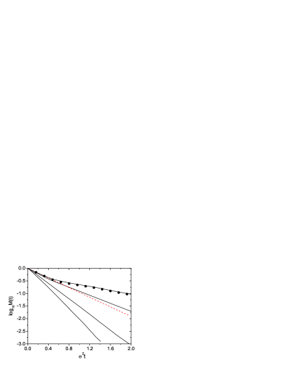
Figure 1: Fidelity $\overline{M}(t)$ as a function of $\sigma^{2}t$ for $K_{0}=0.4$, $\epsilon\approx 7.67\times 10^{-5}$ and $N=N_{0},2N_{0},4N_{0},8N_{0}$ (from bottom to top) where $N_{0}=4096$. ($\sigma=0.05,0.1,0.2,0.4$). The FGR decay $\simeq e^{-2.2\sigma^{2}t}$ is shown by the dashed line. Full circles represent the semiclassical values $\overline{M}_{a}(t)$ at $\sigma=0.4$, computed with expression (7). The numerically computed semiclassical values $\overline{M}_{f}(t)$ turn out to be negligible so that $\overline{M}(t)$ is well approximated by $\overline{M}_{a}(t)$, as clearly seen from the figure at $\sigma=0.4$. Averages were performed over 400 initial point sources, with $\theta_{0}$ taken randomly in the interval $[0,2\pi)$. (The same decaying behaviors are observed for initial Gaussian wavepackets.)

We start by displaying numerical results which strongly deviate from the expected behavior. We consider here the simple, well known, sawtooth map modelBC02 . The classical map writes:

$$\overline{p}=p+K_{0}(\theta-\pi),\ \overline{\theta}=\theta+\overline{p}.\ \ ({\rm mod}\ 2\pi)$$ (2)

For $K_{0}>0$, the motion is completely chaotic, with Lyapunov exponent $\lambda=ln\{(2+K_{0}+[(2+K_{0})^{2}-4]^{1/2})/2\}$. The quantum evolution on one map iteration is described by

$$\overline{\psi}=U_{0}\psi\equiv{\rm exp}\left[-i{\hat{p}}^{2}/(2\hbar)\right]{\rm exp}[ik_{0}(\hat{\theta}-\pi)^{2}/2]\psi,$$ (3)

where $\hat{p}=-i\hbar\partial/\partial\theta$ and $k_{0}=K_{0}/\hbar$, with the effective Planck constant $\hbar=2\pi/N$ and $N$ being the dimension of the Hilbert space. For the perturbed system, $K=K_{0}+\epsilon$ and $k=k_{0}+\sigma$, where $\sigma=\epsilon/\hbar$ and $\epsilon<<K_{0}$.

In Fig. 1 we show the fidelity decay in the expected FGR regime $1/\sqrt{N}\lesssim\sigma\lesssim 1$. In spite of the fact that the classical motion is chaotic, it is clearly seen that the behavior does not obey the FGR which, according to JSB01 ; BC02 , should be $\propto exp(-\Gamma t)$ with $\Gamma\approx 2.2\sigma^{2}$. The same conclusion can be drawn from Fig. 2 where we plot the decay rate $\gamma$ of the fidelity as a function of $\sigma$. Indeed at $K_{0}=0.4$ the decay rate $\gamma$ versus $\sigma$ appears quite different from the quadratic one note .

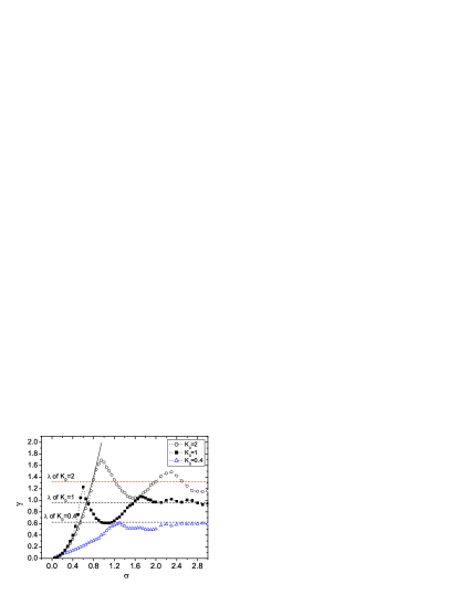
Figure 2: The exponential decay rate $\gamma$ versus perturbation strength $\sigma$, calculated from the best fit of $\ln\overline{M}(t)$. Gaussian wavepackets are taken as initial states. The solid curve shows the rate $\Gamma\simeq 2.2\sigma^{2}$ of the FGR-decay. The dashed horizonal lines correspond to the Lyapunov exponents $\lambda=0.62,0.96$ and 1.32 for $K_{0}=0.4,1$ and 2, respectively. $N=131072$.

Deviations are present even at $K_{0}=1$ and only at $K_{0}=2$ one has good FGR decay. Moreover, above the FGR regime, where one expects Lyapunov decay, there are strong oscillations above and below the decay rate $\lambda$ (for $K_{0}=1$, and $2$). Only at larger $\sigma$ values, one enters the Lyapunov regime.

In order to explain the above numerical results, we start from the standard semiclassical approach JP01 ; VH03 . For simplicity, we consider a finite configuration space, with dimension $d$ and volume ${\cal V}=\int d{\bf r}$. The momentum space is also finite, with a volume ${\cal V}_{p}$. In the semiclassical approach, an initial state $\psi_{0}({\bf r}_{0})$ is propagated by the semiclassical Van Vleck-Gutzwiller propagator, $\psi({\bf r};t)=\int d{\bf r}_{0}K_{\rm sc}({\bf r},{\bf r}_{0};t)\psi_{0}({\bf r}_{0})$, where $K_{\rm sc}({\bf r},{\bf r}_{0};t)=\sum_{s}K_{s}({\bf r},{\bf r}_{0};t)$, with

$$K_{s}({\bf r},{\bf r}_{0};t)=\frac{C_{s}^{1/2}}{(2\pi i\hbar)^{d/2}}{\rm exp}\left[\frac{i}{\hbar}S_{s}({\bf r},{\bf r}_{0};t)-\frac{i\pi}{2}\mu_{s}\right].$$ (4)

The label $s$ in Eq. (4) (more exactly $s({\bf r},{\bf r}_{0};t)$), indicate classical trajectories starting at ${\bf r}_{0}$ and ending at ${\bf r}$ in a time $t$; $S_{s}({\bf r},{\bf r}_{0};t)$ is the time integral of the Lagrangian along the trajectory $s$, $S_{s}({\bf r},{\bf r}_{0};t)=\int_{0}^{t}dt^{\prime}{\cal L}$, $C_{s}=|{\rm det}(\partial^{2}S_{s}/\partial{r_{0i}}\partial r_{j})|$, and $\mu_{s}$ is the Maslov index counting the conjugate points.

In Ref. VH03 , it is shown that the semiclassical approximation to $m(t)$ for initial Gaussian wavepackets has a simple and convenient expression in the initial momentum space. Following similar arguments for initial point sources, $\langle{\bf r}|\Psi_{0}\rangle=\sqrt{(2\pi\hbar)^{d}/{\cal V}_{p}}\delta({\bf r}-{\bf r}_{0})$, ( the theory can be extended to general initial states), one can write $m(t)$ as

$$m({\bf r}_{0},t)\simeq\frac{1}{{\cal V}_{p}}\int d{\bf p}_{0}{\rm exp}\left[\frac{i}{\hbar}\Delta S({\bf p}_{0},{\bf r}_{0};t)\right],$$ (5)

where $\Delta S({\bf p}_{0},{\bf r}_{0};t)$ is the action difference along the trajectory starting at $({\bf r}_{0},{\bf p}_{0})$ for the two systems $H_{0}$ and $H$. In the first order classical perturbation theory, $\Delta S({\bf p}_{0},{\bf r}_{0};t)=\epsilon\int_{0}^{t}dt^{\prime}V[{\bf r}(t^{\prime})]$, with $V$ evaluated along the trajectory.

The averaged (over ${\bf r}_{0}$) fidelity can be separated into a mean-value part and a fluctuating part CLMPV02 , denoted by $\overline{M}_{a}(t)$ and $\overline{M}_{f}(t)$ respectively, $\overline{M}(t)\equiv\overline{|m(t)|^{2}}=\overline{M}_{a}(t)+\overline{M}_{f}(t)$, where

$$\overline{M}_{a}(t)\equiv|\overline{m}(t)|^{2},\ \ {\rm with}\ \ \overline{m}(t)=\frac{1}{\cal V}\int d{\bf r}_{0}m({\bf r}_{0},t).$$ (6)

From Eqs. (5) and (6), it is seen that the mean-value part $\overline{M}_{a}(t)$ can be expressed in terms of the distribution $P(\Delta S)$ of the action difference $\Delta S$,

$$\overline{M}_{a}(t)\simeq\left|\int d\Delta Se^{i\Delta S/\hbar}P(\Delta S)\right|^{2},\hskip 5.69046pt{\rm where}\hskip 39.83368pt$$ (7)

$$P(\Delta S)=\frac{1}{\int d{\bf r}_{0}d{\bf p}_{0}}\int d{\bf r}_{0}d{\bf p}_{0}\delta\left[\Delta S-\Delta S({\bf p}_{0},{\bf r}_{0};t)\right].$$ (8)

It is usually assumed that for chaotic systems $P(\Delta S)$ is close to a Gaussian with a variance $[2\epsilon^{2}K(E)t]$, where $K(E)=\int_{0}^{\infty}dt\langle V[{\bf r}(t)]V[({\bf r}(0)]\rangle$ is the classical action diffusion constant CT02 . As a result, $\overline{M}_{a}(t)\simeq e^{-\Gamma t}$, where $\Gamma=2\sigma^{2}K(E)$. At small $\sigma$, the fluctuation is small compared with the average value, because the phase on the right hand side of Eq. (5) is proportional to $\sigma$; then, $\overline{M}(t)\simeq\overline{M}_{a}(t)$ has the FGR-decay.

Let us now consider a fixed ${\bf r}_{0}$, and divide the space of the initial momenta ${\bf p}_{0}$ into connected, disjoint subspaces, denoted by ${\cal A}_{\alpha}$, where each ${\cal A}_{\alpha}$ is the largest possible subspace such that the correspondence between ${\bf p}_{0}$ and the final position ${\bf r}$ is one-to-one, i.e. different ${\bf p}_{0}$ inside each single component ${\cal A}_{\alpha}$ gives different final position ${\bf r}$. It is always possible to make such a division. The number of subspaces ${\cal A}_{\alpha}$ is denoted by $N_{\alpha}$. Note also that the sizes of ${\cal A}_{\alpha}$ decrease exponentially with increasing time $t$. When ${\bf p}_{0}$ runs over a subspace ${\cal A}_{\alpha}$, ${\bf r}$ may run over part of the configuration space, denoted by ${\cal V}_{\alpha}$. Note that, with this division of the ${\bf p}_{0}$ subspace, the trajectories starting at ${\bf r}_{0}$ are divided into $N_{\alpha}$ groups and “near” trajectories typically belong to the same group.

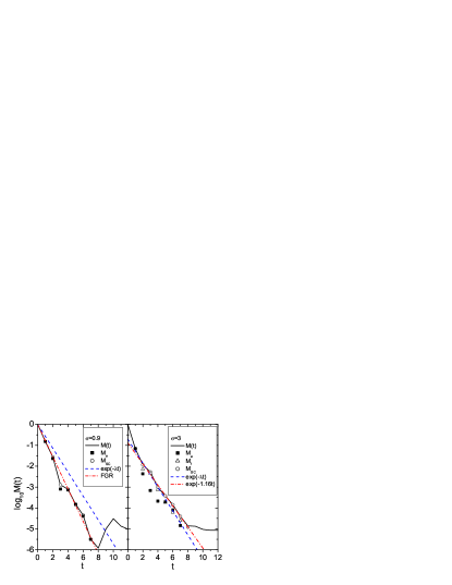
Figure 3: Comparison between the exact $\overline{M}(t)$, its semiclassical mean-value part $\overline{M}_{a}$, calculated by using Eqs. (5) and (6), and the fluctuation part $\overline{M}_{f}=\overline{M}_{\rm sc}-\overline{M}_{a}$, where $\overline{M}_{\rm sc}$ is the semiclassical approximation to the fidelity, computed by the expression (5). Here $N=131072$, $K_{0}=2$, and $\sigma=0.9$ (left panel), $\sigma=3$(right panel). The exact $\overline{M}(t)$ is in good agreement with its semiclassical approximation $\overline{M}_{\rm sc}(t)$. The average is taken over 500 initial point sources.

The amplitude $m({\bf r}_{0},t)$ in Eq. (5) can now be written as $m({\bf r}_{0},t)\simeq\sum_{\alpha}m_{\alpha}({\bf r}_{0},t)$, where

$$m_{\alpha}({\bf r}_{0},t)=\frac{1}{{\cal V}_{p}}\int_{{\cal V}_{\alpha}}d{\bf r}C_{s}{\rm exp}\left[\frac{i}{\hbar}\Delta S_{s}({\bf r},{\bf r}_{0};t)\right]$$ (9)

with integration over the subspace ${\cal V}_{\alpha}$, in which the change of variable ${\bf p}_{0}\to{\bf r}$ within the subspaces ${\cal A}_{\alpha}$ has been done and $\Delta S_{s}({\bf r},{\bf r}_{0};t)$ coincides with $\Delta S({\bf p}_{0},{\bf r}_{0};t)$ for the same trajectory $s$ starting at $({\bf r}_{0},{\bf p}_{0})$ with ${\bf p}_{0}\in{\cal A}_{\alpha}$. $\overline{M}_{f}(t)$ is written as

$$\overline{M}_{f}(t)\simeq\overline{\left|\sum_{\alpha}m_{\alpha f}\right|^{2}}\hskip 2.84544pt{\rm with}\ m_{\alpha f}=m_{\alpha}({\bf r}_{0},t)-\frac{\overline{m}(t)}{N_{\alpha}}.$$ (10)

When $\sigma$ is large enough, above a critical border $\sigma_{f}$, $m_{\alpha}({\bf r}_{0},t)$ can be regarded as possessing random phase, and therefore $\overline{M}_{f}$ can be approximated by its diagonal part

$$\overline{M}_{f}(t)\simeq\overline{\sum_{\alpha}|m_{\alpha f}|^{2}}\simeq\overline{\sum_{\alpha}|m_{\alpha}({\bf r}_{0},t)|^{2}}\hskip 56.9055pt$$

$$\propto\int d{\bf r}_{0}\sum_{\alpha}\left|\int_{{\cal V}_{\alpha}}d{\bf r}C_{s}{\rm exp}\left(\frac{i}{\hbar}\Delta S_{s}\right)\right|^{2},$$ (11)

where the second approximation is obtained by noticing that $|\overline{m}(t)/N_{\alpha}|<<|m_{\alpha}|$ at large $\sigma$.

When the phase space is homogeneous with constant local (maximum) Lyapunov exponent $\lambda$, as in the sawtooth map, the number $N_{s}({\bf r}_{0},{\bf r})$ of trajectories connecting two points ${\bf r}_{0}$ and ${\bf r}$ in the configuration space is approximately $N_{s}\simeq N_{\alpha}\simeq e^{\lambda t}$Haake . The summation over $\alpha$ in (11) gives a contribution approximately proportional to $N_{s}$. At $t$ large enough, the main time dependence of $|\int_{{\cal V}_{\alpha}}d{\bf r}C_{s}e^{\frac{i}{\hbar}\Delta S_{s}}|$ is given by $C_{s}\propto e^{-\lambda t}$. Combining these results, it is seen that at $\sigma>\sigma_{f}$, $\overline{M}_{f}(t)$ has the Lyapunov decay, $\overline{M}_{f}(t)\propto e^{-\lambda t}$.

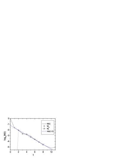
Figure 4: Similar to Fig. 3, for $K_{0}=1$ and $\sigma=6$. At this large $\sigma$, $\overline{M}_{a}(t)$ is negligible compared with $\overline{M}_{f}(t)$.

In order to have the Lyapunov decay for $\overline{M}(t)$, the term $\overline{M}_{a}(t)$ must be small. To this end one needs to further increase $\sigma$ above a critical value $\sigma_{r}$, so that the variance of the phase of $m({\bf r}_{0},t)$ with respect to ${\bf r}_{0}$ will become so large that $\overline{M}_{a}(t)$ is negligible.

The right panel of Fig. 3 gives an example of $\overline{M}_{a}(t)\approx\overline{M}_{f}(t)$. This explains the fluctuation of $\gamma$ versus $\sigma$ shown in Fig. 2 at $K_{0}=2$ and $\sigma<3$. Fig. 4 instead gives an example with $\sigma$ large enough ($\sigma>\sigma_{r}$), so that $\overline{M}_{a}(t)$ is negligible and $\overline{M}(t)\simeq\overline{M}_{f}(t)$.

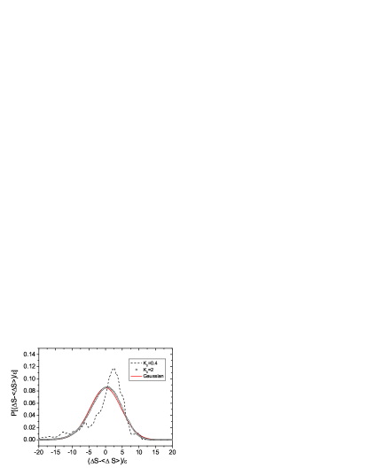
Figure 5: Distribution $P[(\Delta S-\langle\Delta S\rangle)/\epsilon]$ of the classical action difference $\Delta S$, at $t=10$, calculated by taking randomly $10^{7}$ initial points in the phase space, where $\langle\Delta S\rangle\equiv\epsilon t\langle V(\theta)\rangle=-\pi^{2}\epsilon t/6$, with an average over the phase space.

The deviation from FGR decay observed in Figs. 1 and 2 is due to the deviation of $P(\Delta S)$ from the Gaussian behavior. Indeed, when chaos in the underlying classical dynamics is strong enough ($K_{0}>1$), correlations between non-overlapping parts of a trajectory decay very rapidly and the distribution $P(\Delta S/\epsilon)$ reaches, in a relatively short time, the Gaussian distribution. This is the case of Fig. 5 for $K_{0}=2$ , where $K(E)=\pi^{4}/90\simeq 1.08$ with $\Gamma=2K(E)\sigma^{2}\simeq 2.16\sigma^{2}$, in agreement with the numerical results in Ref. BC02 and in Fig. 2. However, when $K_{0}$ is not sufficiently large, e.g., $K_{0}=0.4$, a considerable deviation of $P(\Delta S/\epsilon)$ from the Gaussian distribution appears for times comparable to the fidelity decay times (Fig. 5). According to Eq. (7), this leads to deviations from the FGR-decay as observed in Fig. 1. We would like to draw the reader attention to the fact that, for $K_{0}<1$ the saw-tooth map, even though completely chaotic, it possess a structure of cantori which, in the quantum case, can act as perfect barriers to quantum motion thus leading to localization of wavefunctions.

Notice that the deviation of $P(\Delta S/\epsilon)$ from the Gaussian distribution depends on $K_{0}$ but not on $\epsilon$ or $\sigma$. Therefore, by increasing $\sigma$, the effect of this deviation becomes more and more important, since the FGR exponential decay has a decay rate proportional to $\sigma^{2}$ while the deviation from the Gaussian remains unchanged. Therefore, for a given system, there is a critical value $\sigma_{d}$, below which the FGR decay is obeyed with good accuracy and above which FGR breaks down. This case is illustrated in Fig. 2 for the case $K_{0}=1$, which coincides with the well-known Arnold cat map, the paradigmatic model of chaos. Here the distribution $P(\Delta S/\epsilon)$ (at t= 10) is slightly different from the Gaussian distribution and the decay rate $\gamma$ of fidelity deviates from the FGR decay for $\sigma\gtrsim 0.3$. In cases of weak classical chaos, the value of $\sigma_{d}$ can be so small that FGR is never observed (e.g. the case with $K_{0}=0.4$). The left panel in Fig. 3 shows instead a case at $K_{0}=2$ and $\sigma=0.9$, in which $\overline{M}_{a}(t)$ obeys the FGR decay and $\overline{M}_{f}(t)$ is negligible.

To summarize: above the perturbative border, the fidelity has a FGR decay for $\sigma<\sigma_{d}$, while for $\sigma>\sigma_{r}$, it has the Lyapunov decay. In the intermediate region, for $\sigma_{d}<\sigma<\sigma_{f}$, the fidelity deviates from FGR and can decay even faster than Lyapunov. For $\sigma_{f}<\sigma<\sigma_{r}$, $\overline{M}_{a}(t)\sim\overline{M}_{f}(t)$ and the decay rate of $\overline{M}(t)$ fluctuates around the Lyapunov exponent. It may be useful to recall here the physical meaning of different borders. Above $\sigma_{d}$, the distribution $P(\Delta S)$ deviates from the Gaussian and this induces deviations from the expected FGR decay. Below $\sigma_{r}$, $\overline{M}_{a}(t)$ is non negligible as compared to $\overline{M}_{f}(t)$ and this induces deviations from the expected Lyapunov decay.

It may be interesting to remark that the relation between the decomposition in two part of $\overline{M}(t)$ here and that in Ref. JP01 is the following. At $\sigma$ small enough $\overline{M}(t)\simeq\overline{M}_{a}(t)\simeq M^{nd}(t)$, with $\overline{M}_{f}(t)$ and $M^{d}(t)$ negligible; while at $\sigma$ large enough $\overline{M}(t)\simeq\overline{M}_{f}(t)\simeq M^{d}(t)$, with $\overline{M}_{a}(t)$ and $M^{nd}(t)$ negligible. In the intermediate regime of $\sigma$, in particular, in the crossover from the FGR decay to the Lyapunov decay, there may be considerable difference between the two divisions.

In this paper, by using the sawtooth map, we have demonstrated that the fidelity decay in a generic chaotic system can have a very complex behavior. In particular, deviations from the Fermi golden rule (for weak chaos) and Lyapunov decay have been discussed as well as the existence of perturbation borders separating different regimes. It is our opinion that fidelity is an important quantity which characterizes the stability of classical and quantum systems. It therefore deserves deeper analytical and numerical studies in order to fully understand its behavior in different dynamical regimes.

The authors are grateful to V. Sokolov for valuable discussions. This work was supported in part by the Academic Research Fund of the National University of Singapore. Support was also given by the EC RTN contract HPRN-CT-2000-0156, the NSA and ARDA under ARO contracts No. DAAD19-02-1-0086, the project EDIQIP of the IST-FET programme of the EC, the PRIN-2002 “Fault tolerance, control and stability in quantum information processing”, and the Natural Science Foundation of China No.10275011.

References

(1) A. Peres, Phys. Rev. A 30, 1610 (1984).
(2) T. Prosen, Phys. Rev. E 65, 036208 (2002);
T. Prosen and M. Žnidarič, J. Phys. A 35, 1455 (2002).
(3) N. R. Cerruti and S. Tomsovic, Phys. Rev. Lett. 88,
054103 (2002); J. Phys. A 36, 3451 (2003).
(4) Ph. Jacquod, P.G. Silvestrov, and C.W.J. Beenakker,
Phys. Rev. E 64, 055203 (2001).
(5) Ph. Jacquod, I. Adagideli, and C.W.J. Beenakker,
Phys. Rev. Lett. 89, 154103 (2002).
(6) J. Emerson et al., Phys. Rev. Lett. 89, 284102 (2002).
(7) R.A. Jalabert and H.M. Pastawski,Phys. Rev. Lett. 86,
2490 (2001).
(8) F.M. Cucchietti, H.M. Pastawski, and D.A. Wisniacki, Phys. Rev. E 65,
045206 (2002);
(9) D.A. Wisniacki and D. Cohen, Phys. Rev. E 66, 046209 (2002).
(10)D.A. Wisniacki et al., Phys. Rev. E 65, 055206 (2002);
(11) F.M. Cucchietti et al., Phys. Rev. E 65, 046209 (2002).
(12) G. Benenti and G. Casati, Phys. Rev. E 65,
066205(2002); F. Borgonovi, G. Casati, and B. Li, Phys. Rev. Lett. 77, 4744 1996).
(13) W.G. Wang and B. Li, Phys. Rev. E 66, 056208 (2002).
(14) J. Vaníček and E. Heller, Phys. Rev. E 68, 056208 (2003).
(15)F. M. Cucchietti et al quant-ph/0307752.
(16) Deviations from Fermi golden rule have also been observed
in the Bunimovich stadium billiard Wis02 .
The fidelity in that model was found to decay as ,
with being the half width of the LDOS.
In our case the decay rate of fidelity is close to .
However, for considerable deviations in tail region of LDOS from the Lorentzian shape are present.
(17) F. Haake, Quantum Signatures of Chaos, 2nd ed.
(Springer-Verlag, Berlin, 2001).