Exploiting entanglement in communication channels with correlated noise

Abstract

We develop a model for a noisy communication channel in which the noise affecting consecutive transmissions is correlated. This model is motivated by fluctuating birefringence of fiber optic links. We analyze the role of entanglement of the input states in optimizing the classical capacity of such a channel. Assuming a general form of an ensemble for two consecutive transmissions, we derive tight bounds on the classical channel capacity depending on whether the input states used for communication are separable or entangled across different temporal slots. This result demonstrates that by an appropriate choice, the channel capacity may be notably enhanced by exploiting entanglement.

I Introduction

Entanglement is a fragile feature of composite quantum systems that can easily diminish by uncontrollable interactions with the environment. At the same time however carefully crafted entangled states can protect quantum coherence from the deleterious effects of those random interactions. This idea underlies the principles of quantum error correcting codes that strengthen the optimism regarding the feasibility of implementing in practice complex quantum information processing tasks NielsenChuang .

In this paper we demonstrate how quantum entanglement can help in the task of classical communication. To this end, we develop a simple model of a noisy communication channel, where the noise affecting consecutive transmissions is correlated. Within this model, we derive bounds on the classical channel capacity assuming either separable or entangled input states, and we show that using collective entangled states of transmitted particles leads to an enhanced capacity of the channel.

The motivation for our model comes from classical fiber optic communications GhatakThyagarajan . In practice, light transmitted through a fiber optic link undergoes a random change of polarization induced by the birefringence of the fiber. The fiber birefringence usually fluctuates depending on the environmental conditions such as temperature and mechanical strain. At first sight, this makes the polarization degree of freedom unsuitable for encoding information, as the input polarization state gets scrambled on average to a completely mixed state. However, the birefringence fluctuations have a certain time constant which means that the transformation of the polarization state, though random, remains nearly the same on short time scales. Consider now sending a pair of photons whose temporal separation lies well within this time scale. Although the polarization state of each one of the photons when looked at separately becomes randomized, certain properties of the joint state remain preserved. For example, this is the case of the relative polarization of the second photon with respect to the first one. We can therefore try to decode from the output whether the input polarizations were mutually parallel or orthogonal. This property cannot be determined perfectly, as in general we cannot tell whether two general quantum states are identical or orthogonal if we do not know anything else about them KashKentPRA02 , but even the ability of providing a partial answer establishes correlations between the channel input and output that can be used to encode information into the polarization degree of freedom. The situation becomes even more interesting when we allow for entangled quantum states. Then the singlet polarization state of the two photons, when sent as the input, remains invariant under such perfectly correlated depolarization, and it can be discriminated unambiguously against the triplet subspace. Therefore we can encode one bit of information into the polarization state of two photons by sending either a singlet state or any of the triplet states. We shall see that these simple observations will also emerge from our general analysis of the channel capacity.

The first example of entanglement-enhanced information transmission over a quantum channel with correlated noise has been recently analyzed by Macchiavello and Palma MaccPalmPRA02 . Our model assumes a different form of correlations, and its high degree of symmetries has allowed us to perform optimization of the channel capacity over arbitrary input ensembles. Although we analyze only zero- and one-photon signals, we define the action of the channel in terms of the transformations of the bosonic annihilation operators, which sets up a framework for possible generalizations, such as use of multiphoton signals. This application of entanglement in classical communication is a distinct problem from entanglement-assisted classical capacity of noisy quantum channels studied by Bennett et al. in Ref. BennShorPRL99 , where it has been shown that prior entanglement shared between sender and receiver can increase the classical capacity. We also note that the non-zero time constant of phase and polarization fluctuations can be used in robust protocols for long-haul quantum key distribution WaltAbouPRL03 ; BoilGootXXX03 .

Before passing on to a detailed discussion of the problem in the subsequent sections, let us introduce some basic notation. The action of a channel is described by a completely positive map HausJozsPRA96 that we will denote by $\Lambda(\cdot)$. The sender selects messages from an input ensemble $\{p_{i},\hat{\varrho}_{i}\}$, where $p_{i}$ is the probability of sending the state $\hat{\varrho}_{i}$ through the channel. The capacity of the channel is a function of the mutual information between the input ensemble and measurement outcomes at the receiving stations: it characterizes the strength of correlations between these two that are preserved by the channel. The mutual information itself involves a specific measurement scheme; however, it has a very useful upper bound in the form of the Holevo quantity that depends only on the output ensemble of states $\{p_{i},\Lambda(\hat{\varrho}_{i})\}$ emerging from the channel Holevo :

$$\chi=S\left(\sum_{i}p_{i}\Lambda(\hat{\varrho}_{i})\right)-\sum_{i}p_{i}S(\Lambda(\hat{\varrho}_{i}))$$ (1)

where $S$ is the von Neumann entropy $S(\hat{\varrho})=-\text{Tr}(\hat{\varrho}\log_{2}\hat{\varrho})$. As we will see, in our model the Holevo quantity will provide a tight bound on the mutual information that could be achieved in practice using a simple measurement scheme. The classical channel capacity is obtained by assuming arbitrarily long sequences of possibly entangled input systems, and calculating the average capacity per single use of the channel. In our analysis, we will perform a restricted optimization by considering only two consecutive uses of the channel.

II Channel decomposition

We will start our discussion by proving a rather general lemma about channels that can be decomposed into a direct sum of maps acting on subspaces of the Hilbert space of the input systems. In physical terms, such channels remove quantum coherence between the components of the input state that belong to different subspaces, by zeroing the respective off-diagonal blocks of the density matrix characterizing the input state. This lemma will greatly simplify our further calculations.

Lemma 1: Suppose that we can decompose the Hilbert space ${\cal H}$ of the system into a direct sum of subspaces

$${\cal H}=\bigoplus_{k}{\cal H}^{(k)}$$ (2)

such that for an arbitrary input state $\hat{\varrho}$ the state emerging from the channel $\Lambda(\hat{\varrho})$ can be represented as

$$\Lambda({\hat{\varrho}})=\bigoplus_{k}\Lambda^{(k)}(\hat{\varrho}^{(k)})$$ (3)

where $\hat{\varrho}^{(k)}={\hat{\varrho}}|_{{\cal H}^{(k)}}$ is the input state $\hat{\varrho}$ truncated to the subspace ${\cal H}^{(k)}$, and each $\Lambda^{(k)}$ is a certain trace-preserving completely positive map acting in the corresponding subspace ${\cal H}^{(k)}$. Then the optimal channel capacity can be attained with an ensemble in which each state belongs to one of the subspaces ${\cal H}^{(k)}$.

Proof: Indeed, suppose that there is a state $\hat{\varrho}$ that does not satisfy the above condition, i.e. it is defined on more that one subspace ${\cal H}^{(k)}$. We can replace it by a sub-ensemble $\{\text{Tr}(\hat{\varrho}^{(k)});\hat{\varrho}^{(k)}/\text{Tr}(\hat{\varrho}^{(k)})\}$, obtained by truncating the state $\hat{\varrho}$ to the subspaces ${\cal H}^{(k)}$ and normalizing the resulting density matrices. In other words, whenever the sender is supposed to transmit $\hat{\varrho}$, she replaces it by one of the normalized truncated states $\hat{\varrho}^{(k)}/\text{Tr}(\hat{\varrho}^{(k)})$ with the corresponding probability $\text{Tr}(\hat{\varrho}^{(k)})$. It is straightforward to verify that the average state obtained from such a subensemble is identical with $\Lambda(\hat{\varrho})$.

The above observation has a useful consequence when optimizing the Holevo bound on channel capacity. If the input ensemble is of the form discussed above, then it can be split into subensembles of states that belong to separate subspaces ${\cal H}^{(k)}$, with the probability distributions normalized to one within each subensemble, and $p_{k}$ denoting the probability of sending a state from the $k$th subensemble. It is then easy to check that the Holevo quantity is given by the following expression:

$$\chi=\sum_{k}p_{k}\chi^{(k)}-\sum_{k}p_{k}\log_{2}p_{k},$$ (4)

where $\chi^{(k)}$ is the Holevo quantity for the $k$th subensemble. Therefore, the maximization of the Holevo quantity can be performed in two steps. The first one is the optimization of each of $\chi^{(k)}$ separately, assuming an input ensemble restricted to the subspace ${\cal H}^{(k)}$. The second step consists of optimizing the probability distribution $p_{k}$ with the normalization constraint $\sum_{k}p_{k}=1$, and it can be performed explicitly using the method of Lagrange multipliers. Indeed, if we denote the Lagrange multiplier as $\lambda$, then differentiation over $p_{l}$ yields:

$$0=\frac{\partial}{\partial p_{l}}\left(\chi-\lambda\sum_{k}p_{k}\right)=\chi^{(l)}-\log_{2}p_{l}-\frac{1}{\ln 2}-\lambda.$$ (5)

This formula allows us to express the probabilities $p_{l}$ in terms of the Lagrange multiplier $\lambda$ as:

$$p_{l}=2^{\chi^{(l)}-1/\ln 2-\lambda},$$ (6)

and furthermore summation over $l$ and using the fact that $\sum_{l}p_{l}=1$ gives the value of the Lagrange multiplier as:

$$\lambda=\log_{2}\left(\sum_{l}2^{\chi^{(l)}}\right)-\frac{1}{\ln 2}.$$ (7)

Finally, inserting Eqs. (6) and (7) into Eq. (4) yields the maximum value of the Holevo quantity equal to:

$$\chi=\log_{2}\left(\sum_{k}2^{\chi^{(k)}}\right).$$ (8)

We will later find this expression useful in calculating the channel capacity in our model. The physical reason for this is that we will be able to decompose the set of states used for communication into subensembles with a fixed number of photons, and then optimize the Holevo quantity separately in each subspace.

III Depolarization model

Let us now introduce a mathematical model for the random transformation of polarization during transmission through the channel. A general linear transformation between two annihilation operators corresponding to a pair of orthogonal modes is given by $2\times 2$ unitary matrices CampSalePRA89 that form the Lie group U(2). In situations when only the relative phase between the two polarization modes is relevant, the overall phase of the transformation can be assumed to be fixed, which reduces the group of transformations to SU(2). However, in our case the overall phase shift can vary between the consecutive temporal slots, and therefore we need to keep it as an independent parameter. We note that any U(2) matrix can be mapped onto a rotation in the three dimensional physical space. Such a rotation describes the corresponding transformation of the Poincaré sphere used to represent the polarization state of light in classical optics BornWolf . We will label elements of U(2) as ${\bf\Omega}$ and use a dot to denote the multiplication within the group. The U(2) group has a natural invariant integration measure which we assume is normalized to one $\int\text{d}{\bf\Omega}=1$. This measure defines a uniformly randomized distribution of polarization transformations that scrambles an arbitrary input polarization to a completely mixed one.

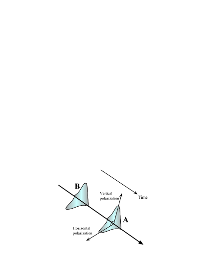
Figure 1: Representation of two consecutive temporal slots labelled by $A$ and $B$. The Hilbert space of each slot is spanned in our model by three states: the zero-photon state $|0\rangle$ and two mutually orthogonal polarization states denoted by $|\leftrightarrow\rangle$ and $|\updownarrow\rangle$.

Suppose now that two consecutive temporal slots labelled by $A$ and $B$, each comprising two orthogonal polarizations, are occupied by a joint state of radiation $\hat{\varrho}_{AB}$, as shown schematically in Fig. 1. We will assume that the polarization transformation ${\bf\Omega}_{A}$ affecting the slot $A$ is completely random, but that the transformation ${\bf\Omega}_{B}$ is correlated with the first one through a conditional probability distribution $p({\bf\Omega}_{B}|{\bf\Omega}_{A})$. The resulting transformation of the joint two-slot state is therefore given by the following completely positive map:

$$\Lambda(\hat{\varrho}_{AB}) = \int d{\bf\Omega}_{A}\int d{\bf\Omega}_{B}\,p({\bf\Omega}_{B}|{\bf\Omega}_{A})$$

$$\times\hat{U}({\bf\Omega}_{A})\otimes\hat{U}({\bf\Omega}_{B})\,\hat{\varrho}_{AB}\,\hat{U}^{\dagger}({\bf\Omega}_{A})\otimes\hat{U}^{\dagger}({\bf\Omega}_{B}).$$

Here $\hat{U}({\bf\Omega})$ is a unitary matrix acting in the Hilbert space of one of the slots that represents the polarization transformation ${\bf\Omega}$. We will now assume that the conditional probability $p({\bf\Omega}_{B}|{\bf\Omega}_{A})$ depends only on the relative transformation between the slots $A$ and $B$ and that it can consequently be represented as $p({\bf\Omega}_{B}|{\bf\Omega}_{A})=p({\bf\Omega}_{B}\cdot{\bf\Omega}_{A}^{-1})$. In such a case, we can substitute the integration variables in the second integral according to ${\bf\Omega}_{B}={\bf\Omega}^{\prime}\cdot{\bf\Omega}_{A}$, and make use of the invariance of the integration measure $\text{d}{\bf\Omega}_{B}=\text{d}{\bf\Omega}^{\prime}$. This procedure shows that the map $\Lambda$ can be represented as a composition of two maps: $\Lambda=(\hat{\openone}\otimes\Lambda_{\text{dep}})\circ\Lambda_{\text{perf}}$. The first one of them, $\Lambda_{\text{perf}}$, acts on both the temporal slots and it depolarizes them in exactly the same way:

$$\Lambda_{\text{perf}}(\hat{\varrho}_{AB})=\int d{\bf\Omega}\,\hat{U}({\bf\Omega})\otimes\hat{U}({\bf\Omega})\,\hat{\varrho}_{AB}\,\hat{U}^{\dagger}({\bf\Omega})\otimes\hat{U}^{\dagger}({\bf\Omega})$$ (10)

The second map, $\Lambda_{\text{dep}}$, acts only on the slot $B$, and it introduces additional depolarization relative to the slot $A$ according to the probability distribution $p({\bf\Omega}^{\prime})$:

$$\Lambda_{\text{dep}}(\hat{\varrho}_{B})=\int d{\bf\Omega}^{\prime}\,p({\bf\Omega}^{\prime})\hat{U}({\bf\Omega}^{\prime})\hat{\varrho}_{B}\hat{U}^{\dagger}({\bf\Omega}^{\prime}).$$ (11)

We will assume later that the distribution $p({\bf\Omega}^{\prime})$ has sufficient symmetry to describe the action of the map $\Lambda_{\text{dep}}$ in the relevant Hilbert space with the help of two simple parameters.

We now introduce a further simplification by imposing a condition that each temporal slot may contain at most one photon. Therefore the relevant Hilbert space for each slot is spanned by three states: the zero-photon state $|0\rangle$, and horizontally and vertically polarized one-photon states $|\leftrightarrow\rangle$ and $|\updownarrow\rangle$. We can conveniently write the explicit form of the unitary transformation $\hat{U}({\bf\Omega})$ using the irreducible unitary representations of the group SU(2). We will denote by $\hat{\cal D}^{j}({\bf\Omega})$ a $(2j+1)\times(2j+1)$ matrix that is a $(2j+1)$-dimensional representation of an SU(2) element obtained from ${\bf\Omega}$ by fixing the overall phase factor to one. These matrices are well known in the quantum theory of angular momentum as describing transformations of a spin-$j$ particle under the rotation group BrinkSatchler . We will also denote by $\alpha({\bf\Omega})$ the overall phase of the element ${\bf\Omega}$. Then the unitary transformation of the input state corresponding to the polarization rotation ${\bf\Omega}$ is given by the matrix:

$$\hat{U}({\bf\Omega})=\left(\begin{array}[]{cc}\hat{\cal D}^{0}({\bf\Omega})&\begin{array}[]{cc}0&0\end{array}\\ \begin{array}[]{c}0\\ 0\end{array}&e^{i\alpha({\bf\Omega})}\hat{\cal D}^{1/2}({\bf\Omega})\end{array}\right).$$ (12)

In this formula, the one-dimensional representation $\hat{\cal D}^{0}({\bf\Omega})$ is identically equal to one, and $e^{i\alpha({\bf\Omega})}\hat{\cal D}^{1/2}({\bf\Omega})$ is a $2\times 2$ unitary matrix itself; however, we will keep this more general notation in order to be able to use results from the theory of group representations. In particular, the following property of the rotation matrix elements will allow us to evaluate directly a number of expressions:

$$\int\text{d}{\bf\Omega}[{\cal D}^{j}_{mn}({\bf\Omega})]^{\ast}{\cal D}^{j^{\prime}}_{m^{\prime}n^{\prime}}({\bf\Omega})=\frac{1}{2j+1}\delta_{jj^{\prime}}\delta_{mm^{\prime}}\delta_{nn^{\prime}}.$$ (13)

The action of the map $\Lambda_{\text{perf}}$ on a joint two-slot state can be analyzed most easily if we decompose the complete Hilbert space into a direct sum of subspaces with a fixed number of photons: ${\cal H}={\cal H}^{(0)}\oplus{\cal H}^{(1)}\oplus{\cal H}^{(2)}$, where the upper index labels the number of photons. The zero-photon subspace is spanned by a single state $|0_{A}0_{B}\rangle$. The one-photon space has a basis formed by four vectors: $|\leftrightarrow_{A}0_{B}\rangle$, $|\updownarrow_{A}0_{B}\rangle$, $|0_{A}\leftrightarrow_{B}\rangle$, and $|0_{A}\updownarrow_{B}\rangle$. Finally, in the two-photon subspace ${\cal H}^{(2)}$ we will introduce a basis that consists of the singlet state $|\Psi_{-}\rangle=(|\leftrightarrow_{A}\updownarrow_{B}\rangle-|\updownarrow_{A}\leftrightarrow_{B}\rangle)/\sqrt{2}$ and the three triplet states $|\leftrightarrow_{A}\leftrightarrow_{B}\rangle$, $|\Psi_{+}\rangle=(|\leftrightarrow_{A}\updownarrow_{B}\rangle+|\updownarrow_{A}\leftrightarrow_{B}\rangle)/\sqrt{2}$, and $|\updownarrow\rangle_{A}\updownarrow\rangle_{B}$. The reason for this choice is that then the action of the tensor product $\hat{\cal D}^{1/2}({\bf\Omega})\otimes\hat{\cal D}^{1/2}({\bf\Omega})$ on a two-photon state can be decomposed into the sum: $\hat{\cal D}^{1/2}({\bf\Omega})\otimes\hat{\cal D}^{1/2}({\bf\Omega})=\hat{\cal D}^{0}({\bf\Omega})\oplus\hat{\cal D}^{1}({\bf\Omega})$ where $\hat{\cal D}^{0}({\bf\Omega})$ acts on the singlet state $|\Psi_{-}\rangle$, and $\hat{\cal D}^{1}({\bf\Omega})$ is a three-dimensional matrix acting in the triplet subspace. Using our decomposition of the complete Hilbert space, the action of the tensor product $\hat{U}({\bf\Omega})\otimes\hat{U}({\bf\Omega})$ on a general two-slot state in the basis specified above is given by:

$$\hat{U}({\bf\Omega})\otimes\hat{U}({\bf\Omega})=\hat{\cal D}^{0}({\bf\Omega})\oplus e^{i\alpha({\bf\Omega})}\left(\begin{array}[]{cc}\hat{\cal D}^{1/2}({\bf\Omega})&\begin{array}[]{cc}0&0\\ 0&0\end{array}\\ \begin{array}[]{cc}0&0\\ 0&0\end{array}&\hat{\cal D}^{1/2}({\bf\Omega})\end{array}\right)\oplus e^{2i\alpha({\bf\Omega})}\left(\begin{array}[]{cc}\hat{\cal D}^{0}({\bf\Omega})&\begin{array}[]{ccc}0&0&0\end{array}\\ \begin{array}[]{c}0\\ 0\\ 0\end{array}&\hat{\cal D}^{1}({\bf\Omega})\end{array}\right)$$ (14)

If we now insert this fomula into Eq. (10), it can be easily seen that the invariant integration over the overall phase factor $\alpha({\bf\Omega})$ kills all the off-block diagonal elements of the density matrix that link different subspaces ${\cal H}^{(k)}$. In other words, all the coherence between states with different photon numbers is completely removed by the phase fluctuations. Furthermore, the operation $\Lambda_{\text{dep}}$, acting only on the second slot, does not mix subspaces with different photon numbers. Therefore the conditions of our lemma are satisfied and we can consider only states with a definite number of photons as elements of the input ensemble. Thus we need to calculate are three corresponding Holevo quantities $\chi^{(0)}$, $\chi^{(1)}$, and $\chi^{(2)}$ that can be combined into a Holevo bound for the overall channel capacity according to Eq. (8). This calculation forms the contents of the next section.

IV Channel capacity

The communication capacity $\chi^{(0)}$ of the zero-photon subspace itself ${\cal H}^{(0)}$ is naturally zero, as we have only a single state $|0_{A}0_{B}\rangle$ at our disposal. This state can of course be used as an element of a larger ensemble thus contributing to the overall capacity. This fact is reflected in the form of Eq. (8), where $\chi^{(0)}=0$ indeed does increase the total value of $\chi$.

IV.1 One-photon subspace

A less trivial problem to calculate is the capacity of the one-photon subspace. If we assume a normalized input state $\hat{\varrho}_{\text{in}}$ from the subspace ${\cal H}^{(1)}$, then the action of the channel $\Lambda_{\text{perf}}$ restricted to this subspace is given by:

$$\Lambda^{(1)}_{\text{perf}}(\hat{\varrho}_{\text{in}})=\frac{1}{2}\left(\begin{array}[]{cccc}a&0&b&0\\ 0&a&0&b\\ b^{\ast}&0&1-a&0\\ 0&b^{\ast}&0&1-a\end{array}\right)$$ (15)

where the parameters $a$ and $b$ are defined in terms if the input density matrix as:

$$a = \langle\leftrightarrow_{A}0_{B}|\hat{\varrho}_{\text{in}}|\leftrightarrow_{A}0_{B}\rangle+\langle\updownarrow_{A}0_{B}|\hat{\varrho}_{\text{in}}|\updownarrow_{A}0_{B}\rangle$$

$$b = \langle\leftrightarrow_{A}0_{B}|\hat{\varrho}_{\text{in}}|0_{A}\leftrightarrow_{B}\rangle+\langle\updownarrow_{A}0_{B}|\hat{\varrho}_{\text{in}}|0_{A}\updownarrow_{B}\rangle$$ (16)

For the form of density matrix given in Eq. (15), the depolarizing channel $\Lambda_{\text{dep}}$ affects only the off-diagonal elements $b$ and $b^{\ast}$. We will assume that the symmetry of the distribution $p({\bf\Omega}^{\prime})$ is such that the effect of $\Lambda_{\text{dep}}$ is a rescaling of these elements by a real parameter $\eta^{\prime}$ bounded between $0$ and $1$. It is now easy to check that the entropy of the one-photon state emerging from the channel can be written as

$$S(\Lambda(\hat{\varrho}_{\text{in}}))=1+S(\left(\begin{array}[]{cc}a&\eta^{\prime}b\\ \eta^{\prime}b^{\ast}&1-a\end{array}\right))$$ (17)

where the $2\times 2$ matrix appearing in the second term can be interpreted as a state of a qubit. Therefore, the second term is bounded by $0$ and $1$, and consequently $1\leq S(\Lambda(\hat{\varrho}_{\text{in}}))\leq 2$. It is a straightforward observation that the Holevo quantity is bound from above by the difference between the maximum and the minimum possible entropies of states emerging from the channel. Therefore we obtain that $\chi^{(1)}\leq 1$. This inequality can be saturated simply by taking a one-photon state confined either to the first or to the second temporal slot, with an arbitrary polarization. Thus, the channel capacity is not enhanced in the one-photon sector.

IV.2 Two-photon subspace

The most interesting regime is when both the temporal slots are occupied by photons. As we will see below, in this case quantum correlations can then enhance the capacity of the channel. If we take a normalized input state $\hat{\varrho}_{\text{in}}$ from the two-photon subspace ${\cal H}^{(2)}$, then the map $\Lambda_{\text{perf}}$ produces a Werner state WernPRA89 :

$$\Lambda_{\text{perf}}^{(2)}(\hat{\varrho}_{\text{in}})=\hat{W}_{c},$$ (18)

where we have introduced the following notation:

$$\hat{W}_{c}=-c|\Psi_{-}\rangle\langle\Psi_{-}|+(1+c)\frac{\hat{\openone}}{4}$$ (19)

and we will use for $c$ the name of the Werner parameter of the input state $\hat{\varrho}_{\text{in}}$, defined as:

$$c=\frac{1}{3}-\frac{4}{3}\langle\Psi_{-}|\hat{\varrho}_{\text{in}}|\Psi_{-}\rangle.$$ (20)

This result, derived previously in Ref. WernPRA89 , can be verified independently using the property given in Eq. (13).

The second operation affecting the input state is the partially depolarizing channel $\hat{\openone}\otimes\Lambda_{\text{dep}}$. We will assume that the action of the map $\Lambda_{\text{dep}}$ acting on the photon in the second temporal slot is simply isotropic depolarization shrinking the length of the Bloch vector by a factor $\eta$ satisfying $0\leq\eta\leq 1$. Such an operation preserves the Werner form of the transmitted state, and its only effect is the multiplication of the parameter $c$ by the factor $\eta$. Thus, the state emerging from the channel is given by:

$$\Lambda^{(2)}(\hat{\varrho}_{\text{in}})=\hat{W}_{\eta c}$$ (21)

with the parameter $c$ defined by the input state $\hat{\varrho}_{\text{in}}$ according to Eq. (20).

At this point the possibility of enhanced communication capacity by exploiting entanglement manifests itself. The difference between the separable and entangled alphabets can be seen by comparing the allowed ranges of the parameter $c$. The positivity of the input density matrix $\hat{\varrho}_{\text{in}}$ requires that

$${-1\leq c\leq 1/3}$$ (22)

and this is the only condition if we consider the most general, possibly entangled input states. However, if the input states are restricted to separable ones, then as shown by Horodeccy HoroHoroPRA96 , the allowed range for the parameter $c$ is reduced to

$${-1/3\leq c\leq 1/3}.$$ (23)

This limitation will underlie the reduced channel capacity in the case of separable states.

As the two-photon states emerging from the channel are fully characterized by the Werner parameters of the respective input states, optimization of the Holevo quantity can be carried out over the ensemble $\{q_{j};c_{j}\}$ of the probabilities $q_{j}$ of sending the $j$th state with the Werner parameter equal to $-c_{j}$. The output states emerging from the channel is therefore given by an ensemble of Werner states $\{q_{j};\hat{W}_{\eta c_{j}}\}$. Because a statistical mixture of Werner states is also a Werner state with the average parameter:

$$\sum_{j}q_{j}\hat{W}_{\eta c_{j}}=\hat{W}_{\sum_{j}q_{j}\eta c_{j}},$$ (24)

the Holevo quantity can be expressed with the help of a single real-valued function $f(c)$:

$$\chi^{(2)} = S\left(\sum_{j}q_{j}\hat{W}_{\eta c_{j}}\right)-\sum_{j}q_{j}S(\hat{W}_{\eta c_{j}})$$ (25)

$$= f\left(\sum_{j}q_{j}\eta c_{j}\right)-\sum_{j}q_{j}f(\eta c_{j})$$

where the explicit form of the function $f(c)$ is given by:

$$f(c)=2-\frac{3}{4}(1+c)\log_{2}(1+c)-\frac{1}{4}(1-3c)\log_{2}(1-3c).$$ (26)

The optimization of the Holevo quantity, which in principle needs to be performed over an arbitrarily large input ensemble of permitted quantum states, can be greatly simplified using the following observation.

Lemma 2: Let $f(\gamma)$ be a concave function defined on a closed interval $[\alpha,\beta]$, and let $q_{j}$ be a probability distribution for a set $\gamma_{j}$ of real numbers taken from the range $\alpha\leq\gamma_{j}\leq\beta$. Then the following inequality holds:

$$f\left(\sum_{j}q_{j}\gamma_{j}\right)-\sum_{j}q_{j}f(\gamma_{j})$$ (27)

$$\leq \sup_{\alpha\leq\gamma\leq\beta}\left(f(\gamma)-\frac{\beta-\gamma}{\beta-\alpha}f(\alpha)-\frac{\gamma-\alpha}{\beta-\alpha}f(\beta)\right).$$

Proof: The concavity of the function $f(c)$ implies that for every $j$ we have:

$$f(\gamma_{j})\geq\frac{\beta-\gamma_{j}}{\beta-\alpha}f(\alpha)+\frac{\gamma_{j}-\alpha}{\beta-\alpha}f(\beta).$$ (28)

If we now multiply the above equation by $-q_{j}$, perform the summation over $j$, and add a term $\sum_{j}f(q_{j}\gamma_{j})$ to both sides of the equation, we will obtain an inequality whose left hand side is identical with that of Eq. (27), and the right hand side is exactly the argument of the supremum for $\gamma=\sum_{j}q_{j}\gamma_{j}$. Obviously, this value of $\gamma$ lies between $\alpha$ and $\beta$, and consequently the supremum may only exceed the value obtained from this calculation. This confirms that Eq. (27) is indeed satisfied.

The above lemma reduces the whole problem of optimizing the Holevo bound to maximizing a one-parameter real-valued function that is the argument of the supremum on the right hand side of Eq. (27). Inserting the explicit form of the function $f(\gamma)$ given in Eq. (26) and differentiating the resulting expression over $\gamma$ shows that the supremum in the right hand side of Eq. (27) is attained for

$$\gamma_{\text{opt}}=\frac{1-2^{4\mu/3}}{3+2^{4\mu/3}}$$ (29)

where $\mu=[f(\beta)-f(\alpha)]/(\beta-\alpha)$.

As we have seen, the permitted range of the parameters $c_{j}$ characterizing the states belonging to the input ensemble depends on whether we allow most general, possibly entangled states, or rather restrict the input to separable states only. If we assume that this range spans from $c_{\text{min}}$ to $c_{\text{max}}$:

$$c_{\text{min}}\leq c_{j}\leq c_{\text{max}}$$ (30)

then we can easily apply Lemma 2 to the expression of the Holevo quantity $\chi^{(2)}$ in terms of the function $f(c)$ that has been given in the second line of Eq. (25). Taking $\alpha=\eta c_{\text{min}}$ and $\beta=\eta c_{\text{max}}$ and using the explicit value of the turning point derived in Eq. (29) yields the following bound:

$$\chi^{(2)}\leq\log_{2}(3+2^{4\mu/3})-f(\eta c_{\text{min}})+\mu(\eta c_{\text{min}}-1/3)-2$$ (31)

where $\mu$ is given in terms of the input ensemble characteristics as:

$$\mu=\frac{f(\eta c_{\text{max}})-f(\eta c_{\text{min}})}{\eta(c_{\text{max}}-c_{\text{min}})}.$$ (32)

We will analyze in detail numerical values of the channel capacity in the next section. Before doing so, we will close this section by describing a simple intuitive picture of Lemma 2 that gives an additional insight into the form of the input ensemble.

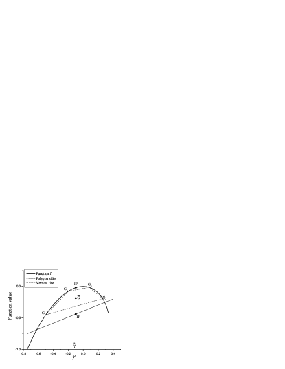
Figure 2: The graphical representation the maximization procedure for the two-photon subspace. The set of points $G_{j}$ corresponds to the output ensemble. The difference $f(\gamma)-g(\gamma)$ over $\gamma$ needs to be maximized over the interval $[\alpha,\beta]$.

IV.3 Graphical interpretation

The result of Lemma 2 can be visualized using the following geometrical reasoning depicted in Fig. 2. Consider a graph of the function $f(\gamma)$ versus its argument $\gamma$. The numbers $\gamma_{j}$ and the corresponding values of the function $f$ are given by a set of points $G_{j}=(\gamma_{j},f(\gamma_{j}))$ in the plane of the graph. The probability distribution $q_{j}$ for the arguments $\gamma_{j}$ defines an average

$$\bar{G}=\left(\sum_{j}q_{j}\gamma_{j},\sum_{j}q_{j}f(\gamma_{j})\right)$$ (33)

that can be interpreted as a center of gravity for the system of points $G_{j}$ that have been assigned respective masses $q_{j}$. Obviously, if the probability distribution is arbitrary, then this average can lie anywhere within the convex polygon spanned by the points $G_{j}$. Since the function $f$ is strictly concave over the range considered, the whole polygon lies within the area bounded by the graph of the function $f(\gamma)$ on one side, and a straight line connecting the points $(\alpha,f(\alpha))$ and $(\beta,f(\beta))$ on the other side. This straight line is given by a function $g$ defined as:

$$g(\gamma)=\frac{\beta-\gamma}{\beta-\alpha}f(\alpha)+\frac{\gamma-\alpha}{\beta-\alpha}f(\beta).$$ (34)

The left hand side of Eq. (27) is now given by the length of a vertical line connecting $\bar{G}$ with the point $H^{\prime}=(\bar{\gamma},f(\bar{\gamma}))$ on the graph of the function $f(\gamma)$, where $\bar{\gamma}=\sum_{j}q_{j}\gamma_{j}$. Clearly, the line $\bar{G}H^{\prime}$ will be always equal in length or shorter than the line $H^{\prime}H^{\prime\prime}$ where the point $H^{\prime\prime}=(\bar{\gamma},g(\bar{\gamma}))$ lies on the graph of the function $g(\gamma)$. Furthermore, in order to find the maximum possible length of the line $H^{\prime}H^{\prime\prime}$, it is clear from this geometric construction that we need to maximize the difference $f(\gamma)-g(\gamma)$ over $\gamma$ belonging to the interval $[\alpha,\beta]$. This procedure is expressed explicitly in the right hand side of Eq. (27) and the parameter $\mu$ introduced in the previous subsection is simply the gradient of the function $g(\gamma)$.

It is clearly seen from this geometric construction that enlarging the interval $[\alpha,\beta]$ can only increase the value of the upper bound given in Eq. (27). This implies two rather straightforward observations. First, the use of entangled states should give a larger capacity compared to separable states. Secondly, a lower value of the parameter $\eta$ meaning weaker correlations between consecutive polarization rotations results in a decreased channel capacity.

The graphical construction presented above also gives a simple recipe for constructing an output ensemble that saturates the bound on the Holevo quantity. It is sufficient to take a two-element ensemble with the extreme points of the allowed interval as the parameters of the Werner states emerging from the channel: $\alpha=\eta c_{\text{min}}$ and $\beta=\eta c_{\text{max}}$. The optimal probabilities of using the two states need to be selected in such a way that the weighted sum of the points corresponding to these states gives the point $\gamma_{\text{opt}}$ maximizing the difference $f(\gamma)-g(\gamma)$. Explicitly, these probabilities are respectively given by $(\beta-\gamma_{\text{opt}})/(\beta-\alpha)$ and $(\gamma_{\text{opt}}-\alpha)/(\beta-\alpha)$. The actual graph of the function $f(\gamma)$ with the permitted ranges of the Werner parameter for perfectly correlated noise and entangled and separable inputs is shown in Fig. 3.

Figure 3: Depiction of the optimal ensembles that maximize the Holevo quantity in both the general entangled case and the restricted separable case, for perfectly correlated noise ($\eta=1$). It is sufficient to take only two-element ensembles with the extreme points of the allowed interval. For general entangled states the interval is $[-1,1/3]$ whereas for the separable case the interval is reduced to $[-1/3,1/3]$

V Attainability and implementation

The Holevo quantity $\chi$ is only an upper bound on the channel capacity and therefore is not necessarily attainable. Users of a communication channel need two relevant pieces of information. The first one is the optimal form of the input ensemble that should be used by the sender. The second one is a measurement scheme that should be employed at the output of the channel in order to optimize the capacity.

Let us start by summarizing the results of the preceding section and specifying the input ensemble implied by these considerations. We have seen that in the zero- and one-photon subspaces the channel capacity cannot be enhanced by exploiting the polarization degree of freedom. Therefore as the elements of the input ensemble we can take for example states $|0_{A}0_{B}\rangle$, $|\updownarrow_{A}0_{B}\rangle$, and $|0_{A}\updownarrow_{B}\rangle$, where for concreteness we have fixed the polarization of single-photon states to vertical. The polarization degree of freedom starts to play a nontrivial role when both the temporal slots are occupied by photons. In this subspace, we need to select two input states characterized by the Werner parameters that are as distant as it is allowed by the constraints on the input ensemble. If we restrict ourselves to separable states, then according to Eq. (23) we need to take one separable state with $c_{\text{min}}=-1/3$ and another one with $c_{\text{max}}=1/3$. It is easy to verify using Eq. (20) that the pair of separable states satisfying this condition can be taken as $|\updownarrow_{A}\leftrightarrow_{B}\rangle$ and $|\updownarrow_{A}\updownarrow_{B}\rangle$. We thus see that in agreement with the simple picture developed in the introduction to this paper, the relevant quantity is the relative polarization of the photons occupying consecutive slots. If we allow for entangled input, then the lower limit for the Werner parameters of the input states shifts down to $c_{\text{min}}=-1$. This value can be of course attained by taking the singlet state $|\Psi_{-}\rangle$ itself as one element of the input ensemble, and any state with $c_{\text{max}}=1/3$, for example again $|\updownarrow_{A}\updownarrow_{B}\rangle$ as the second one.

In order to complete the description of the communication protocol, we need to specify the measurement applied to the states emerging from the channel. This task can be decomposed into two steps. The first one is the determination of the total number of photons contained in the two slots and it can in principle be accomplished by a collective quantum non-demolition measurement QND on all the modes involved that would determine the total photon number without destroying coherence between the modes. Depending on the outcome, the second step needs to be either finding the temporal slot occupied by a photon in the one-photon subspace which can be realized by direct temporally resolved detection, or discriminating between the states used to encode information in the two-photon subspace. It is easy to see that this discrimination takes a simple form in the case of perfectly correlated noise and entangled input states: we need to determine whether the received states belong to the singlet or the triplet subspace, which corresponds to a two-element projective measurement:

$$\hat{\cal{O}}_{S} = |\Psi_{-}\rangle\langle\Psi_{-}|$$

$$\hat{\cal{O}}_{T} = \hat{\openone}-|\Psi_{-}\rangle\langle\Psi_{-}|$$ (35)

It turns out that the same measurement saturates the Holevo bound also in the general case of any value of the parameter $\eta$ with either entangled or separable input states. In Fig. 4(a) we depict conditional probabilities of obtaining the singlet or the triplet outcomes for a two-element input ensemble characterized by Werner parameters $c_{\text{min}}$ and $c_{\text{max}}$. A lengthy but straightforward calculation shows that if we take as the input probabilities the values discussed in the preceding section, the mutual information is given exactly by the right hand side of Eq. (31). Thus the described procedure indeed maximizes the channel capacity in the two-photon subspace.

Figure 4: Depiction of the outcomes of operator measurements $\hat{\cal O}_{S}$ and $\hat{\cal O}_{T}$. The general case is shown in (a). For perfectly correlated noise, when the full range of allowed entangled states is employed, perfect distinguishability between the two inputs is possible as shown in (b). In the restricted separable states only regime, the diagram reduces to that shown in (c) and the emerging states are unable to be distinguished unambiguously.

It is instructive to compare the above diagram for optimal entangled and separable input ensembles in the case of perfect correlations $\eta=1$. For the optimal entangled ensemble, shown in Fig. 4(b) we can distinguish perfectly between the two inputs as they belong to orthogonal subspaces even after the transmission. For the separable ensemble, the emerging states can no longer be perfectly discriminated as seen in Fig. 4(c).

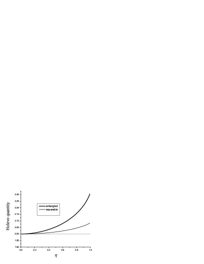
Figure 5: Graph showing plot of $\chi$ versus $\eta$. The channel capacity for the general case where entangled states are used is significantly greater than for the restricted case where only separable states are employed. The dashed line is the channel capacity when the polarization degree of freedom is not used at all.

The complete channel capacity obtained by combining Eq. (8) with the results of Sec. IV is shown as a function of $\eta$ in Fig. 5. It is seen that using an entangled input ensemble gives a clear advantage over the separable states over the complete range of the correlation parameter $\eta$.

We note that the measurement discriminating between the singlet and the triplet subspaces can be implemented using the Braunstein-Mann scheme based on linear optics BrauMannPRA95 , as we do not have to distinguish between all four Bell states. After overlapping temporally the received photons and interfering them on a 50:50 non-polarizing beam splitter, their detection in the same output port corresponds to a projection onto the triplet subspace, whereas measuring them in the separate output ports of the beam splitter identifies the singlet state.

VI Conclusions

We have introduced a model of a communication channel with correlated noise motivated by random birefringence fluctuations in a fiber optic link. Within this model, we have demonstrated that introducing quantum correlations between consecutive uses of the channel increases its capacity. This demonstrates how specifically quantum phenomena such as entanglement can be helpful in the task of transferring classical information. Making use of entanglement requires more complex preparation procedures that provide joint input states extending over a number of temporal slots. A related question is the role of collective quantum measurements on the output of the channel rather than detecting radiation in each of the slots individually and combining classical outcomes of separate measurements.

The action of the channel has been defined in terms of transformations of the bosonic field operators. This opens up a route towards interesting generalizations of the present work, for example including arbitrary multiphoton states. Another direction would be extending the model to an arbitrary number of temporal slots rather than just allowing for correlations between pairs of consecutive slots as in our example. It is easy to give a simple protocol showing that in this case the channel capacity can be enhanced even further. Suppose that the sender generates a train of zero- and one-photon states with the same probabilities equal to one half. The first time she is to transmit a photon, she sends half of maximally entangled pair. In the second instance when a one photon should be transmitted, she sends the remaining member of the pair transforming it in such a way that the joint two-photon polarization state belongs either to the singlet or the triplet subspace. The receiver implements a polarization-independent quantum non-demolition measurement on each temporal slot. When a photon is detected, it needs to be stored until the arrival of the second member of a pair, when the discrimination between the singlet and the triplet subspaces can be performed with the help of a joint measurement. If the fluctuations in random birefringence can be neglected over the temporal separation between the photons in a pair, this procedure allows one to encode one extra bit of information into each pair of transmitted photons. This gives the average channel capacity equal to $2.5$ per a pair of temporal slots, enhancing further the optimal value shown in Fig. 5.

References

- (1) M. A. Nielsen and I. L. Chuang, Quantum Computation and Quantum Information (Cambridge University Press, Cambridge, 2000).
- (2) A. Ghatak and K. Thyagarajan, Introduction to Fiber Optics (Cambridge University Press, Cambridge, 1998).
- (3) E. Kashefi, A. Kent, V. Vedral, and K. Banaszek, Phys. Rev. A 65, 050304(R) (2002).
- (4) C. Macchiavello, G. M. Palma, Phys. Rev A 65, 050301 (2002).
- (5) C. H. Bennett, P. W. Shor, J. A. Smolin, and A. V. Thapliyal, Phys. Rev. Lett. 83, 3081 (1999).
- (6) Z. D. Walton, A. F. Abouraddy, A. V. Sergienko, B. E. A. Saleh, and M. C. Teich, Phys. Rev. Lett. 91, 087901 (2003).
- (7) J.-C. Boileau, D. Gottesman, R. Laflamme, D. Poulin, and R. W. Spekkens, quant-ph/0306199.
- (8) P. Hausladen, R. Jozsa, B. Schumacher, M. Westmoreland, and W. K. Wootters, Phys. Rev. A 54, 1869 (1996).
- (9) A. S. Holevo, Prob. Inf. Transm. 5, 247 (1979).
- (10) R. A. Campos, B. E. A. Saleh, and M. C. Teich, Phys. Rev. A 40, 1371 (1989).
- (11) M. Born and E. Wolf, Principles of Optics, 7th Ed. (Cambridge University Press, Cambridge, 1999).
- (12) D. M. Brink and G. R. Satchler, Angular Momentum, 2nd Ed. (Clarendon, Oxford, 1968).
- (13) R. F. Werner, Phys. Rev. A 40, 4277 (1989).
- (14) R. Horodecki and M. Horodecki, Phys. Rev. A 54, 1838 (1996).
- (15) P. Grangier, J. A. Levenson, and J.-P. Poizat, Nature 396, 537 (1998).
- (16) S. L. Braunstein and A. Mann, Phys. Rev. A 51, R1727 (1995)