On improving single photon sources via linear optics and photodetection

Abstract

In practice, single photons are generated as a mixture of vacuum with a single photon with weights $1-p$ and $p$, respectively; here we are concerned with increasing $p$ by directing multiple copies of the single photon-vacuum mixture into a linear optic device and applying photodetection on some outputs to conditionally prepare single photon states with larger $p$. We prove that it is impossible, under certain conditions, to increase $p$ via linear optics and conditional preparation based on photodetection, and we also establish a class of photodetection events for which $p$ can be improved. In addition we prove that it is not possible to obtain perfect ($p=1$) single photon states via this method from imperfect ($p<1$) inputs.

Single photon sources are important, for example to achieve secure quantum key distribution key and for linear optic quantum computation LOQC , yet generating single photons remains challenging. The traditional method involves photodetection on one output mode from a nondegenerate parametric downconversion process to post-select a single photon in the correlated mode down . More recently alternative single-photon sources have been employed, including molecules mol , quantum wells well , color centers col , ions ion and quantum dots dot . In these examples, the probability of more than one photon being produced is much lower than that for a Poissonian process, but the vacuum contribution can be quite high. Under ideal conditions, with a single mode output stable over time, the output state can be described by the density matrix

$$\hat{\rho}_{p}=(1-p)|{0}\rangle\langle{0}|+p|{1}\rangle\langle{1}|,$$ (1)

with $p$ the probability of obtaining a single photon; $p$ is sometimes referred to as the efficiency for producing single photons. Whereas the theoretical single-photon state corresponds to $p=1$, the experimental single-photon state is a mixture of the single photon with the vacuum.

Increasing the value of $p$ (the efficiency of producing single photons) is an increasingly important objective because of requirements for quantum optics experiments, especially those concerned with quantum information processing. Much of this effort is directed to improving sources, but here we pose the question as to whether a source of single photons with efficiency $p$ can be processed via linear optics and photodetection to yield fewer photons but with higher $p$. More specifically, would it be possible to direct $N$ copies of these single photon states with efficiency $p$ into an $N$-channel passive interferometer (an interferometer that involves only passive, linear optical elements) to yield an output single photon with efficiency $p^{\prime}>p$ for certain photodetection records on the other outputs? If the answer is yes, then interferometry and photodetection could be employed to improve the efficiency of single-photon sources.

In fact the answer will be no, provided we consider detection results where all but one of the photons are detected. This is the most straightforward way of ensuring that the output state contains at most one photon. This restriction is necessary in most applications of linear optics quantum information processing since two-photon contributions can have unwanted side effects, e.g. allowing for certain multiphoton attacks in quantum key distribution applications. If we allow other detection results, it is possible for low-efficiency (small $p$) single-photon states to yield, via linear optics and conditional preparation based on photodetection, an output with a larger probability for a single photon. However, these schemes also yield non-zero probabilities for photon numbers above one.

A passive interferometer is comprised of beam splitters, mirrors, and phase shifters. Each of these elements preserves total photon number from input to output under ideal conditions. No energy is required to operate these optical elements, hence the term passive. These are also known as linear optical elements. More generally polarization transforming elements can be included, but here we are concerned only with a scalar field treatment; in fact polarization effects could be included by doubling the number of channels and treating the two polarizations in a mode as two separate channels. Mathematically, a passive interferometer transforms the amplitude operators of the incoming fields $\hat{\bm{a}}$ via the matrix transformation $\hat{\bm{a}}^{\dagger}\mapsto\bm{\Lambda}^{T}\hat{\bm{a}}^{\dagger}$ with $\Lambda\in\text{U}(N)$ VogelWelsch .

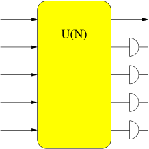
Figure 1: Schematic setup of the network. We assume $N$ incoming modes prepared in the state (On improving single photon sources via linear optics and photodetection) with different $p_{i}$.

In the general case we start with a supply of $N$ mixed states of the form (1). For additional generality we allow the different inputs to have different probabilities for finding a single photon, $p_{i}$, and we denote the maximum of these probabilities by $p_{\rm max}$. The initial state may be expressed as

$$\hat{\rho}_{\text{in}}^{(N)} =\bigotimes_{i=1}^{N}\big{[}(1-p_{i})|{0}\rangle\langle{0}|+p_{i}|{1}\rangle\langle{1}|\big{]}$$

$$=\sum_{\bm{s}}P_{\bm{s}}\left(\prod_{i}(\hat{a}_{i}^{\dagger})^{s_{i}}|{0}\rangle\otimes\text{h.c.}\right),$$ (2)

where $P_{\bm{s}}$ $\!=$ $\!\prod_{i}p_{i}^{s_{i}}(1-p_{i})^{1-s_{i}}$, and the vector $\bm{s}$ $\!=$ $\!(s_{1},\cdots,s_{N})^{T}$, ($s_{i}=0,1$), gives the photon numbers in the inputs. The interferometer transformation $\hat{\bm{a}}^{\dagger}\mapsto\bm{\Lambda}^{T}\hat{\bm{a}}^{\dagger}$ results in the output state

$$\hat{\rho}_{\rm trans}^{(N)}=\sum_{\bm{s}}P_{\bm{s}}\left[\prod_{i}\left(\sum_{k}\Lambda_{ki}\hat{a}_{k}^{\dagger}\right)^{s_{i}}|{0}\rangle\otimes\text{h.c.}\right].$$ (3)

Without loss of generality, we take mode 1 to be the mode in which we wish to improve the photon statistics. We perform photodetections on the other $N-1$ modes, and examine the final state in mode 1 conditioned on the results of these photodetections. The total number of photons detected is $D$, and the number of photons detected in mode $j$ is $n_{j}$ (see Fig. 1). It is easy to see that no better result can be obtained by performing photodetections on fewer than $N-1$ modes; this would be equivalent to averaging over the photocounts for some of the modes. We assume ideal photodetection in this analysis in order to determine the best results possible using linear optics and photodetection.

The conditional state in mode 1 after photodetection in modes 2 to $N$ is

$$\hat{\rho}_{\rm out}^{(N)}=\sum_{n_{1}=0}^{N}c_{n_{1}}|{n_{1}}\rangle\langle{n_{1}}|,$$ (4)

where $n_{1}$ is the photon number in the remaining output mode (rather than the number of photons detected at a photodetector). Each coefficient $c_{n_{1}}$ is given by

$$c_{n_{1}}=K\langle{\bm{n}}|\hat{\rho}_{\rm trans}^{(N)}|{\bm{n}}\rangle,$$ (5)

where $|{\bm{n}}\rangle$ is a tensor product of number states in each of the output modes. The normalization constant $K$ equals

$$K=\left[\sum_{n_{1}=0}^{N}\langle{\bm{n}}|\hat{\rho}_{\rm trans}^{(N)}|{\bm{n}}\rangle\right]^{-1}.$$ (6)

In order to find the expectation value in Eq. (5), we first introduce some notation. Let $\Phi_{\bm{s}}=\{i|s_{i}=1\}$, $\Sigma_{\bm{s}}=\sum_{i}s_{i}$ (so $\Sigma_{\bm{s}}$ is the number of elements in $\Phi_{\bm{s}}$), and let ${\rm Y}_{\bm{s}}$ be the set that consists of all vectors comprised of the elements of $\Phi_{\bm{s}}$. In addition we use the notation $K^{\prime}=K/\prod_{j=2}^{N}n_{j}!$ and $\Sigma_{\bm{n}}=\sum_{j}n_{j}$. Using this notation, $c_{1}$ is given by

$$c_{1}=\frac{K^{\prime}}{n_{1}!}\sum_{\bm{s};\Sigma_{\bm{s}}=\Sigma_{\bm{n}}}P_{\bm{s}}\left|S_{\bm{s},\bm{n}}\right|^{2},$$ (7)

where

$$S_{\bm{s},\bm{n}} =\sum_{\bm{\sigma}\in{\rm Y}_{\bm{s}}}\left(\Lambda_{1,\sigma_{1}}\cdots\Lambda_{1,\sigma_{n_{1}}}\right)$$

$$\cdots\left(\Lambda_{N,\sigma_{\Sigma_{\bm{n}}-n_{N}+1}}\cdots\Lambda_{N,\sigma_{\Sigma_{\bm{n}}}}\right).$$ (8)

In order to determine if there is an improvement in the probability of finding a single photon, we need to determine the value of $c_{1}$. However, determining $c_{1}$ requires evaluating $K$, which requires evaluating the expectation values in Eq. (5) for all possible values of $n_{1}$. Instead, we will consider the ratio $c_{1}/c_{0}$. There are three main advantages to considering this quantity:
1. The common constant $K^{\prime}$ cancels, so this expression is easily evaluated analytically.
2. If $c_{1}/c_{0}$ is not greater than $R\equiv p_{\rm max}/(1-p_{\rm max})$, then it is clear that $c_{1}\leq p_{\rm max}$. Thus we can determine those cases where there is no improvement.
3. For $p_{\rm max}\ll 1$, $c_{0}\approx 1$ and $R\approx p_{\rm max}$. Therefore the improvement in $c_{1}/c_{0}$ over $R$ is approximately the same as the improvement in the probability of a single photon over $p_{\rm max}$.

Ideally, we would determine the interferometer and detection pattern such that $c_{1}/c_{0}$ is maximized, but this does not appear to be possible analytically. However, we can place an upper limit on $c_{1}/c_{0}$ in the following way. Let us express the summation for $c_{0}$ as

$$c_{0}=\frac{K^{\prime}}{N-D}\sum_{\bm{s};\Sigma_{\bm{s}}=D+1}\sum_{k;s_{k}=1}P_{\bm{s}^{k}}\left|S_{\bm{s}^{k},\bm{n}^{\prime}}\right|^{2},$$ (9)

where $s^{k}_{i}=s_{i}$ except for $s^{k}_{k}=0$, and $n^{\prime}_{j}=n_{j}$ except $n^{\prime}_{1}=0$. The quotient of $N-D$ takes account of a redundancy in the sum. Each alternative input $\bm{s}^{k}$ has $N-D$ zeros, so there are $N-D$ possible alternative $\bm{s}$ that give the same $\bm{s}^{k}$. We may reduce this quotient slightly if we take account of the possibility that some of the inputs have zero photon probability. Let there be $N-M$ inputs with $p_{i}=0$, so the maximum total number of photons is $M$. If we limit the first sum in Eq. (9) to $\bm{s}$ such that $P_{\bm{s}}\neq 0$, then the redundancy is $M-D$. Therefore we obtain

$$c_{0} =\frac{K^{\prime}}{M-D}\sum_{\begin{subarray}{c}\bm{s};P_{\bm{s}}\neq 0\\ \Sigma_{\bm{s}}=D+1\end{subarray}}\sum_{k;s_{k}=1}P_{\bm{s}^{k}}\left|S_{k}\right|^{2}$$

$$=\frac{K^{\prime}}{M-D}\sum_{\begin{subarray}{c}\bm{s};P_{\bm{s}}\neq 0\\ \Sigma_{\bm{s}}=D+1\end{subarray}}P_{\bm{s}}\sum_{k;s_{k}=1}\frac{1-p_{k}}{p_{k}}\left|S_{k}\right|^{2},$$ (10)

where $S_{k}=S_{\bm{s}^{k},\bm{n}^{\prime}}$. Since we have limited the sum to terms where $P_{\bm{s}}\neq 0$, $p_{k}$ is nonzero, and thus the ratio $(1-p_{k})/p_{k}$ does not diverge. Since $p_{k}$ does not exceed $p_{\rm max}$, we have the inequality

$$c_{0}\geq\frac{K^{\prime}}{M-D}\frac{1-p_{\rm max}}{p_{\rm max}}\sum_{\bm{s};\Sigma_{\bm{s}}=D+1}P_{\bm{s}}\sum_{k;s_{k}=1}\left|S_{k}\right|^{2}.$$ (11)

Here we are able to omit the condition $P_{\bm{s}}\neq 0$ because terms with $P_{\bm{s}}=0$ are zero anyway. We may re-express the equation for $c_{1}$ as

$$c_{1}=K^{\prime}\sum_{\bm{s};\Sigma_{\bm{s}}=D+1}P_{\bm{s}}\left|\sum_{k;s_{k}=1}\Lambda_{1k}S_{k}\right|^{2}.$$ (12)

We therefore obtain

$$c_{1}\leq K^{\prime}\sum_{\bm{s};\Sigma_{\bm{s}}=D+1}P_{\bm{s}}\sum_{k;s_{k}=1}\left|S_{k}\right|^{2}.$$ (13)

Combining Eqs. (11) and (13) gives

$$\frac{c_{1}}{c_{0}}\leq(M-D)\frac{p_{\rm max}}{1-p_{\rm max}}.$$ (14)

This yields an upper limit on the ratio between the one and zero photon probabilities. One application of this result is that it is impossible to get one photon with unit probability, as it would be necessary for this ratio is infinite. Another consequence of (14) is that for $D=M-1$ (i.e. the number of photons detected one less the maximum input number) an improvement can never be achieved. This case is important because it is the most straightforward way of eliminating the possibility of two or more photons in the output mode.

In the remainder of this article, we will investigate situations in which the single-photon contribution can be enhanced. As $M\leq N$, and $D\geq 0$, the upper limit on the improvement in $c_{1}/c_{0}$ is simply $N$. This is also the upper limit in how far $c_{1}$ can be increased above $p_{\rm max}$. We will now consider a scheme that gives a linear improvement in $c_{1}/c_{0}$, though not as high as $N$. In order to obtain a large value for the ratio $c_{1}/c_{0}$, we want the inequality in Eq. (13) to be as close to equality as possible. In turn, this means that we want the vectors $(\Lambda_{1k})$ and $(S_{k})$ to be as close to parallel as possible. For this, we consider the interferometer given by

$$\Lambda_{21}=-\epsilon, \quad\Lambda_{22}=\sqrt{1-\epsilon},$$

$$\Lambda_{i1}=\sqrt{(1-\epsilon^{2})/(N-1)}, \quad\Lambda_{i2}=\epsilon/\sqrt{N-1},$$ (15)

for $i\neq 2$ (the values of $\Lambda_{ij}$ for $j>2$ do not enter into the analysis). Here $\epsilon$ is a small number, and we will ignore terms of order $\epsilon$ or higher. Now let $p_{i}=p_{\rm max}$, and consider the measurement record where zero photons are detected in modes 3 to $N$, and $D$ photons are detected in output mode 2. To determine $c_{n_{1}}$, note first that $\Lambda_{22}\gg\Lambda_{2i}$ for $i\neq 2$, so we may ignore those terms in the sum for $S_{\bm{s},\bm{n}}$ where $\Lambda_{22}$ does not appear. Each term has magnitude $\Lambda_{11}^{n_{1}}\Lambda_{22}\Lambda_{21}^{D-1}$ , and there are $D(D+n_{1}-1)!$ such terms. Therefore, provided $s_{2}=1$,

$$S_{\bm{s},\bm{n}}\approx D(D+n_{1}-1)!\Lambda_{11}^{n_{1}}\Lambda_{22}\Lambda_{21}^{D-1}\,,\quad\epsilon\ll 1.$$ (16)

In the summation for $c_{n_{1}}$, we have $\binom{N-1}{D-n_{1}-1}$ different combinations of inputs such that $\Sigma_{\bm{s}}=D+n_{1}$ and $s_{2}=1$. Combining these results, we have

$$c_{n_{1}} \approx\frac{K^{\prime}}{n_{1}!}p_{\rm max}^{D+s_{1}}(1-p_{\rm max})^{N-D-s_{1}}$$

$$\times\frac{(N-1)!D^{2}(D+n_{1}-1)!}{(N-D-n_{1})!}\Lambda_{11}^{2n_{1}}\Lambda_{22}^{2}\Lambda_{21}^{2D-2}$$

$$\approx K^{\prime\prime}\left(\frac{R}{N-1}\right)^{n_{1}}\frac{(D+n_{1}-1)!}{n_{1}!(N-D-n_{1})!},$$ (17)

We have combined those factors that do not depend on $n_{1}$ into a new constant $K^{\prime\prime}$, and used $\Lambda_{11}\approx 1/\sqrt{N-1}$.

Using Eq. (On improving single photon sources via linear optics and photodetection) we find that

$$\frac{c_{1}}{c_{0}}\approx R\frac{D(N-D)}{N-1}\,,\quad\epsilon\ll 1.$$ (18)

The maximum improvement in the ratio $c_{1}/c_{0}$ is obtained for $D=\lceil N/2\rceil$, where $c_{1}/c_{0}=R\lfloor N^{2}/4\rfloor/(N-1)$. The multiplying factor $\lfloor N^{2}/4\rfloor/(N-1)$ is larger than 1 for all $N\geq 4$. Thus we find that, provided there are at least 4 modes, we may obtain an improvement in the ratio $c_{1}/c_{0}$. For $p_{\rm max}\ll 1$, $c_{1}\approx p_{\rm max}\lfloor N^{2}/4\rfloor/(N-1)$. For large $N$, the probability of a single photon increases approximately as $N/4$. This is linear with $N$, but is not quite as large as the upper limit of $N$.

However, there are some drawbacks to this interferometry scheme [i.e. using the interferometer (On improving single photon sources via linear optics and photodetection)]. The first drawback is the two-photon contribution. We find that

$$\frac{c_{2}/c_{1}}{c_{1}/c_{0}}=\frac{(D+1)(N-D-1)}{2D(N-D)}\,,$$ (19)

which, for $D=\lceil N/2\rceil$, is less than $1/2$, but it is close to $1/2$ for large $N$. Since this is the same ratio as for a Poisson distribution, this is equivalent to using a coherent state. The two-photon contribution can be reduced by using larger $D$, but this is at the expense of reducing $c_{1}$.

The second drawback is that improvements are only obtained for small $p_{\rm max}$. Although the improvement in the ratio $c_{1}/c_{0}$ is independent of $p_{\rm max}$, improvements in $c_{1}$ can only be obtained for values of $p_{\rm max}$ below $1/2$. That is, this method can only be used to obtain improvements in the probability of a single photon up to $1/2$, but not to make the probability of a single photon arbitrarily close to 1. Note that the above method only gives $c_{1}>p_{\rm max}$ for four or more modes. We will now show that it is impossible to obtain an improvement in the probability of a single photon with fewer than four modes, and for various combinations of detections with larger numbers of modes.

We first examine the case $D=0$. Then we have only one term in the sum for $c_{0}$, and $c_{0}=K^{\prime}P_{\bm{0}}$. The expression for $c_{1}$ becomes

$$c_{1} =K^{\prime}\sum_{k=1}^{N}\frac{p_{k}}{1-p_{k}}P_{\bm{0}}\left|\Lambda_{1k}\right|^{2}\leq K^{\prime}\frac{p_{\rm max}}{1-p_{\rm max}}\sum_{k=1}^{N}P_{\bm{0}}\left|\Lambda_{1k}\right|^{2}$$

$$=K^{\prime}RP_{\bm{0}}=c_{0}R.$$ (20)

Thus we have shown that $c_{1}/c_{0}\leq R$, so $c_{1}\leq p_{\rm max}$. Hence there can be no improvement in the photon statistics if zero photons are detected. We can also obtain a similar result for the case $D=1$, provided all the input $p_{i}$ are equal. In that case, we have

$$c_{0}=K^{\prime}\sum_{k}\frac{p_{\rm max}}{1-p_{\rm max}}P_{\bm{0}}\left|\Lambda_{2k}\right|^{2}=K^{\prime}RP_{\bm{0}}.$$ (21)

The value of $c_{1}$ is given by

$$c_{1} =\frac{1}{2}K^{\prime}\sum_{k}\sum_{l;l\neq k}R^{2}P_{\bm{0}}\left|\Lambda_{1l}\Lambda_{2k}+\Lambda_{1k}\Lambda_{2l}\right|^{2}$$

$$\leq\frac{1}{2}K^{\prime}R^{2}P_{\bm{0}}\sum_{k,l}\left|\Lambda_{1l}\Lambda_{2k}+\Lambda_{1k}\Lambda_{2l}\right|^{2}=K^{\prime}R^{2}P_{\bm{0}}.$$ (22)

In the last line we have used the fact that $\Lambda_{1k}$ and $\Lambda_{2k}$ are orthonormal. Thus we again find $c_{1}/c_{0}\leq R$, so $c_{1}\leq p_{\rm max}$.

These results clearly eliminate the possibility of improving the probability of finding one photon with a two-mode interferometer. We have shown that detecting zero photons does not give an improvement, and if one photon is detected, then we must have $M-D=1$ or 0, so there again can be no improvement. Along the same lines we can also eliminate the three-mode interferometer.

We have shown that it is impossible to improve the efficiency of a single-photon source by channeling more than one low-efficiency single-photon state into a linear optic interferometer and detecting all but one of the photons. This eliminates the most straightforward scheme for obtaining an output state with no more than one photon. It is possible to obtain an improvement for more general detection results, but at the expense of non-zero probabilities for two or more photons. We have not proven that it is impossible to obtain an improvement in the probability of a single photon while restricting to zero probability for two or more photons; however, numerical searches indicate that it is unlikely.

This work was funded in parts by the UK Engineering and Physical Sciences Research Council. One of the authors (SS) enjoys a Feodor-Lynen fellowship of the Alexander von Humboldt foundation. BCS appreciates valuable discussions with R. Laflamme in the early stages of this work. This research has also been supported by an Australian Department of Education Science and Training Innovation Access Program Grant to support collaboration in the European Fifth Framework project QUPRODIS, and by Alberta’s informatics Circle of Research Excellence (iCORE).

References

• (1) G. Brassard, N. Lรผtkenhaus, T. Mor, and B. Sanders, Phys.ย Rev.ย Lett.ย 85, 1330 (2000); G. Brassard and C. Crรฉpeau, SIGACT News 27, 13 (1996).
• (2) E. Knill, R. Laflamme, and G.J. Milburn, Nature 409, 46 (2001); S. Scheel, K. Nemoto, W.J. Munro, and P.L. Knight, Phys.ย Rev.ย A(accepted June 2003).
• (3) C. K. Hong and L. Mandel, Phys.ย Rev.ย Lett.ย 56, 58 (1986).
• (4) F. DeMartini, G. DiGuiseppe, and M. Marrocco, Phys.ย Rev.ย Lett.ย 76, 900 (1996); C. Brunel, B. Lounis, P. Tamarat, and M. Orrit, Phys.ย Rev.ย Lett.ย 83, 2722 (1999); B. Lounis and W.E. Moerner, Nature 407, 491 (2000).
• (5) J. Kim, O. Benson, H. Kan, and Y. Yamamoto, Nature 397, 500 (1999);
• (6) C. Kurtsiefer, S. Mayer, P. Zarda, and H. Weinfurter, Phys.ย Rev.ย Lett.ย 85, 290 (2000); R. Brouri, A. Beveratos, J.P. Poizat, and P. Grangier, Opt. Lett. 25, 1294 (2000); A. Beveratos et al., Eur. Phys. J. D 18, 191 (2002).
• (7) A. Kuhn, M. Hennrich, T. Bondo, and G. Rempe, Appl. Phys. B 69, 373 (1999); B.T.H. Varcoe, S. Brattke, M. Weidinger, and H. Walther, Nature 403, 743 (2000); A. Kuhn, M. Hennrich, and G. Rempe, Phys.ย Rev.ย Lett.ย 89, 067901 (2002).
• (8) P. Michler et al., Science 290, 2282 (2000); C. Santori, M. Pelton, G. Solomon, Y. Dale, and Y. Yamamoto, Phys.ย Rev.ย Lett.ย 86, 1502 (2001); V. Zwiller et al., Appl. Phys. Lett. 78, 2476 (2001); E. Moreau et al., Appl. Phys. Lett. 79, 2865 (2001); Z. Yuan et al. Science 295, 102 (2002); J.-M. Gรฉrard and B. Gayral, J. Lightwave Technol. 17, 2089 (1999); C. Santori et al., Nature 419, 594 (2002).
• (9) W. Vogel, S. Wallentowitz, and D.-G. Welsch, Quantum Optics: An Introduction (Wiley-VCH, Berlin, 2001).
• (10) L. Knรถll, S. Scheel, E. Schmidt, D.-G. Welsch, and A.V. Chizhov, Phys. Rev. A 59, 4716 (1999).