Comparison of Theory and Experiment
for a One-Atom Laser in a Regime of Strong Coupling

Abstract

Our recent paper reports the experimental realization of a one-atom laser in a regime of strong coupling mckeever03b . Here we provide the supporting theoretical analysis relevant to the operating regime of our experiment. By way of a simplified four-state model, we investigate the passage from the domain of conventional laser theory into the regime of strong coupling for a single intracavity atom pumped by coherent external fields. The four-state model is also employed to exhibit the vacuum-Rabi splitting and to calculate the optical spectrum. We next extend this model to incorporate the relevant Zeeman hyperfine states as well as a simple description of the pumping processes in the presence of polarization gradients and atomic motion. This extended model is employed to make quantitative comparisons with the measurements of Ref. mckeever03b for the intracavity photon number versus pump strength and for the photon statistics as expressed by the intensity correlation function $g^{(2)}(\tau)$.

I Introduction

Although a number of theoretical analyses related to a one-atom laser have appeared in the literature mu92 ; ginzel93 ; pellizzari94a ; pellizzari94b ; horak95 ; briegel96 ; meyer97a ; loeffler97 ; meyer97b ; meyer98 ; jones99 ; chough00 ; fidio01 ; kilin02 ; rice03 ; salzburger03 , these prior treatments have not been specific to the parameter range of our recent experiment as reported in Ref. mckeever03b . Because of this circumstance, we have carried out theoretical investigations in support of our experimental program, and present comparisons of these model calculations with our measurements in this paper. In Section II we introduce a simplified four-state model that captures the essential features of the operation of our one-atom laser in a domain of strong coupling but which avoids the complexity of the full Zeeman substructure of the hyperfine levels in atomic Cesium. Sections III and IV then present in turn semiclassical and quantum solutions for this four-state model system. By way of a physically motivated transformation for which the length of a Fabry-Perot cavity is made progressively shorter, we utilize these results to investigate the continuous passage from a domain in which conventional laser theory is applicable into a regime of strong coupling for which the full quantum theory is required. We thereby gain some insight into the relationship of our system to prior theoretical treatments related to the definition of the laser threshold and to “thresholdless” lasing demartini88 ; rice94 ; jin94 ; bjork94 ; protsenko99 . The four-state model is further employed to calculate the intracavity photon number versus pump detuning, thereby exhibiting the “vacuum-Rabi” splitting for the atom-cavity system eberly83 ; agarwal84 ; thompson92 and to compute the optical spectrum of the intracavity field.

In Section V we describe the procedures followed to obtain solutions for an expanded model that incorporates the relevant Zeeman substructure for the Cesium atom ($32$ atomic states), two modes of the cavity with orthogonal polarizations, and a simple model to account for the polarization gradients of the optical fields. Comparisons of the results from quantum jumps simulations based upon this expanded model with our measurements of the mean intracavity photon number $\bar{n}$ versus normalized pump intensity $x$ (Figure 3 of Ref. mckeever03b ) and with our experimental determination of the intensity correlation function $g^{(2)}(\tau)$ (Figure 4 of Ref. mckeever03b ) are given in Sections V(a) and V(b), respectively.

Our intent here is not to belabor the comparison of our experiment with prior work on micro-masers and lasers, for which extensive reviews are available berman94 ; meystre92 ; yamamoto-slusher93 ; chang-campillo96 ; vahala03 . Instead, our principal goal is to establish quantitative correspondence between our measurements and fundamental theoretical models. Having thereby validated the suitability of the theoretical treatments, we can then use these models to inform further experimental investigations of the atom-cavity system.

II Four-state model

We begin with a four-state model to describe our experiment in which a single Cesium atom is trapped inside an optical cavity as illustrated in Figure 1. Although the actual level structure of the Cesium $6S_{1/2}\leftrightarrow 6P_{3/2}$ transition is more complex due to the Zeeman substructure, this simpler model offers considerable insight into the nature of the steady states and dynamics. Following the labelling convention in Fig. 1, we introduce the following set of Hamiltonians $H_{i}$ in a suitably defined interaction picture ($\hslash=1$):

$$\hat{H}_{1} = g_{43}(\hat{a}^{\dagger}\hat{\sigma}_{g4,e3}+\hat{\sigma}_{e3,g4}\hat{a}),$$ (1)

$$\hat{H}_{2} = \frac{1}{2}\Omega_{3}(\hat{\sigma}_{g3,e3}+\hat{\sigma}_{e3,g3}),$$

$$\hat{H}_{3} = \frac{1}{2}\Omega_{4}(\hat{\sigma}_{g3,e3}+\hat{\sigma}_{e3,g3}),$$

$$\hat{H}_{4} = (\Delta_{AC}+\Delta_{4})\hat{a}^{\dagger}\hat{a},$$

$$\hat{H}_{5} = \Delta_{3}\hat{\sigma}_{e3,e3}+\Delta_{4}\hat{\sigma}_{e4,e4},$$

$$\hat{H}_{tot} = \hat{H}_{1}+\hat{H}_{2}+\hat{H}_{3}+\hat{H}_{4}+\hat{H}_{5}\text{ .}$$

In a standard convention, the atomic operators are $\hat{\sigma}_{i,j}\equiv|i\rangle\langle j|$ for states $(i,j)$, with the association of the $F=3,4$ ground and the $F^{\prime}=3^{\prime},4^{\prime}$ levels with $g3,g4,e3,e4$, respectively. The Hamiltonian $\hat{H}_{1}$ accounts for the coherent coupling of the atomic transition $e3\leftrightarrow g4$ to the field of a single mode of the cavity with creation and annihilation operators $(\hat{a}^{\dagger},\hat{a})$. The upper state $e3$ of the lasing transition is pumped by the (coherent-state) field $\Omega_{3}$, while the lower state $g4$ is depleted by the field $\Omega_{4}$ as described by $(\hat{H}_{2},\hat{H}_{3})$, respectively. $(\hat{H}_{4},\hat{H}_{5})$ account for various detunings, including $\Delta_{AC}$ for the offset between the cavity resonance and the $e3\leftrightarrow g4$ atomic transition, $\Delta_{3}$ for the offset between the field $\Omega_{3}$ and the $g3\leftrightarrow e3$ transition, and $\Delta_{4}$ for the offset between the field $\Omega_{4}$ and the $g4\leftrightarrow e4$ transition. Beyond these interactions, we also account for irreversible processes by assuming that the atom is coupled to a continuum of modes other than the privileged cavity mode, and likewise for the coupling of the cavity mode to an independent continuum of external modes.

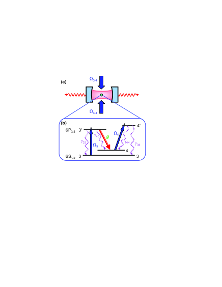
Figure 1: Illustration of a one-atom laser. (a) The atom is located in a high-$Q$ optical cavity of decay rate $\kappa$, and is driven by the fields $\Omega_{3,4}$. (b) Inset of the atomic level scheme relevant to our experiment with the $6S_{1/2}\leftrightarrow 6P_{3/2}$ transition in atomic Cesium. The “lasing” transition is from the excited level $F=3^{\prime}$ to the ground level $F=4$. Pumping of the excited $3^{\prime}$ level is by way of coherent excitation from a laser with Rabi frequency $\Omega_{3}$. Effective decay from the ground $4$ level is provided by the combination of a second field with Rabi frequency $\Omega_{4}$ and spontaneous decay $4^{\prime}\rightarrow 3$. Various radiative decay rates $\gamma_{ij}$ appropriate to the $D_{2}$ line in Cs are given in the text.

With these preliminaries, it is then straightforward to derive a master equation for the density operator $\hat{\rho}$ for the atom-cavity system carmichael-book ; gardiner-book in the Born-Markov approximation. For our model system, this equation is

$$\frac{d\hat{\rho}}{dt}=-i[\hat{H}_{tot},\hat{\rho}]+\sum_{i=1}^{5}\hat{L}_{i},$$ (2)

Here, the terms $\hat{L}_{i}$ account for each of the various decay channels, and are given explicitly by

$$\hat{L}_{1} = \kappa(2\hat{a}\hat{\rho}\hat{a}^{\dagger}-\hat{a}^{\dagger}\hat{a}\hat{\rho}-\hat{\rho}\hat{a}^{\dagger}\hat{a}),$$ (3)

$$\hat{L}_{2} = \gamma_{33}(2\hat{\sigma}_{g3,e3}\hat{\rho}\hat{\sigma}_{e3,g3}-\hat{\sigma}_{e3,e3}\hat{\rho}-\hat{\rho}\hat{\sigma}_{e3,e3}),$$

$$\hat{L}_{3} = \gamma_{43}(2\hat{\sigma}_{g4,e3}\hat{\rho}\hat{\sigma}_{e3,g4}-\hat{\sigma}_{e3,e3}\hat{\rho}-\hat{\rho}\hat{\sigma}_{e3,e3}),$$

$$\hat{L}_{4} = \gamma_{34}(2\hat{\sigma}_{g3,e4}\hat{\rho}\hat{\sigma}_{e4,g3}-\hat{\sigma}_{e4,e4}\hat{\rho}-\hat{\rho}\hat{\sigma}_{e4,e4}),$$

$$\hat{L}_{5} = \gamma_{44}(2\hat{\sigma}_{g4,e4}\hat{\rho}\hat{\sigma}_{e4,g4}-\hat{\sigma}_{e4,e4}\hat{\rho}-\hat{\rho}\hat{\sigma}_{e4,e4})\text{ ,}$$

where the association of each term $\hat{L}_{i}$ with the decay processes in Fig. 1 should be obvious. Spontaneous decay of the various atomic transitions to modes other than the cavity mode proceeds at (amplitude) rate $\gamma_{ij}$ as indicated in Fig. 1, while the cavity (field) decay rate is given by $\kappa$.

The master equation allows us to derive a set of equations for expectation values of atom $\langle\hat{\sigma}_{i,j}\rangle$ and field $\langle\hat{a}\rangle$ operators. One example is for the atomic polarization $\langle\hat{\sigma}_{g4,e3}\rangle$ on the $e3\leftrightarrow g4$ transition, namely

$$\frac{d\langle\hat{\sigma}_{g4,e3}\rangle}{dt} = -\left[(\gamma_{33}+\gamma_{43})+i\Delta_{3}\right]\langle\hat{\sigma}_{g4,e3}\rangle$$

$$-i\left(\Omega_{3}\langle\hat{\sigma}_{g4,g3}\rangle-\Omega_{4}\langle\hat{\sigma}_{e4,e3}\rangle\right)$$

$$+ig_{43}\left(\langle\hat{\sigma}_{e3,e3}\hat{a}\rangle-\langle\hat{\sigma}_{g4,g4}\hat{a}\rangle\right)\text{ .}$$

A solution to this equation requires not only knowledge of single-operator expectation values $\langle\hat{\sigma}_{i,j}\rangle$ and $\langle\hat{a}\rangle$, but also of operator products such as $\langle\hat{\sigma}_{e3,e3}\hat{a}\rangle$. We can develop coupled equations for such products $\langle\hat{\sigma}_{i,j}\hat{a}\rangle$ but would find that their solution requires in turn yet higher order correlations, ultimately leading to an unbounded set of equations.

Conventional theories of the laser proceed beyond this impasse by one of several ultimately equivalent avenues. Within the setting of our current approach, a standard way forward is to factorize operator products in the fashion

$$\langle\hat{\sigma}_{i,j}\hat{a}\rangle=\langle\hat{\sigma}_{i,j}\rangle\langle\hat{a}\rangle+(\langle\hat{\sigma}_{i,j}\hat{a}\rangle-\langle\hat{\sigma}_{i,j}\rangle\langle\hat{a}\rangle)$$ (5)

with then the additional terms of the form $(\langle\hat{\sigma}_{i,j}\hat{a}\rangle-\langle\hat{\sigma}_{i,j}\rangle\langle\hat{a}\rangle)$ treated as Langevin noise. Such approaches rely on system-size expansions in terms of the small parameters $(1/n_{0},1/N_{0})$, where $(n_{0},N_{0})$ are the critical photon and atom number introduced in Ref. mckeever03b for our one-atom laser. Within the context of conventional laser theory, these parameters are described more fully in Ref. carmichael-book ; gardiner-book , while their significance in cavity QED is discussed more extensively in Ref. hjk sweden . In qualitative terms, conventional theories of the laser in regimes for which $(n_{0},N_{0})\gg 1$ result in dynamics described by evolution of mean values $\langle\hat{\sigma}_{i,j}\rangle$ and $\langle\hat{a}\rangle$ (that are of order unity when suitably scaled), with then small amounts of quantum noise (that arise from higher order correlations of order $(1/n_{0},1/N_{0})\ll 1$ ).

In the following section, we discuss the so-called semiclassical solutions obtained from the factorization $\langle\hat{\sigma}_{i,j}\hat{a}\rangle=\langle\hat{\sigma}_{i,j}\rangle\langle\hat{a}\rangle$ neglecting quantum noise. In Section IV, we then describe the full quantum solution obtained directly from the master equation.

III Semiclassical theory for a four-state atom

We will not present the full set of semiclassical equations here since they are derived in a standard fashion from the master equation Eq. 2 sargent-book ; gardiner-book . One example is for the atomic polarization $\langle\hat{\sigma}_{g4,e3}\rangle$ on the $e3\leftrightarrow g4$ transition, for which Eq. II becomes

$$\frac{d\langle\hat{\sigma}_{g4,e3}\rangle}{dt} = -\left[(\gamma_{33}+\gamma_{43})+i\Delta_{3}\right]\langle\hat{\sigma}_{g4,e3}\rangle$$

$$-i\left(\Omega_{3}\langle\hat{\sigma}_{g4,g3}\rangle-\Omega_{4}\langle\hat{\sigma}_{e4,e3}\rangle\right)$$

$$+ig_{43}\left(\langle\hat{\sigma}_{e3,e3}\rangle-\langle\hat{\sigma}_{g4,g4}\rangle\right)\alpha\text{ ,}$$

where $\alpha\equiv\langle\hat{a}\rangle$. There is a set of $18$ such equations for the real and imaginary components of the various field and atomic operators, together with the constraint that the sum of populations over the four atomic states be unity. We obtain the steady state solutions to these equations, where for the present purposes, we restrict attention to the case of zero detunings $\Delta_{AC}=\Delta_{3}=\Delta_{4}=0$. Allowing for nonzero detunings of atom and cavity would add to the complexity of the semiclassical analysis because of the requirement for the self-consistent solution for the frequency of emission [see, for example, Ref. eschmann99 for the case of a (multi-atom) Raman laser].

The semiclassical solutions are obtained for the parameters relevant to our experiment with atomic Cs, namely

$$(\gamma_{33},\gamma_{43},\gamma_{44},\gamma_{34})=(\frac{3}{4},\frac{1}{4},\frac{7}{12},\frac{5}{12})\gamma\text{ ,}$$ (7)

where these rates are appropriate to the (amplitude) decay of the levels $6P_{3/2},F^{\prime}=3^{\prime},4^{\prime}\rightarrow 6S_{1/2},F=3,4$ with $\gamma=2\pi\times 2.6$ MHz (i.e., a radiative lifetime $\tau=1/2\gamma=30.6$ ns). The cavity (field) decay rate $\kappa$ is measured to be $\kappa=2\pi\times 4.2$ MHz. The rate of coherent coupling $g_{43}$ for the $e3\leftrightarrow g4$ transition (i.e., $6P_{3/2},F^{\prime}=3^{\prime}\leftrightarrow 6S_{1/2},F=4$) is calculated from the known cavity geometry (waist and length) and the decay rate $\gamma$, and is found to be $g_{43}=2\pi\times 16$ MHz based upon the effective dipole moment of the transition.

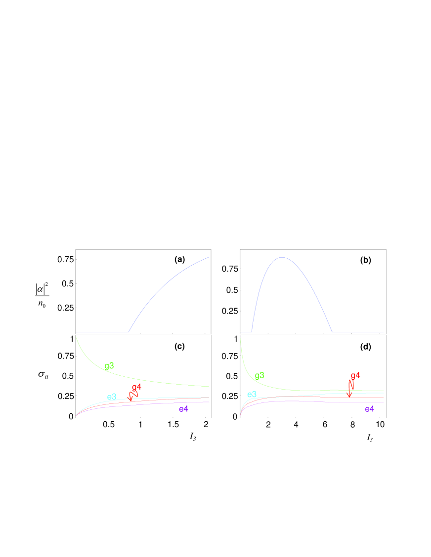
Figure 2: Results from the semiclassical theory as applied to the atom-cavity system in Fig. 1. (a,b) Intracavity intensity $|\alpha|^{2}$ in units of the critical photon number $n_{0}$ is plotted as a function of the pump intensity $I_{3}=(\frac{\Omega_{3}}{2\gamma})^{2}$. A threshold for $|\alpha|^{2}$ is evident for $I_{3}\simeq 0.8$. (c,d) Populations $\sigma_{ii}=\langle\hat{\sigma}_{ii}\rangle$ versus $I_{3}$. In (c), population inversion $\sigma_{e3,e3}>\sigma_{g4,g4}$ occurs over a wide range as the pump intensity $I_{3}$ is increased from $0$, including in the threshold region $I_{3}\simeq 0.8$, with then “population clamping” for $\sigma_{e3,e3}$ as $I_{3}$ increases beyond threshold. In all cases, the recycling intensity $I_{4}=(\frac{\Omega_{4}}{2\gamma})^{2}=3$ and the detunings $\Delta_{AC}=\Delta_{3}=\Delta_{4}=0$.

Examples of the resulting steady-state solutions for the intracavity intensity $|\alpha|^{2}$ together with the populations $\sigma_{ii}$ of the four atomic states are displayed in Figure 2. Parts (a) and (c) of the figure illustrate the behavior of $|\alpha|^{2}$ and $\sigma_{ii}$ around the semiclassical threshold as functions of the pump intensity $I_{3}$. Parts (b) and (d) explore these dependencies over a wider range in $I_{3}$. For fixed ratios among the various decay rates as in Eq. 7, the semiclassical solutions for $|\alpha|^{2}/n_{0}$ as well as the various populations $\sigma_{ii}$ plotted in Fig. 2 depend only on the critical atom number $N_{0}$ (or equivalently, the cooperativity parameter $C_{1}=1/N_{0}$ for a single atom in the cavity). Hence, as emphasized in the Supplementary Information published with our paper Ref. mckeever03b , these steady state solutions from the semiclassical theory are independent of the cavity length $l$, and provide a point of reference for understanding “lasing” for a single atom in a cavity. This is because $N_{0}=\frac{2\kappa\gamma}{g^{2}}$ is independent of cavity length $l$ for a cavity with constant mirror reflectivity and cavity waist $w_{0}$.

Importantly, the semiclassical theory predicts threshold behavior for parameters relevant to our experiment, including inversion $\sigma_{e3,e3}>\sigma_{g4,g4}$ in the threshold region, although this is not essential for Raman gain for $g3\rightarrow g4$ via $e3$. One atom in a cavity can exhibit such a “laser” transition for the steady state solutions in the semiclassical theory because the cooperativity parameter $C_{1}\gg 1$. Indeed, in these calculations we used our experimental value for the cooperativity parameter $C_{1}=1/N_{0}\simeq 12$. Among other relevant features illustrated in Fig. 2 is the quenching of the laser emission around $I_{3}\simeq 6.5$, presumably due to an Autler-Townes splitting of the excited state $e3$ at high pump intensity meyer97a .

III.1 Relationship to a Raman laser

In many respects our system is quite similar to a three-level Raman scheme, for which there is an extended literature (e.g., Ref. eschmann99 and references therein). In fact we have carried out an extensive analysis of a Raman scheme analogous to our system in Fig. 1. Pumping is still done by the field $\Omega_{3}$ on the $3\rightarrow 3^{\prime}$ transition. However, recycling $4\rightarrow 4^{\prime}\rightarrow 3$ by the field $\Omega_{4}$ and decay $\gamma_{34}$ is replaced by direct decay $4\rightarrow 3$ at a fictitious incoherent rate of decay $\beta_{34}$ with level $4^{\prime}$ absent. In all essential details, the results from this analysis are in correspondence with those presented from our four-level analysis in this section. In particular, the threshold onsets in precisely the same fashion as in Fig. 2(a), and the output is “extinguished” at high pump levels for $\Omega_{3}$. This turn-off appears to be associated with an AC-Stark splitting of the excited $3^{\prime}$ level by the $\Omega_{3}$ field that drives the $3^{\prime}\rightarrow 4$ level out of resonance with the cavity due to the splitting of the upper level $3^{\prime}$. Over the range of intensities explored in this section, the “quenching” behavior seems to be unrelated to any coherence effect associated with the combination of the field $\Omega_{4}$ and decay $\gamma_{34}$.

IV Quantum theory for a four-state atom

A one-atom laser operated in a regime of strong coupling has characteristics that are profoundly altered from the familiar case (described e.g. in Refs. carmichael-book ; gardiner-book ), for which the semiclassical equations are supplemented with (small) quantum noise terms. The question then arises as how to recognize a laser in this new regime of strong coupling, where we recall the difficulty that this issue engenders even for systems with critical photon number much greater than unity rice94 ; jin94 ; bjork94 ; protsenko99 . The perspective that we adopt here is to investigate the continuous transformation of a one-atom laser from a domain of weak coupling for which the conventional theory should be approximately valid into a regime of strong coupling for which the full quantum theory is required.

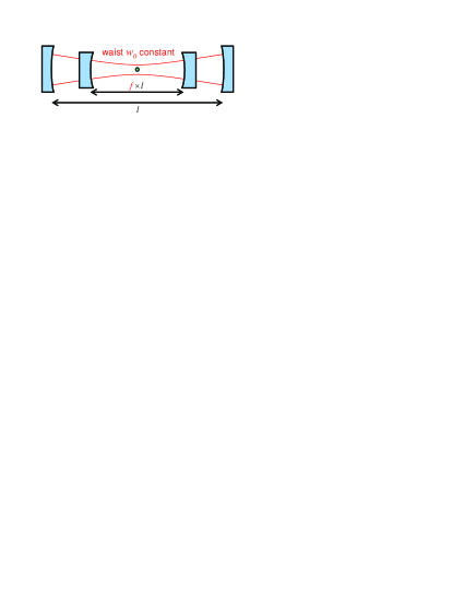
Figure 3: Illustration of the scaling transformation considered in Eqn. 8 whereby the length of a spherical mirror Fabry-Perot cavity is transformed $l\rightarrow fl$ while the cavity waist $w_{0}$ and the atomic position are held constant. The atom is indicated by the “dot” in the center of the cavity mode.

Towards this end, we consider a scenario in which the cavity length (and hence its volume) is gradually reduced from a “large” value for which the conventional theory is valid to a “small” value for which the system is well into a regime of strong coupling. As illustrated in Figure 3 , this transformation is assumed to be under conditions of constant cavity waist $w_{0}$ and mirror reflectivity $R$, in which case scaling the length by a factor $f$ causes the other parameters to scale as follows:

$$l \rightarrow l_{f}=fl,$$ (8)

$$g \rightarrow g_{f}=g/f^{1/2},$$

$$\kappa \rightarrow \kappa_{f}=\kappa/f,$$

$$\gamma \rightarrow \gamma,$$

$$N_{0} \rightarrow N_{0},$$

$$n_{0} \rightarrow n_{0f}=fn_{0}\text{ .}$$

Recall that in the semiclassical theory illustrated in Fig. 2, the quantity $|\alpha|^{2}/n_{0f}$ is invariant under this transformation. By contrast, the role of single photons becomes increasingly important as the cavity length is reduced (i.e., $n_{0f}$ becomes ever smaller), so that deviations from the familiar semiclassical characteristics should become more important, and eventually dominant.

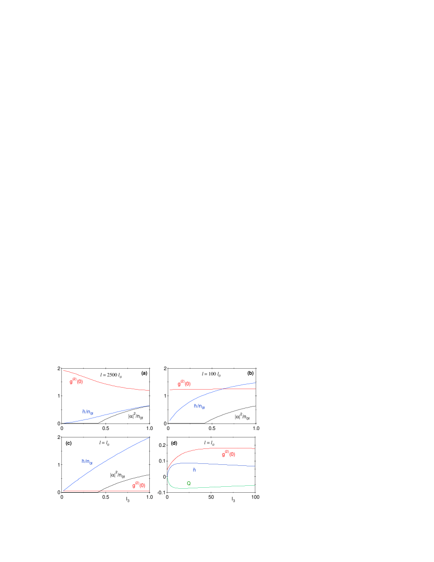
Figure 4: The mean intracavity photon number $\bar{n}/n_{0f}$ (blue) and normalized intensity correlation function $g^{(2)}(0)$ (red) are plotted as functions of pump intensity $I_{3}=(\Omega_{3}/2\gamma)^{2}$ in (a)-(d). In (a)-(c), the cavity length is made progressively shorter ($2500l_{0}$, $100l_{0}$, $l_{0}$), where $l_{0}=42.2~{}\mathrm{\mu m}$ is the length of our actual cavity. The corresponding saturation photon numbers are $n_{0f}=$($33.0$, $1.32$, $0.013$). $\bar{n}/n_{0f}$ and $g^{(2)}(0)$ are calculated from the quantum theory for the four-state system in Fig. 1, while $|\alpha|^{2}/n_{0f}$ given by the black curve is from the semiclassical theory. (d) $\bar{n}$ (blue), $g^{(2)}(0)$ (red), and the Mandel $Q$ parameter (green) shown over an extended range of pump intensity $I_{3}$ for $l=l_{0}$. In all cases, $I_{4}=(\Omega_{4}/2\gamma)^{2}=2$, the $3\rightarrow 4^{\prime}$ and $4\rightarrow 4^{\prime}$ transitions are driven on resonance, and the cavity detuning $\omega_{CA}=0$. Other parameters are as given in the text.

IV.1 Field and atom variables for various cavity lengths

Framed by this perspective, we now present results from the quantum treatment for a four-state model for the atom. Our approach is to obtain steady state results for various operator expectation values directly from numerical solutions of the master equation given in Eq. 2 by way of the Quantum Optics Toolbox written by S. Tan tan99 . Since such numerical methods are by now familiar tools, we turn directly to results from this investigation presented in Figs. 4-9.

These figures display the behavior of various characteristics of the atom-cavity system as the cavity length is reduced from $l=2500l_{0}$ to $l=100l_{0}$ to $l=l_{0}$ to $l=l_{0}/99$, where $l_{0}=42.2\mu$m is the actual length of our cavity. Figure 4 provides an overview of the evolution and is reproduced from the Supplementary Information in Ref. mckeever03b , while Figures 5-9 provide more detailed information about the intracavity field and atomic populations.

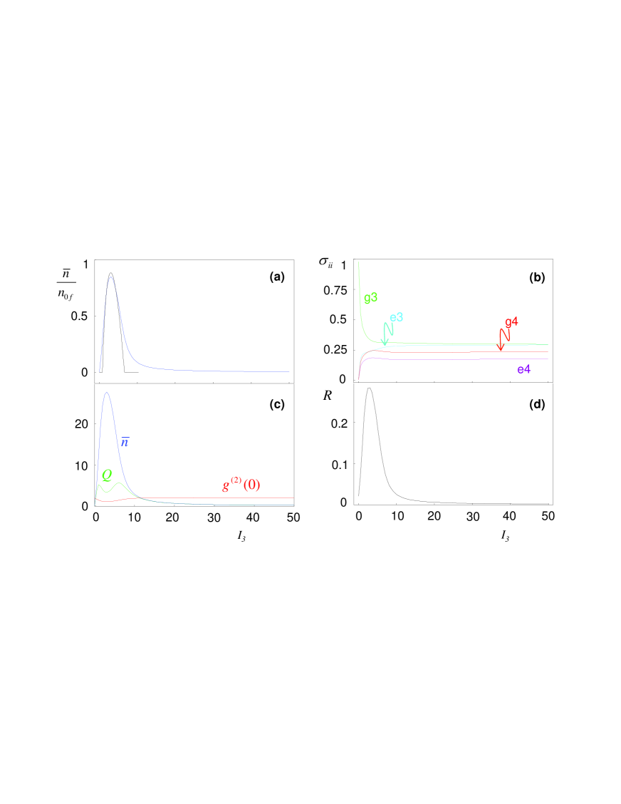
Figure 5: Steady state solutions as functions of pump intensity $I_{3}$ obtained from the numerical solution of the master equation 2 for the four-state atom in a cavity illustrated in Fig. 1. Here, the cavity length $l=2500l_{0}$, where $l_{0}=42.2\mu$m is the cavity length in our experiment. (a) Mean intracavity photon number $\bar{n}$ normalized to the saturation photon number $n_{0f}=33$ (in blue). The corresponding result for $|\alpha|^{2}/n_{0f}$ from the semiclassical theory is given by the black curve. (b) Populations $\sigma_{ii}$ of the four states as labelled. (c) Mean intracavity photon number $\bar{n}$ (blue), Mandel $Q$ parameter (green), and intensity correlation function $g^{(2)}(0)$ (red). (d) Ratio $R$ of photon flux from the cavity mode $\kappa_{f}$ $\bar{n}$ as compared to the rate of atomic fluorescence $\gamma_{43}\sigma_{e3,e3}$ for the excited state $e3$. In all cases, the depleting intensity $I_{4}=(\frac{\Omega_{4}}{2\gamma})^{2}=3$ and the detunings $\Delta_{AC}=\Delta_{3}=\Delta_{4}=0$. Field and atom decay rates are as specified in the text.

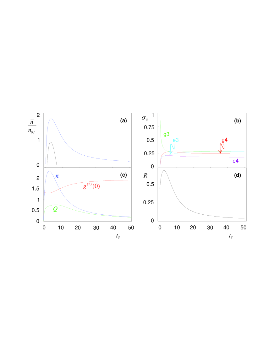
Figure 6: Steady state solutions as functions of pump intensity $I_{3}$ obtained from the numerical solution of the master equation 2 for the four-state atom in a cavity illustrated in Fig. 1. Here, the cavity length $l=100l_{0}$, where $l_{0}=42.2\mu$m is the cavity length in our experiment. (a) Mean intracavity photon number $\bar{n}$ normalized to the saturation photon number $n_{0f}=1.3$ (in blue). The corresponding result for $|\alpha|^{2}/n_{0f}$ from the semiclassical theory is given by the black curve. (b) Populations $\sigma_{ii}$ of the four states as labelled. (c) Mean intracavity photon number $\bar{n}$ (blue), Mandel $Q$ parameter (green), and intensity correlation function $g^{(2)}(0)$ (red). (d) Ratio $R$ of photon flux from the cavity mode $\kappa_{f}$ $\bar{n}$ as compared to the rate of atomic fluorescence $\gamma_{43}\sigma_{e3,e3}$ for the excited state $e3$. In all cases, the depleting intensity $I_{4}=(\frac{\Omega_{4}}{2\gamma})^{2}=3$ and the detunings $\Delta_{AC}=\Delta_{3}=\Delta_{4}=0$. Field and atom decay rates are as specified in the text.

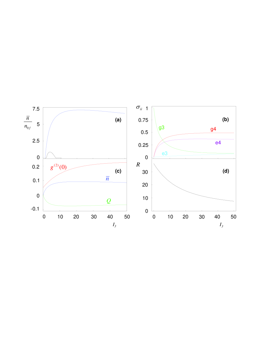
Figure 7: Steady state solutions as functions of pump intensity $I_{3}$ obtained from the numerical solution of the master equation 2 for the four-state atom in a cavity illustrated in Fig. 1. Here, the cavity length $l=l_{0}$, where $l_{0}=42.2\mu$m is the cavity length in our experiment. (a) Mean intracavity photon number $\bar{n}$ normalized to the saturation photon number $n_{0}=0.013$ (in blue). The corresponding result for $|\alpha|^{2}/n_{0}$ from the semiclassical theory is given by the black curve. (b) Populations $\sigma_{ii}$ of the four states as labelled. (c) Mean intracavity photon number $\bar{n}$ (blue), Mandel $Q$ parameter (green), and intensity correlation function $g^{(2)}(0)$ (red). (d) Ratio $R$ of photon flux from the cavity mode $\kappa$ $\bar{n}$ as compared to the rate of atomic fluorescence $\gamma_{43}\sigma_{e3,e3}$ for the excited state $e3$. In all cases, the depleting intensity $I_{4}=(\frac{\Omega_{4}}{2\gamma})^{2}=3$ and the detunings $\Delta_{AC}=\Delta_{3}=\Delta_{4}=0$. Field and atom decay rates are as specified in the text.

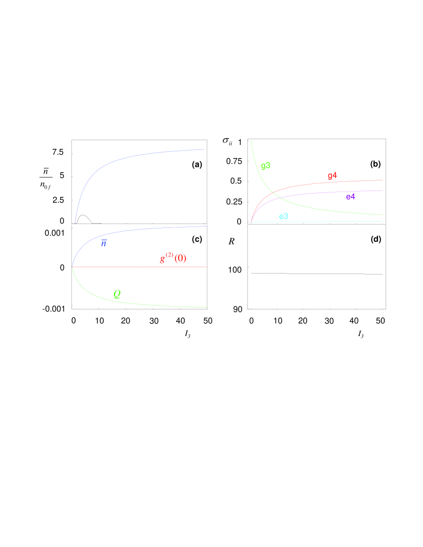
Figure 8: Steady state solutions as functions of pump intensity $I_{3}$ obtained from the numerical solution of the master equation 2 for the four-state atom in a cavity illustrated in Fig. 1. Here, the cavity length $l=l_{0}/99\simeq\lambda_{0}/2$ (i.e., $f=1/99$), where $l_{0}=42.2\mu$m is the cavity length in our experiment and $\lambda_{0}=852.3$ nm is the wavelength of the cavity QED transition. (a) Mean intracavity photon number $\bar{n}$ normalized to the saturation photon number $n_{0f}=1.31\times 10^{-4}$ (in blue). The corresponding result for $|\alpha|^{2}/n_{0f}$ from the semiclassical theory is given by the black curve. (b) Populations $\sigma_{ii}$ of the four states as labelled. (c) Mean intracavity photon number $\bar{n}$ (blue), Mandel $Q$ parameter (green), and intensity correlation function $g^{(2)}(0)$ (red). (d) Ratio $R$ of photon flux from the cavity mode $\kappa_{f}$ $\bar{n}$ as compared to the rate of atomic fluorescence $\gamma_{43}\sigma_{e3,e3}$ for the excited state $e3$. In all cases, the depleting intensity $I_{4}=(\frac{\Omega_{4}}{2\gamma})^{2}=3$ and the detunings $\Delta_{AC}=\Delta_{3}=\Delta_{4}=0$. Field and atom decay rates are as specified in the text.

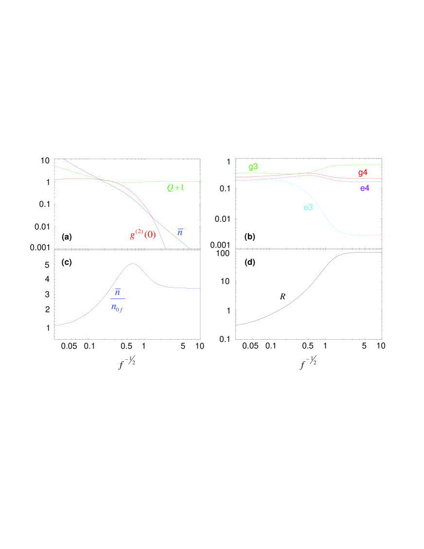
Figure 9: Scaling behavior of various quantities as the cavity length $l$ is varied, where $f=l/l_{0}$, and $l_{0}=42.2$ $\mu$m for our actual cavity. Note that $g\varpropto f^{-1/2}$ and $\kappa\varpropto f^{-1}$ and that the range in $f$ corresponds to that spanned by Figs. 5 to 8, namely $0.01\lesssim f\lesssim 2500$. (a) Mean intracavity photon number $\bar{n}$ (blue), the Mandel $Q$ parameter ($Q+1$ in green), and the intensity correlation function $g^{(2)}(0)$ (red). (b) Populations $\sigma_{ii}$ of the four states as labelled. (c) Mean intracavity photon number $\bar{n}$ normalized to the saturation photon number $n_{0f}=n_{0}f=0.013\times f$. (d) Ratio $R$ of photon flux from the cavity mode $\kappa_{f}\bar{n}$ as compared to the rate of atomic fluorescence $\gamma_{43}\sigma_{e3,e3}$ for the excited state $e3$, where $\kappa_{f}=\kappa/f$. In all cases, the pumping and recycling intensities $I_{3,4}=3$ and the detunings $\Delta_{AC}=\Delta_{3}=\Delta_{4}=0$. Field and atom decay rates are as specified in the text.

Figure 4(a-c) and part (a) in Figs. 5, 6, and 7 display the mean intracavity photon number $\bar{n}/n_{0f}$ (where $n_{0f}$ is calculated for the particular length), and compare this result to $|\alpha|^{2}/n_{0f}$ from the semiclassical theory. The correspondence is close in Figs. 4(a) and 5(a) since $n_{0f}=33$ in this case, but becomes increasingly divergent in Figs. 4(b) and 6(a) for which $n_{0f}=1.3$, and in Figs. 4(c) and 7(a) for which $n_{0f}(f=1)=n_{0}=0.013$ (as in our experiment).

In qualitative terms, the peak in each of the curves for $\bar{n}/n_{0f}$ in Figs. 5, 6, and 7 arises because of a “bottleneck” in the cycle $g3\rightarrow e3\rightarrow g4\rightarrow e4\rightarrow g3$. For our scheme with one atom in a cavity, this cycle can proceed at a rate no faster than that set by the decay rate $\gamma_{34}$. For higher pump intensities $I_{3}$, the quenching of the emission displayed by the semiclassical theory becomes less and less evident with decreasing $l$ as the coherent coupling rate $g$ becomes larger in a regime of strong coupling.

Part (b) in Figs. 5, 6, and 7 shows the populations $\sigma_{ii}$ of the four states. A noteworthy trend here is the rapid reduction of the population $\sigma_{e3,e3}$ with decreasing cavity length. Again, the rate $g$ becomes larger as $l$ is reduced, and eventually overwhelms all other rates, so that population promoted to this state is suppressed.

Figure 4 and part (c) in Figs. 5, 6, and 7 address the question of the photon statistics by plotting the Mandel $Q$ parameter (or equivalently the Fano factor $F=Q+1$) as well as the normalized second-order intensity correlation function $g^{(2)}(0)$ mandel-wolf-95 . As shown in Fig. 4(a), for large $l=2500l_{0}$, the region around the semiclassical threshold displays the familiar behavior associated with a conventional laser gardiner-book ; mandel-wolf-95 ; sargent-book ; haken-book ; scully-zubairy , namely that $g^{(2)}(0)$ evolves smoothly from $g^{(2)}(0)\approx 2$ below the semiclassical threshold to $g^{(2)}(0)\approx 1$ above this threshold. Furthermore, Fig. 5(c) shows that the Mandel $Q$ parameter has a maximum in the region of the threshold rice94 . Beyond this conventional (first) threshold, the Mandel $Q$ parameter in Fig. 5 (c) also exhibits a second maximum, that has been described as a “second” threshold for one-atom lasers meyer97a , and $g^{(2)}(0)$ rises back from $1$ to $2$. With decreasing cavity length, these features are lost as we move into a regime of strong coupling. For example, the two peaks in $Q$ merge into one broad minimum with $Q<0$ indicating the onset of manifestly quantum or nonclassical character for the emission from the atom-cavity system.

Finally, part (d) in Figs. 5, 6, and 7 presents results for the ratio $R$, where

$$R\equiv\frac{\kappa_{f}\bar{n}}{\gamma_{43}\sigma_{e3,e3}}$$ (9)

gives the ratio of photon flux $\kappa_{f}\bar{n}$  from the cavity mode to the photon flux $\gamma_{43}\sigma_{e3,e3}$ appearing as fluorescence into modes other than the cavity mode from the spontaneous decay $e3\rightarrow g4$. For a conventional laser, $\kappa_{f}\bar{n}\ll\gamma_{43}\sigma_{e3,e3}$ below threshold, and $\kappa_{f}\bar{n}\gg\gamma_{43}\sigma_{e3,e3}$ above threshold, with the laser threshold serving as the abrupt transition between these cases in the manner of a nonequilibrium phase transition sargent-book ; scully-zubairy . As illustrated in Fig. 7, no such transition is required in the regime of strong coupling; $R\gg 1$ from the onset as the pump $I_{3}$ is increased. This behavior is analogous to the “thresholdless” lasing discussed in Refs. demartini88 ; jin94 ; bjork94 ; protsenko99 and reviewed by Rice and Carmichael rice94 .

For the system illustrated in Figure 3, the progression in length reduction has a limit at $l=\lambda_{0}/2$ corresponding to a Fabry-Perot cavity with length equal to the lowest order longitudinal mode $\lambda_{0}/2$, where $\lambda_{0}=852.3$ nm is the wavelength of the cavity QED transition. To reach this limit from the length $l_{0}$ appropriate to our actual cavity, we must scale $l_{0}\rightarrow fl_{0}$ with $f=1/99$. In a continuation of the sequence shown in Figs. 5 , 6, and 7, we display in Fig. 8 results for such a cavity with $l=\lambda_{0}/2$. Note that although $C_{1}=1/N_{0}\simeq 12$ is invariant with respect to this scaling and the saturation photon number is reduced to $n_{0f}=1.31\times 10^{-4}$, nevertheless the atom-cavity system has passed out of the domain of strong coupling, even though $(n_{0f},N_{0})\ll 1$. This is because strong coupling requires that $g_{0}\gg(\gamma,\kappa)$, so that $(n_{0},N_{0})\ll 1$ is a necessary but not sufficient condition for achieving strong coupling. For the progression that we are considering with diminishing length (but otherwise with the parameters of our system), $l=\lambda_{0}/2$ does not lie within the regime of strong coupling ($g_{43}/\gamma=61,g_{43}/\kappa=0.40$), but rather more toward the domain of a “one-dimensional atom”, for which $\kappa\gg g^{2}/\kappa\gg\gamma$ (see, for example, Refs. lugiato ; turchette95 for theoretical discussions and a previous experimental investigation). In this domain of the Purcell effect berman94 ; yamamoto-slusher93 ; chang-campillo96 ; vahala03 , the fractional emission into the cavity mode as compared to fluorescent emission into free space for the $3^{\prime}\rightarrow 4$ transition is characterized by the parameter

$$\beta_{43}\equiv\frac{2C_{1}^{(43)}}{1+2C_{1}^{(43)}}\simeq 0.99\text{,}$$ (10)

where $C_{1}^{(43)}=C_{1}\times(\gamma/\gamma_{43})\simeq 48$.

As compared to Figs. 5, 6, and 7, a noteworthy feature of the regime depicted in Fig. 8 is the absence of a dependence of $g^{(2)}(0)$ on the pump level $I_{3}$. In fact, $g^{(2)}(0)\simeq 0$ over the entire range shown, so that the cavity field is effectively occupied only by photon numbers $0$ and $1$. In correspondence to this situation, the Mandel $Q$ parameter in Fig. 8(c) is essentially given by the mean of the intracavity photon number, $Q\simeq-\bar{n}$, with $\bar{n}\ll 1$. Furthermore, the dominance of emission into the cavity mode over fluorescence decay becomes even more pronounced than in Fig. 7(d), as documented by the ratio $R$ in Fig. 8(d). In agreement with expectation set by Eq. 10, note that $R\simeq\beta_{43}/(1-\beta_{43})$. All in all, the “bad-cavity” limit specified by $\kappa\gg g^{2}/\kappa\gg\gamma$ turchette95 ; lugiato (toward which Fig. 8 is pressing) is a domain of single-photon generation for the atom-cavity system, which for $f\ll 1$ has passed out of the regime of strong coupling.

Figures 5, 6, 7, and 8 provide a step-by-step description of the evolution of the atom-cavity system from the domain of conventional laser theory ($l\gg l_{0}$ as in Fig. 5 with $f=2500$), into the regime of strong coupling ($l=l_{0}$ as in Fig. 7 with $f=1$), and then out of the strong-coupling regime into the Purcell domain ($l=l_{0}/99\simeq\lambda_{0}/2$ as approached in Fig. 8 with $f=0.01$) berman94 ; yamamoto-slusher93 ; chang-campillo96 ; vahala03 . We now attempt to give a more global perspective of the scaling behavior of the atom-cavity system by examining various field and atomic variables directly as functions of the scale parameter $f=l/l_{0}$. A particular set of such results is displayed in Figure 9, where the pump intensity $I_{3}=3$ is fixed near the peak in the output from the semiclassical theory in Fig. 2, and the recycling intensity $I_{4}$ is held constant at $I_{4}=3$.

In Fig. 9(a) the mean intracavity photon number $\bar{n}$ is seen to undergo a precipitous drop as the cavity length is made progressively shorter (i.e., increasing $f^{-1/2}$, since $l\varpropto f$). However, when $\bar{n}$ is normalized to the critical photon number $n_{0f}$ , the quantity $\bar{n}/n_{0f}$ is seen to approach unity for small $f^{-1/2}$ (i.e., long cavities with $l\gg l_{0}$) as appropriate to the conventional theory in Fig. 5). With increases in $f^{-1/2}$ (i.e., shorter cavity lengths), $\bar{n}/n_{0f}$ rises to a maximum around $f\sim 3$ for strong coupling with $l\sim l_{0}$ as in Fig. 7, before then decreasing to approach a constant value for yet larger values of $f^{-1/2}$ as the system exits from the domain of strong coupling.

Also shown in Fig. 9(a) are the quantities $g^{(2)}(0)$ and $Q+1$ that characterize the photon statistics of the intracavity field. As previously noted, $g^{(2)}(0)$ lies in the range $1\leq g^{(2)}(0)\leq 2$ for conventional laser theory, but drops below unity in the regime of strong coupling and approaches zero for $f\ll 1$. In this same limit of very small cavities in the Purcell regime, $Q\simeq-\bar{n}$.

Fig. 9(b) displays the populations for the four-state system as functions of $f^{-1/2}$. For the conventional regime with $f^{-1/2}\ll 1$ , there is population inversion, $\sigma_{e3,e3}>\sigma_{g4,g4}$ (which was shown in Fig. 2 for small values of $I_{3}$), but this possibility is lost for increasing $f^{-1/2}$ (i.e., decreasing cavity length). Strong coupling dictates that the rate $g$ dominates all others, so that appreciable population cannot be maintained in the state $e3$. Finally, Fig. 9(d) displays the dependence of the ratio $R=(\kappa_{f}\bar{n})/(\gamma_{43}\sigma_{e3,e3})$ on $f^{-1/2}$. From values $R<1$ in the conventional domain, $R$ rises monotonically with decreasing cavity length reaching the plateau $R\gg 1$ specified by Eq. 10.

IV.2 Vacuum-Rabi splitting

In the preceding discussion, we have compared various aspects of our one-atom system with conventional lasers and have restricted the analysis to the case of resonant excitation with $\Delta_{3}=0$. Our actual system operates in a regime of strong coupling, so that there should be an explicit manifestation of the “vacuum-Rabi” splitting associated with one quantum of excitation in the $4\leftrightarrow 3^{\prime}$ manifold eberly83 ; agarwal84 ; thompson92 .

To investigate this question, we consider the dependence of the average intracavity photon number $\bar{n}$ on the detuning $\Delta_{3}$ of the pump field $\Omega_{3}$, with the result of this analysis illustrated in Fig. 10. For weak excitation $I_{3}\lesssim 1$ (well below the peak in Fig. 7(a)), the intracavity photon $\bar{n}$ is maximized around $\Delta_{3}=\pm g_{43}$ (and not at $\Delta_{3}=0$) in correspondence to the eigenvalue structure for the $g4\leftrightarrow e3$ manifold in presence of strong coupling. The excited state $e3$ is now represented by a superposition of the nondegenerate states $|\psi_{\pm}\rangle$ whose energies are split by the coupling energy $\pm\hbar g_{43}$ . However, for large pump intensities $I_{3}\sim 10$, this splitting is lost as the Autler-Townes effect associated with the pump field on the $g3\leftrightarrow e3$ transition grows to exceed $g_{43}$.

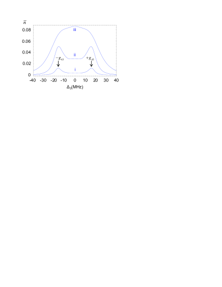
Figure 10: The mean intracavity photon number $\bar{n}$ versus the detuning $\Delta_{3}$ (in cycles/sec) of the pump field $\Omega_{3}$, where $\Delta_{3}=0$ corresponds to the transition frequency $\omega_{33}$. The three curves are for increasing pump intensity (i) $I_{3}=0.1$, (ii) $I_{3}=1.0$, (iii) $I_{3}=10.0$. The arrows indicate the positions of the expected “vacuum-Rabi” peaks at $\pm g_{43}$, where $g_{43}/2\pi=16$ MHz. In all cases, the recycling field $\Omega_{4}$ is on resonance $\Delta_{4}=0$ and has intensity $I_{4}=3$.

IV.3 Optical spectrum of the cavity emission

A central feature of a conventional laser is the optical spectrum of the emitted field, defined by

$$\Phi(\Omega)\equiv\int_{-\infty}^{+\infty}d\tau\{\lim\limits_{t\rightarrow\infty}\langle\hat{a}^{\dagger}(t)\hat{a}(t+\tau)\rangle\}\exp(-i\Omega\tau)\text{ ,}$$ (11)

where as in Eq. 1, $(\hat{a}^{\dagger},\hat{a})$ are the creation and annihilation operators for the single-mode field of the cavity coupled to the atomic transition $e3\leftrightarrow g4$. The results for the Schawlow-Townes linewidth are well-known and will not be discussed here carmichael-book ; gardiner-book ; sargent-book ; haken-book ; scully-zubairy . Instead, in Fig. 11 we present results specific to the domain of operation of our system.

For the choice of parameters corresponding to Fig. 7, $\Phi(\Omega)$ in Fig. 11(a) exhibits a pronounced two-peak structure, with the positions of the peaks corresponding to the Autler-Townes splitting of the ground state by the recycling field $\Omega_{4}$. Contrary to what might have been expected from the analysis of the previous section, $\Phi(\Omega)$ shows no distinctive features associated with the vacuum-Rabi splitting of the excited state. For reduced values of pumping and recycling intensities $I_{3,4}=0.5$, there are small features in the optical spectrum at $\Omega\approx\pm g_{43}$, as is illustrated in Fig. 11 when $\Phi(\Omega)$ is plotted on logarithmic scale. With respect to the complex degree of coherence mandel-wolf-95 , the coherence properties of the light from the one-atom laser in the regime of strong coupling are set simply by the inverse of the spectral width of $\Phi(\Omega)$, which can be determined from the plots in Fig. 11.

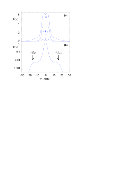
Figure 11: The optical spectrum $\Phi(\nu)$ as a function of frequency offset $\nu$ (in cycles/sec, $\Omega=2\pi\nu$), where $\nu=0$ corresponds to the transition frequency $\omega_{43}$. (a) Three spectra $\Phi(\nu)$ for increasing pump intensity (i) $I_{3}=0.1$, (ii) $I_{3}=1.0$, (iii) $I_{3}=10.0,$ with the recycling intensity $I_{4}=3$ in all cases. The overall normalization of $\Phi(\nu)$ is arbitrary, but is common for the three cases. (b) $\Phi(\nu)$ on a logarithmic scale for decreased intensities $I_{3}=I_{4}=0.5$, with the peak value of $\Phi$ scaled to unity. The arrows indicate the position of the expected “vacuum-Rabi” peaks at $\pm g_{43}$, where $g_{43}/2\pi=16$ MHz. In all cases in (a) and (b), the pumping field $\Omega_{3}$ and the recycling field $\Omega_{4}$ are on resonance with their respective transitions ($\Delta_{3}=0=\Delta_{4}$).

The curves shown in Fig. 11 are calculated by way of the quantum regression theorem applied to the four-state system of Fig. 1. From the quantum regression theorem, we have that the two time correlation function in Eq. 11 is given by

$$\langle a^{\dagger}(0)a(\tau)\rangle=Tr[\rho_{ss}a^{\dagger}(0)a(\tau)]=Tr[\rho(\tau)a(0)]$$

where $\rho(\tau)$ is obtained by numerically evolving

$$\rho_{0}=\rho_{ss}a^{\dagger}(0)$$

under the master equation, and $\rho_{ss}$ is the steady state density matrix. By Fourier transforming the correlation function according to Eq. 11, we obtain the optical spectrum.

The optical spectrum of the emitted light from our cavity could in principle be measured by way of heterodyne detection. The cavity output would be combined on a highly transmissive beam splitter with a local oscillator beam that is frequency shifted by an interval $\Delta\omega$ that is large compared to the range of frequencies in the output field. The optical spectrum is then obtained by taking the Fourier transform of autocorrelation function of the resulting heterodyne current. Although we have not carried out this procedure experimentally, it is straightforward to model using a quantum jumps simulation of the four state model. We have computed such spectra for several values of $I_{3}$, using a local oscillator flux equal to $\kappa$. This is an experimentally reasonable value, since it is small enough so as to not saturate the detectors, yet large enough that, as our further simulations indicate, increasing the flux does not significantly change the resulting spectrum. The results for the spectrum obtained from this quantum jumps simulation agree reasonably well with results from the quantum regression theorem presented in Fig. 11.

V Quantum theory including Zeeman states and two cavity modes

In an attempt to provide a more detailed quantitative treatment of our experiment, we have developed a model that includes all of the Zeeman states $(F,m_{F})$ for the $F=3,4$ ground levels and the $F^{\prime}=3^{\prime},4^{\prime}$ excited levels of the $6S_{1/2}\leftrightarrow 6P_{3/2}$ transition in atomic Cesium, of which there are $32$ in total. We also include two cavity modes with orthogonal linear polarizations to describe the two nearly degenerate $TEM_{00}$ modes of our cavity mckeever03 , with three Fock states for each mode $\{|0\rangle,|1\rangle,|2\rangle\}$. The total dimension of the Hilbert space for this set of atomic and field states is then $d=32\times 3\times 3=288$, making it impractical to obtain steady state solutions from the master equation directly. Instead, we employ the Quantum Optics Toolbox tan99 to implement a quantum jumps simulation, with various expectation values computed from the stochastic trials.

In broad outline, our expanded model includes Hamiltonian terms of the form of Eq. 1, with now the terms $\hat{\sigma}_{ij}$ generalized to incorporate each of the various Zeeman states. Likewise, the coherent coupling of the atom to the cavity takes into account two orthogonally polarized modes $(\hat{a},\hat{b})$. The operators $\hat{L}_{i}$ are similarly modified to obtain a new master equation that includes the full set of decay paths among the various states (i.e., $\sigma_{\pm},\pi$ transitions), as well as the associated quantum collapse terms in the simulation.

We attempt to describe the dynamics arising from the complex state of spatially varying polarization associated with the $\Omega_{3,4}$ beams by way of the following simple model. In a coordinate system with the $x,z$ directions perpendicular to the cavity axis along $y$, the $\Omega_{3,4}$ beams propagate along $x,z$ with orthogonal $\sigma_{\pm}$ configurations. The helical patterns of linear polarization from pairs of counter-propagating beams then give rise to terms in the interaction Hamiltonians $\hat{H}_{2,3}$ of the form

$$\hat{H}_{2} = \frac{1}{2\sqrt{2}}\Omega_{3}[(\hat{\Sigma}_{g3,e3}^{z}+\hat{\Sigma}_{e3,g3}^{z})\sin(\theta_{3x})$$

$$+(\hat{\Sigma}_{g3,e3}^{x}+\hat{\Sigma}_{e3,g3}^{x})\sin(\theta_{3z})]$$

$$+\frac{1}{2}\Omega_{3}[(\hat{\Sigma}_{g3,e3}^{y}+\hat{\Sigma}_{e3,g3}^{y})(\cos(\theta_{3x})+\cos(\theta_{3z}))]$$

and similarly for $\hat{H}_{3}$ to describe the $\Omega_{4}$ beams with independent phases $(\theta_{4x},\theta_{4z})$. Here $\Omega_{3}$ and $\Omega_{4}$ are Rabi frequencies corresponding to the incoherent sum of the intensities of the four individual beams. In Eq. V, the operators $\hat{\Sigma}_{g3,e3}^{x,y,z}$ are linear combinations of various atomic projection operators for the diverse Zeeman-specific transitions for linear polarization along $x,y,z$, and are given explicitly by

$$\hat{\Sigma}^{x}_{g3,e3} = -\frac{1}{\sqrt{2}}(\hat{\Sigma}^{+1}_{g3,e3}-\hat{\Sigma}^{-1}_{g3,e3})$$ (13)

$$\hat{\Sigma}^{y}_{g3,e3} = \frac{i}{\sqrt{2}}(\hat{\Sigma}^{+1}_{g3,e3}+\hat{\Sigma}^{-1}_{g3,e3})$$ (14)

$$\hat{\Sigma}^{x}_{g3,e3} = \hat{\Sigma}^{0}_{g3,e3}$$ (15)

where

$$\hat{\Sigma}^{q}_{g3,e3}=\sum_{m}\sum_{m^{\prime}}|g3,m\rangle\langle 3,m;1,q|4,m^{\prime}\rangle\langle g4,m^{\prime}|$$ (16)

The phases $\theta_{i}$ arise from the spatial variations of the polarization state of the $\Omega_{3,4}$ beams, and are given, for example, by $\theta_{3x}=k_{3x}x$ with $k_{3x}$ as the wave vector of the pair of $\Omega_{3}$ beams propagating along $x$.

The $\Omega_{3,4}$ beams tend to optically pump the atom into dark states, with this pumping counterbalanced by atomic motion leading to cooling boiron96 and by any residual magnetic field. In our case, imperfections in the FORT polarization hood01 ; mckeever03 result in a small pseudo-magnetic field along the cavity axis $y$ corwin99 with peak magnitude $B_{y}^{F}\simeq 0.75$ G. This pseudo-field $B_{y}^{F}$ is included in our simulations and tends to counteract optical pumping by the $\Omega_{3,4}$ beams into dark states for linear polarization in the $x-z$ plane, $\theta_{3x}=\theta_{3z}=\theta_{4x}=\theta_{4z}=\pi/2$, but has no effect for polarization along the cavity axis $y$, $\theta_{3x}=\theta_{3z}=\theta_{4x}=\theta_{4z}=0$.

Overall, the operation of our driven atom-cavity system involves an interplay of cycling through the levels $g3\rightarrow e3\rightarrow g4\rightarrow e4\rightarrow g3$ to achieve output light on the $e3\rightarrow g4$ transition, and of polarization gradient cooling for extended trapping times. This latter process involves atomic motion through the polarization gradients of the $\Omega_{3,4}$ beams and is greatly complicated by the presence of $B_{y}^{F}$. The detunings and intensities of the $\Omega_{3,4}$ beams are chosen operationally such as to optimize the output from our one-atom laser in a regime of strong coupling, while at the same time maintaining acceptable trapping times, as shown in Fig. 2 of Ref. mckeever03b .

V.1 Mean intracavity photon number as a function of pump intensity

In this section, we present simulation results for the mean intracavity photon number versus pump intensity. In qualitative terms, we should expect that the output flux $\kappa\bar{n}$ predicted from the full multi-state model is significantly below that calculated from the four-state model presented in Section IV. This is because the atom necessarily spends increased time in manifolds of dark states associated with the pumping by the $\Omega_{3,4}$ beams.

We can modify the four level model to account for these effects by reducing the decay rate $\gamma_{34}\rightarrow\gamma_{34}^{\prime}$. The slower cycling of the atom due to the reduction of $\gamma_{34}^{\prime}$ approximates, in a phenomenological way, the slowing effect on the recycling of the atom due to optical pumping into dark states. We find that a value $\gamma_{34}^{\prime}=0.07\times\gamma_{34}$ gives a good fit to the data (Fig. 12(a,b)). We plot the intracavity photon number versus $x\equiv(7/9)(I_{3}/I_{4})$, since we estimate that either measured intensity alone is uncertain by a factor of about $2$, but the ratio is known much more accurately.

For the multi-level simulation, we use two different models to generate mean intracavity photon number versus pump intensity curves. In the first model, we neglect the motion of the atom and attempt to capture the essential features of the optical pumping processes via a single constant phase $\theta=\theta_{3x}=\theta_{3z}=\theta_{4x}=\theta_{4z}$. The choice $\theta=0$ gives no output light, since the $\Omega_{3,4}$ beams pump the atom into dark states. The value $\theta=\pi/2$ chosen for the comparison in Fig. 12(c,d) gives good correspondence between the simulations and our measurements with the adjustment of no other parameters. For this curve, we plot the average $(\bar{n}_{a}+\bar{n}_{b})/2$ of the intracavity field for the two cavity modes $a$ and $b$.

As a second, more sophisticated model, we assume that the atom moves at a constant velocity in the radial direction. This gives time dependent phases; for example, if we assume that the $x$ coordinate of the atom is

$$x(t)=x_{0}+v_{x}t$$

then

$$\theta_{3x}(t)=k_{3x}x=\theta_{3x,0}+\omega_{3x}t$$

where $\theta_{3x,0}=k_{3x}x_{0}$, $\omega_{3x}=k_{3x}v_{x}$. For a single simulation run we randomly choose the velocity of the atom and initial phases of the $\Omega_{3,4}$ pumping beams; the intensities from 20 such runs are averaged for each value of $x$. The velocities are chosen uniformly in the range $10-20cm/s$, which gives angular frequencies in the range $2\pi 100-200kHz$. The resulting input/output curve is plotted in Fig 12(e,f). As before, we plot the average of the intracavity field for the two cavity modes.

We make no claim for detailed quantitative agreement between theory and experiment, as the simulations are sensitive to the parameters which are known only approximately, such as the intensity of the $\Omega_{3,4}$ pumping beams and the magnitude of the pseudo and real magnetic fields. Also, the simulations neglect a number of features of the real system, such as atomic motion in the axial direction, the dependence of the cavity coupling $g$ on the position of the atom, and a possible intensity imbalance in the $\Omega_{3,4}$ pumping beams. However, the simulations do support the conclusion that the range of coupling values $g$ that contribute to our results is restricted roughly to $0.5g_{0}\lesssim g\lesssim g_{0}$. Furthermore, the simulations yield information about the atomic populations, from which we deduce that the rate of emission from the cavity $\kappa\bar{n}$ exceeds that by way of fluorescent decay $3^{\prime}\rightarrow 4$, $\gamma_{43^{\prime}}\langle\sigma_{3^{\prime}3^{\prime}}\rangle$, by roughly tenfold over the range of pump intensity $I_{3}$ shown in Fig. 12a.

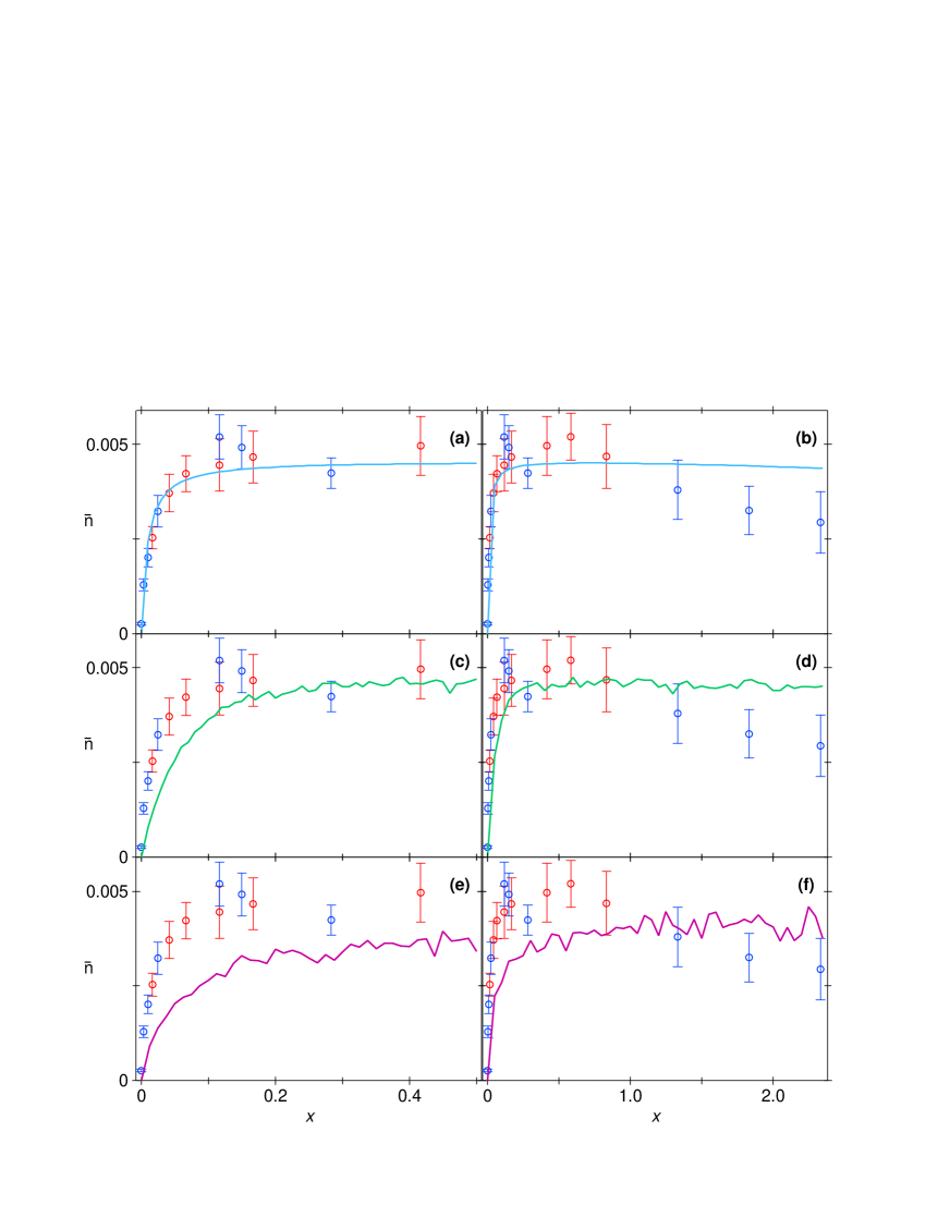
Figure 12: Comparison of theory and experiment for the intracavity photon number $\bar{n}$ as a function of pump intensity $x\equiv(7/9)(I_{3}/I_{4})$ for fixed $I_{4}=13$ (corresponding to a measured intensity of $50mW/cm^{2}$ ). The measurements (points with error bars) are from Figure 3 of Ref. mckeever03b . (a,b) $\bar{n}$ versus pump strength $x$ for the four level model with $\gamma_{43}^{\prime}=0.07\times\gamma_{43}$. (c,d) $\bar{n}$ versus pump strength $x$ for the constant phase model with $\theta=\pi/2$. (e,f) $\bar{n}$ versus pump strength $x$ for the constant velocity model described in the text. The immediate onset of emission supports the conclusion of “thresholdless” lasing. Two independent sets of measurements are shown as the red and blue points, and agree reasonably well with each other. Details of the measurements can be found in Ref. mckeever03b , while the parameters for the simulation are given in the text.

V.2 Photon statistics as expressed by the intensity correlation function $g^{(2)}(\tau)$

In addition to measurements of $\bar{n}$ versus pumping rate, we have also investigated the photon statistics of the light emitted by the TEM₀₀ mode of the cavity by way of the two single-photon detectors D_1,2 illustrated in Fig. 1 of Ref. mckeever03b . From the cross-correlation of the resulting binned photon arrival times and the mean counting rates of the signals and the background, we construct the normalized intensity correlation function (see the Supplementary Information accompanying Ref. mckeever03b )

$$g^{(2)}(\tau)=\frac{\langle:\hat{I}(t)\hat{I}(t+\tau):\rangle}{\langle:\hat{I}(t):\rangle^{2}}\text{ ,}$$ (17)

where the colons denote normal and time ordering for the intensity operators $\hat{I}$ mandel-wolf-95 .

Two measurements for $g^{(2)}(\tau)$ from Figure 4 of Ref. mckeever03b are reproduced in (a,b) of Figs. 13 and 14, together with results from our quantum jumps simulation from the constant phase model with $\theta=\pi/2$, in (c,d). In Fig. 13, we again have $I_{4}\simeq 13$ and the pump intensity $I_{3}$ is set for operation with $x\simeq 0.17$ near the “knee” in $\bar{n}$ versus $x$, while in Fig. 14, the pump level is increased to $x\simeq 0.83$. These measurements demonstrate that the light from the atom-cavity system is manifestly quantum (i.e., nonclassical) and exhibits photon antibunching $g^{(2)}(0)<g^{(2)}(\tau)$ and sub-Poissonian photon statistics $g^{(2)}(0)<1$ mandel-wolf-95 . In agreement with the trend predicted by the four-state model in Fig. 7(c) (as well as by the full quantum jumps simulation), $g^{(2)}(0)$ increases with increasing pump intensity, with a concomitant decrease in these nonclassical effects. The bottleneck associated with the recycling process leads to this nonclassical character, since detection of a second photon given the first detection event requires that the atom be recycled from the $F=4$ ground state back to the $F=3$ ground. In this regard, we point to the prior work on pump-noise suppressed lasers in multi-level atomic systems, as for example, in Ref. ritsch91 .

In more quantitative terms, theoretical results for $g^{(2)}(\tau)$ from the full quantum jumps simulation are given in parts (c,d) of Figs. 13 and 14 for $x=0.17$ and $x=0.83$. The excess fluctuations $g^{(2)}(\tau)\gtrsim 1$ extending over $\tau\simeq\pm 1~{}\mathrm{\mu s}$ appear to be related to the interplay of atomic motion and optical pumping into dark states boiron96 , as well as Larmor precession that arises from residual ellipticity in polarization of the intracavity FORT mckeever03 ; corwin99 .

These results for $g^{(2)}(\tau)$ provide a perspective on the issue of whether the cavity is effectively “empty” since $\bar{n}$ is quite small. Based upon the mean photon flux from the cavity, this is a reasonably inference, but it is also misleading. The nonzero values for $g^{(2)}(\tau=0)\simeq 0.3,0.6\gg 0.01$ in Figs. 13 and 14 are in fact due to the presence of more than one photon in the cavity. Although the mean intracavity photon number is only $\bar{n}\sim 0.005$, this number is comparable to the saturation photon number $n_{0}\simeq 0.013$. Indeed, the quantum statistical character of the intracavity field is determined from the self-consistent interplay of atom and cavity field as in standard laser theories, even though it might appear as this interplay is not relevant to the determination of a dynamic steady state. Figure 9 attempts to illustrate this point by investigating the passage from the domain of conventional laser theory through the regime of strong coupling and thence into a domain of single photon generation with $g^{(2)}(\tau=0)\simeq 0$ over the entire range of pumping conditions.

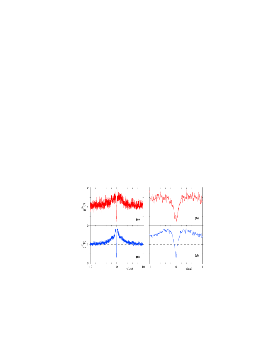
Figure 13: The intensity correlation function $g^{(2)}(\tau)$ of the one-atom laser. (a,b) $g^{(2)}(\tau)$ for $x\simeq 0.17$ as experimentally determined in Ref. mckeever03b . (c,d) Theoretical result for $g^{(2)}(\tau)$ for $x=0.17$ from a quantum jumps simulation with $\theta=\pi/2$. All traces have been “smoothed” by convolution with a Gaussian function of width $\sigma=5~{}\mathrm{ns}$.

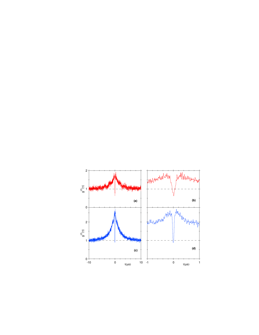
Figure 14: The intensity correlation function $g^{(2)}(\tau)$ of the one-atom laser. (a,b) $g^{(2)}(\tau)$ for $x\simeq 0.83$ as experimentally determined in Ref. mckeever03b . (c,d) Theoretical result for $g^{(2)}(\tau)$ for $x=0.83$ from a quantum jumps simulation with $\theta=\pi/2$. All traces have been “smoothed” by convolution with a Gaussian function of width $\sigma=5~{}\mathrm{ns}$.

V.3 Discussion of possible coherence effects

In Section IIIA we briefly described our analysis of an equivalent Raman scheme to address the question of possible coherence effects associated with the $\Omega_{4}$ recycling beam. Beyond this analysis, we have also considered the possibility that various other coherent processes associated with the pump fields might be important. One concern relates to the possibility that $4$-wave mixing processes could be important, as for example, in a wave-mixing process that cycles the atom $3\rightarrow 3^{\prime}\rightarrow 4\rightarrow 4^{\prime}\rightarrow 3$ gauthier03 . From an operational perspective, if there were to be a correlated process involved in the cycling of the atom $3\rightarrow 3^{\prime}\rightarrow 4\rightarrow 4^{\prime}\rightarrow 3$, then two photons would be emitted into the cavity mode (the “signal” on the $3^{\prime}\rightarrow 4$ transition and the “idler” on the $4^{\prime}\rightarrow 3$ transition). In this case since we employ no filter to block the “idler” field separated by $9.2$GHz, the measured intensity correlation function $g^{(2)}(\tau)$ for the emitted light from the cavity would exhibit bunching around $\tau=0$, instead of the observed antibunching and sub-Poissonian character. The measured character of $g^{(2)}(\tau)$ therefore argues against a coherent process that cycles the atom from an initial quantum state and back to that state by way of coherent processes involving coupling to the cavity field.

We also note that the coherent coupling of the cavity field and atom for the $4^{\prime}\rightarrow 3$ transition is greatly suppressed due to the large detuning $\simeq 9.2$GHz, leading to an effective coupling coefficient $(g_{eff}/2\pi\sim 30$ kHz$)\ll(\gamma_{\|}/2\pi\simeq 5.2$ MHz$)$. Therefore, for whatever mixing processes, the coupling to the external vacuum modes characterized by the rate $\gamma_{\|}$ should dominate that due to $g_{eff}$. In this regard, note that we have included the effect of off-resonant coupling of the $4^{\prime}$ excited state in our simulations (which is only $\simeq 200$ MHz detuned). The relevant process is then excitation $4\rightarrow 4^{\prime}$ via the $\Omega_{4}$ pump field, followed by emission into the cavity mode due to the coherent coupling of the transition $4^{\prime}\rightarrow 4$. This coupling increases the intracavity photon number by only about $10\%$, suggesting that coupling for the $4^{\prime}\rightarrow 3$ transition $9.2$ GHz away is negligible.

In support of these comments, our detailed numerical simulations agree sensibly well with the observed behavior of $g^{(2)}(\tau)$ (as in Figures 13 and 14), and do not include any “wave-mixing” effects. This statement is likewise valid for the dependence of photon number versus pump level $\Omega_{3}^{2}$. Furthermore, as previously discussed, the model calculation for a four-state system agrees well in its essential characteristics with a three-state system where the decay of the ground state $4\rightarrow 3$ is via an ad hoc spontaneous process (as in a Raman laser) rather than by pumping $4\rightarrow 4^{\prime}$ and decay $4^{\prime}\rightarrow 3$.

A final general comment relates to the nature of phase-matching (e.g., as applied to $4$-wave mixing and parametric down conversion) for a single atom in a cavity. For a sample of atoms (or a crystal), there is a geometry that defines directions for which fields from successive atoms might add constructively for various waves (e.g., pump, signal, idler). Cavities can then be placed around these directions to enhance the processes (e.g., the threshold for an optical parametric oscillator is reduced by a factor of the square of the cavity finesse for resonant enhancement of both signal and idler fields). Clearly a cavity would be ineffective if its geometry did not match the preferred geometry defined by the sample and pump beams. However, for a single atom as in our experiment, these considerations do not apply in nearly the same fashion. The relevant issues are the coherent coupling coefficients $g_{ij}$ of the various atomic transitions to the cavity field.

VI Summary

We have presented a simplified four-level model which describes the qualitative features of our experiment. We have shown how decreasing the cavity length causes the model system to move from a regime of weak coupling, where the semiclassical laser theory applies, into a regime of strong coupling, where quantum deviations become important. The four-state model predicts many of the observed features of our experimental system, including the qualitative shape of the intracavity photon number versus pumping intensity curve, and photon antibunching.

In addition, to predict quantitative values for comparison with our experimental results, we have developed a full multi-level model which correctly describes optical pumping and Larmor precession effects within the Zeeman substructure. We have shown that these effects play an important role in describing the observed input/ output characteristics of the system, and that by including a simple model for the motion of the atom we can obtain reasonable agreement with the experimentally observed curve. We have also used the simulation to calculate intensity correlation functions, and have compared these results to measurements of $g^{(2)}(\tau)$ from our experiment.

We gratefully acknowledge interactions with K. Birnbaum, L.-M. Duan, D. J. Gauthier, T. Lynn, T. Northup, A. S. Parkins, and D. M. Stamper-Kurn. This work was supported by the National Science Foundation, by the Caltech MURI Center for Quantum Networks under ARO Grant No. DAAD19-00-1-0374, and by the Office of Naval Research.

References

- (1) J. McKeever, A. Boca, A. D. Boozer, J. R. Buck, and H. J. Kimble, Nature (London) 425, 268 (2003).
- (2) Y. Mu and C. M. Savage, Phys. Rev. A 46, 5944 (1992).
- (3) C. Ginzel, H.-J. Briegel, U. Martini, B.-G. Englert, and A. Schenzle, Phys. Rev. A 48, 732 (1993).
- (4) T. Pellizzari and H. Ritsch, Phys. Rev. Lett. 72, 3973 (1994).
- (5) T. Pellizzari and H. Ritsch, J. Mod. Opt. 41 , 609 (1994).
- (6) P. Horak, K. M. Gheri, and H. Ritsch, Phys. Rev. A 51, 3257 (1995).
- (7) H.-J. Briegel, G. M. Meyer, and B.-G. Englert, Phys. Rev. A 53, 1143 (1996).
- (8) G. M. Meyer, H.-J. Briegel, and H. Walther, Europhys. Lett. 37, 317 (1997).
- (9) M. Löffler, G. M. Meyer, and H. Walther, Phys. Rev. A 55, 3923 (1997).
- (10) G. M. Meyer, M. Löffler, and H. Walther, Phys. Rev. A 56, R1099 (1997).
- (11) G. M. Meyer and H.-J. Briegel, Phys. Rev. A 58, 3210 (1998).
- (12) B. Jones, S. Ghose, J. P. Clemens, P. R. Rice, and L. M. Pedrotti, Phys. Rev. A 60, 3267 (1999).
- (13) Y.-T. Chough, H.-J. Moon, H. Nha, and K. An, Phys. Rev. A 63, 013804 (1996).
- (14) C. Di Fidio, W. Vogel, R. L. de Matos Filho, and L. Davidovich, Phys. Rev. A 65, 013811 (2001).
- (15) S. Ya. Kilin and T. B. Karlovich, JETP 95, 805 (2002).
- (16) J. P. Clemens, P. R. Rice, and L. M. Pedrotti (2003).
- (17) T. Salzburger and H. Ritsch, quant-ph/0312181.
- (18) F. De Martini and G. R. Jacobivitz, Phys. Rev. Lett. 60, 1711 (1988).
- (19) P. R. Rice and H. J. Carmichael, Phys. Rev. A 50, 4318 (1994).
- (20) R. Jin, D. Boggavarapu, M. Sargent III, P. Meystre, H. M. Gibbs, and G. Khitrova, Phys. Rev. A 49, 4038 (1994).
- (21) G. Björk, A. Karlsson, and Y. Yamamoto, Phys. Rev. A 50, 1675 (1994).
- (22) I. Protsenko, P. Domokos, V. Lefevre-Seguin, J. Hare, J. M. Raimond, and L. Davidovich, Phys. Rev. A 59, 1667 (2001).
- (23) J. J. Sanchez-Mondragon, N. B. Narozhny, and J. H. Eberly, Phys. Rev. Lett. 51, 550 (1983).
- (24) G. S. Agarwal, Phys. Rev. Lett. 53, 1732 (1984).
- (25) R. J. Thompson, G. Rempe, and H. J. Kimble, Phys. Rev. Lett. 68, 1132 (1992).
- (26) Cavity Quantum Electrodynamics, edited by P. Berman (Academic Press, San Diego, 1994).
- (27) Cavity Quantum Optics and the Quantum Measurement , P. Meystre, in Progress in Optics, Vol. XXX edited by E. Wolf (Elsevier Science Publishers B.V., Amsterdam, 1992), pp. 261-355.
- (28) Y. Yamamoto and R. E. Slusher, Phys. Today 46(6), 66 (1993).
- (29) Optical Processes in Microcavities, edited by R. K. Chang and A. J. Campillo, (World Scientific, Singapore, 1996).
- (30) K. J. Vahala, Nature (London) 424, 839 (2003).
- (31) H. J. Carmichael, Statistical Methods in Quantum Optics 1 (Springer-Verlag, Berlin, 1999).
- (32) C. W. Gardiner and P. Zoller, Quantum Noise (Springer-Verlag, Berlin, 2000).
- (33) H. J. Kimble, Physica Scripta T76, 127 (1998).
- (34) M. Sargent III, M. O. Scully, and W. E. Lamb Jr., Laser Physics (Addison-Wesley, Reading Mass., 1974).
- (35) A. Eschmann and R. J. Ballagh, Phys. Rev. A 60 , 559 (1999).
- (36) S. M. Tan, J. Opt. B: Quantum Semiclass. Opt. 1, 424 (1999).
- (37) L. Mandel and E. Wolf, Optical Coherence and Quantum Optics (Cambridge University Press, New York, 1995).
- (38) H. Haken, Laser Theory (Springer Verlag, Berlin, 1984).
- (39) M. O. Scully and M. S. Zubairy, Quantum Optics (Cambridge University Press, Cambridge, 1997).
- (40) Theory of Optical Bistability, L. A. Lugiato, in Progress in Optics, Vol. XXI edited by E. Wolf (Elsevier Science Publishers B.V., Amsterdam, 1984), pp. 69-216.
- (41) Q. A. Turchette, R. J. Thompson, and H. J. Kimble, Appl. Phys. B 60, S1 (1995).
- (42) C. J. Hood, H. J. Kimble, and J. Ye, Phys. Rev. A 64 , 033804 (2001).
- (43) J. McKeever, J. R. Buck, A. D. Boozer, A. Kuzmich, H.-C. Nägerl, D. M. Stamper-Kurn, H. J. Kimble, Phys. Rev. Lett. 90, 133602 (2003).
- (44) D. Boiron, A. Michaud, P. Lemonde, Y. Castin, and C. Salomon, Phys. Rev. A 53, R3734 (1996) and references therein.
- (45) K. L. Corwin, S. J. M. Kuppens, D. Cho, and C. E. Wieman, Phys. Rev. Lett. 83, 1311 (1999).
- (46) The discussion about possible coherent wave-mixing effects was initiated by D. J. Gauthier, to whom we are most grateful.
- (47) H. Ritsch, P. Zoller, C. W. Gardiner, and D. F. Walls, Phys. Rev. A 44, 3361 (1991), and references therein.