Relation between geometric phases of entangled bi-partite systems and their subsystems

Abstract

This paper focuses on the geometric phase of entangled states of bi-partite systems under bi-local unitary evolution. We investigate the relation between the geometric phase of the system and those of the subsystems. It is shown that (1) the geometric phase of cyclic entangled states with non-degenerate eigenvalues can always be decomposed into a sum of weighted non-modular pure state phases pertaining to the separable components of the Schmidt decomposition, though the same cannot be said in the non-cyclic case, and (2) the geometric phase of the mixed state of one subsystem is generally different from that of the entangled state even by keeping the other subsystem fixed, but the two phases are the same when the evolution operator satisfies conditions where each component in the Schmidt decomposition is parallel transported.

I Introduction

In 1984, Berry Berry proposed in a seminal paper that a quantum system in a pure state undergoing adiabatic cyclic evolution acquires a geometric phase. This discovery has prompted a myriad of activities on various aspects of geometric phase in many areas of physics ranging from optical fibers to anyons. Simon Simon subsequently recast the mathematical formalism of Berry’s phase within the language of differential geometry and fiber bundles. While it is possible to consider Berry’s phase under adiabatic evolution, the extension to non-adiabatic evolution is usually non-trivial. The general formalism for the non-adiabatic extension was formulated by Aharonov and Anandan Aharonov ; Anandan . Samuel and Bhandari Samuel further generalized the geometric phase by extending it to non-cyclic evolution and sequential measurements. Further relaxation on the adiabatic, unitary, and cyclic properties of the evolution have since been carried out Mukunda ; Pati ; Manini .

The concept of geometric phase of mixed states has also been developed. Uhlmann Uhlmann was probably first to address this issue within the mathematical context of purification. Sjöqvist et al. Sjoqvistm have introduced a new formalism that defines the mixed state geometric phase within the experimental context of quantum interferometry. As pointed out by Slater Slater , these two approaches are not equivalent, and Ericsson et al. Ericsson have recently shown that the parallel transport conditions used in the two approaches lead to generically distinct phase holonomy effects for entangled systems undergoing certain local unitary transformations. Singh et al. Kuldip have given a kinematic formalism of the mixed state geometric phase with non-degenerate eigenvalues and generalized the analysis of Ref. Sjoqvistm to degenerate states. Extension of Ref. Sjoqvistm to the off-diagonal case Filipp and completely positive maps ericsson03 have also been given. An experimental test of Ref. Sjoqvistm in the qubit case has been reported du03 , using nuclear magnetic resonance technique.

The geometric phase of entangled states should be another issue worthy of attention. It may hold a potential application in holonomic quantum computation since the study of entangled spin systems effectively allows us to contemplate the design of a solid state quantum computer burkard . Moreover, it was found that one could in principle devise more robust fault-tolerant quantum computations using the notion of geometric phase in designing a conditional phase shift gate jones ; ekert2000 ; wang . Since the geometric phase depends solely on the geometry of the intrinsic spin space, it is deemed to be less susceptible to noise from the environment. As for the geometric phase of entangled states itself, Sjöqvist Sjoqvistp considered the geometric phase for a pair of entangled spin$-\frac{1}{2}$ systems in a time-independent uniform magnetic field, and the relative phase for polarization-entangled two-photon systems has been considered by Hessmo and Sjöqvist Hessmo . Tong et al. Oh calculated the geometric phase for a pair of entangled spin$-\frac{1}{2}$ systems in a rotating magnetic field. Another interesting question, which has been mentioned in the previous papers but has not been completely discussed, is the relation between geometric phase of the entangled state and those of the subsystems.

In this paper, we consider a general entangled bi-partite system under an arbitrary bi-local unitary evolution. We extend the conclusions obtained from the special mode in Oh to the general case. That is, we prove that the geometric phase for cyclic entangled states with non-degenerate eigenvalues under bi-local unitary evolution can always be decomposed into a sum of weighted non-modular pure state phases pertaining to the separable components of the Schmidt decomposition, irrespective of forms of local evolution operators. However, we also see that this property does not manifest itself in the case of non-cyclic evolutions. Moreover, we investigate the relation between the geometric phase of pure entangled states of the system and that of mixed states of the subsystem and conclude that the geometric phase of mixed states of one subsystem is different from that of entangled states in general even if we do not act on the other subsystem. We also point out that the two phases are equal when the evolution operator only acts on the considered subsystem and satisfies conditions where each pure state component of the Schmidt decomposition is parallel transported.

II Non-cyclic geometric phase of entangled state

We begin by considering a quantum system $S$ consisting of two subsystems $S_{a}$ and $S_{b}$ subject to the bi-local unitary evolution $U(t)=U_{a}(t)\otimes U_{b}(t)$. The states of the system belong to the Hilbert space ${\cal H}={\cal H}_{a}\otimes{\cal H}_{b}$, where ${\cal H}_{a}$ and ${\cal H}_{b}$ are two complex Hilbert spaces with dimensions $N_{a}$ and $N_{b}$, respectively. Vectors in ${\cal H}_{a}\otimes{\cal H}_{b}$ can be expanded as Schmidt decompositions. Thus, any normalized initial state of the system can be written as

$$|\Psi(0)\rangle=\sum\limits_{i=1}^{N}\sqrt{p_{i}}|\mu_{i}\rangle\otimes|\nu_{i}\rangle,$$ (1)

where $|\mu_{i}\rangle$ and $|\nu_{i}\rangle$ are orthonormal bases of ${\cal H}_{a}$ and ${\cal H}_{b}$, respectively, $N={\text{min}}\{N_{a},~{}N_{b}\}$, and the Schmidt coefficients $\{p_{i}\}$ fulfill $p_{1}+\ldots+p_{N}=1$. When $U_{a}(t)\otimes U_{b}(t)$ acts on $|\Psi(0)\rangle$, we obtain

$$|\Psi(t)\rangle=\sum\limits_{i=1}^{N}\sqrt{p_{i}}|\mu^{\prime}_{i}(t)\rangle\otimes|\nu^{\prime}_{i}(t)\rangle,$$ (2)

where $|\mu^{\prime}_{i}(t)\rangle=U_{a}(t)|\mu_{i}\rangle$ and $|\nu^{\prime}_{i}(t)\rangle=U_{b}(t)|\nu_{i}\rangle$.

Since $|\Psi(t)\rangle$ is a pure state, its geometric phase can be obtained by removing the dynamical phase from the total phase. As we know, when a pure state evolves from $t=0$ to $t=\tau$ along a path $C$ in projective Hilbert space, the non-adiabatic geometric phase can be obtained as $\gamma(\tau)=\alpha(\tau)-\beta(\tau)$ with total phase $\alpha(\tau)=\arg\langle\Psi(0)|\Psi(\tau)\rangle$ and dynamical phase $\beta(\tau)=-i\int_{0}^{\tau}\langle\Psi(t)|\dot{\Psi}(t)\rangle dt$. Hereafter, we use $\alpha$, $\beta$, and $\gamma$ to mark total, dynamical, and geometric phases, respectively; and we use $t$, $\tau$, and $T$ to represent instantaneous time, finite time, and period of cyclic evolution, respectively. With Eqs. (1) and (2), we obtain the total, dynamical, and geometric phase of the entangled state $|\Psi(t)\rangle$ under a bi-local unitary evolution $U_{a}(t)\otimes U_{b}(t)$ as

$$\alpha_{ab}(\tau) = \arg\sum\limits_{i,j=1}^{N}\sqrt{p_{i}p_{j}}\langle\mu_{i}|U_{a}(\tau)|\mu_{j}\rangle\langle\nu_{i}|U_{b}(\tau)|\nu_{j}\rangle,$$ (3)

$$\beta_{ab}(\tau) = \sum\limits_{i=1}^{N}p_{i}\left(-i\int_{0}^{\tau}\langle\mu_{i}|U_{a}^{\dagger}(t)\dot{U}_{a}(t)|\mu_{i}\rangle dt\right)$$ (4)

$$+\sum\limits_{i=1}^{N}p_{i}\left(-i\int_{0}^{\tau}\langle\nu_{i}|U_{b}^{\dagger}(t)\dot{U}_{b}(t)|\nu_{i}\rangle dt\right),$$

$$\gamma_{ab}(\tau) = \alpha_{ab}(\tau)-\beta_{ab}(\tau).$$ (5)

Eq. (4) entails that the dynamical phase can always be separated into two parts corresponding to the evolution of each of the subsystems $S_{a}$ and $S_{b}$. However, the total phase as well as the geometric phase cannot be separated into two parts in general. The latter observation arises primarily from the entanglement of the two subsystems.

III Cyclic geometric phase of entangled states

In this section, we specialize the above discussion to cyclic states with non-degenerate Schmidt coefficients $p_{i}$. Such states are characterized by the existence of a period $T$ such that

$$|\Psi(T)\rangle=e^{i\alpha_{ab}(T)}|\Psi(0)\rangle,$$ (6)

that is,

$$\sum\limits_{i=1}^{N}\sqrt{p_{i}}|\mu^{\prime}_{i}(T)\rangle\otimes|\nu^{\prime}_{i}(T)\rangle=e^{i\alpha_{ab}(T)}\sum\limits_{i=1}^{N}\sqrt{p_{i}}|\mu_{i}\rangle\otimes|\nu_{i}\rangle.$$ (7)

As $U_{a}(T)$ and $U_{b}(T)$ are unitary, the vectors $|\mu^{\prime}_{i}(T)\rangle$ and $|\nu^{\prime}_{i}(T)\rangle$ are also orthonormal bases of ${\cal H}_{a}$ and ${\cal H}_{b}$, respectively. Moreover, under consideration that the $p_{i}$’s are non-degenerate, i.e., that $p_{i}\neq p_{j}$ for all pairs $i,j\neq i$, the Schmidt decomposition is unique. So, we have $|\mu^{\prime}_{i}(T)\rangle\otimes|\nu^{\prime}_{i}(T)\rangle=e^{i\alpha_{ab}(T)}|\mu_{i}\rangle\otimes|\nu_{i}\rangle$, which implies

$$\alpha_{ab}(T)=\arg\big{[}\langle\mu_{i}|U_{a}(T)|\mu_{i}\rangle\langle\nu_{i}|U_{b}(T)|\nu_{i}\rangle\big{]},$$ (8)

where $\arg\in[0,2\pi)$. Since the left-hand side of Eq. (8) is independent of the summation index $i$, $\alpha_{ab}(T)$ can be written as

$$\alpha_{ab}(T) = \sum\limits_{i=1}^{N}p_{i}\arg\big{[}\langle\mu_{i}|U_{a}(T)|\mu_{i}\rangle\langle\nu_{i}|U_{b}(T)|\nu_{i}\rangle\big{]}$$ (9)

$$=\sum\limits_{i=1}^{N}p_{i}\big{[}\arg\langle\mu_{i}|U_{a}(T)|\mu_{i}\rangle+\arg\langle\nu_{i}|U_{b}(T)|\nu_{i}\rangle+2\pi\tilde{n}_{i}\big{]}$$

where $\tilde{n}_{i}$ are integers chosen as

$$\tilde{n}_{i} = 0,\ \ {\textrm{if}}\ \arg\langle\mu_{i}|U_{a}(T)|\mu_{i}\rangle+\arg\langle\nu_{i}|U_{b}(T)|\nu_{i}\rangle<2\pi,$$

$$\tilde{n}_{i} = -1,\ \ {\textrm{if}}\ \arg\langle\mu_{i}|U_{a}(T)|\mu_{i}\rangle+\arg\langle\nu_{i}|U_{b}(T)|\nu_{i}\rangle\geq 2\pi.$$ (10)

Substituting Eqs. (4) and (9) into Eq. (5) yields

$$\gamma_{ab}(T)=\sum\limits_{i=1}^{N}p_{i}\big{[}\gamma_{ai}(T)+\gamma_{bi}(T)+2\pi n_{i}\big{]},$$ (11)

where

$$\gamma_{ai}(T) = \arg\left(\langle\mu_{i}|U_{a}(T)|\mu_{i}\rangle e^{-\int_{0}^{T}\langle\mu_{i}|U_{a}^{\dagger}(t)\dot{U}_{a}(t)|\mu_{i}\rangle dt}\right),$$

$$\gamma_{bi}(T) = \arg\left(\langle\nu_{i}|U_{b}(T)|\nu_{i}\rangle e^{-\int_{0}^{T}\langle\nu_{i}|U_{b}^{\dagger}(t)\dot{U}_{b}(t)|\nu_{i}\rangle dt}\right),$$ (12)

are just the $2\pi-$modular geometric phases of the pure states $|\mu_{i}\rangle$ and $|\nu_{i}\rangle$, respectively. The “winding numbers” $n_{i}$ are integers and originate from the non-modular nature of the pure state dynamical phases Mukunda and the integers $\tilde{n}_{i}$. Eq. (11) shows that the cyclic geometric phase for non-degenerate entangled states under a bi-local unitary evolution can always be decomposed into a sum of weighted pure state phases pertaining to the evolution of each Schmidt component. This is primarily a result of the uniqueness of the Schmidt decomposition, which entails that the Schmidt basis of the initial and final state must be identical if all $p_{i}$ are different.

The contribution from the non-modular nature of the dynamical phases to the winding numbers $n_{i}$ can be determined in a history-dependent manner bhandari91 ; bhandari02 by continuously monitoring the dynamical phase for each separate component of the Schmidt decomposition on the time interval $[0,T]$. In such a procedure, each $2\pi n_{i}$ is the modulus $2\pi$ remainder of the corresponding dynamical phase.

To illustrate the significance of the winding numbers, consider a pair of qubits (two-level systems) being initially in the entangled state

$$|\Psi(0)\rangle=\sqrt{p_{0}}|0_{a}\rangle\otimes|0_{b}\rangle+\sqrt{p_{1}}|1_{a}\rangle\otimes|1_{b}\rangle$$ (13)

with $p_{0}\neq p_{1}$, and evolving under influence of the time-independent Hamiltonian

$$H=\hbar\omega|1_{a}\rangle\langle 1_{a}|\otimes I_{b}$$ (14)

with $\omega>0$ and $I_{b}$ the identity operator on ${\cal H}_{b}$. As the Schmidt components $|0_{a}\rangle\otimes|0_{b}\rangle$ and $|1_{a}\rangle\otimes|1_{b}\rangle$ are eigenstates of $H$, their corresponding $2\pi-$modular geometric phases $\{\gamma_{a0},\gamma_{b0}\}$ and $\{\gamma_{a1},\gamma_{b1}\}$ all vanish. However, they acquire different dynamical phases causing a non-trivial evolution of the entangled state. For one cycle $T=2\pi/\omega$ one obtains $n_{0}=0$ and $n_{1}=1$, yielding the total geometric phase

$$\gamma_{ab}(T)=2\pi p_{1},$$ (15)

which is non-trivial for entangled states.

IV Comparing the phase of entangled states with that of mixed states

The above result concerning the phase of cyclic entangled states may provide some insight regarding the geometric phase of mixed states. Certainly, the state given by Eq. (2) is a pure state with density matrix $\rho_{ab}(t)=|\Psi(t)\rangle\langle\Psi(t)|$. However, if we trace out the state of subsystem $S_{b}$, we obtain the reduced density matrix $\rho_{a}$ corresponding to mixed states of subsystem $S_{a}$. By the reduced density matrix, we can deduce the geometric phase $\gamma_{a}^{M}(T)$ of a mixed state. Here, we wish to examine, in the case where $U_{b}(t)$ is the identity map $I_{b}$, the relation between $\gamma_{ab}(T)$ and $\gamma_{a}^{M}(T)$.

From Eqs. (1) and (2), tracing out the state of subsystem $S_{b}$, we obtain the evolution of the reduced density matrix for subsystem $S_{a}$ as

$$\rho_{a}(t)=U_{a}(t)\rho_{a}(0)U_{a}^{\dagger}(t)$$ (16)

with

$$\rho_{a}(0)=\sum\limits_{i=1}^{N}p_{i}|\mu_{i}\rangle\langle\mu_{i}|.$$ (17)

For non-degenerate $p_{i}$, the geometric phase of $\rho_{a}(t)$ is found as Sjoqvistm ; Kuldip

$$\gamma_{a}^{M}(\tau)=\arg\left(\sum\limits_{i=1}^{N}p_{i}\langle\mu_{i}|U_{a}(\tau)|\mu_{i}\rangle e^{-\int_{0}^{\tau}\langle\mu_{i}|U^{\dagger}_{a}(t)\dot{U}(t)|\mu_{i}\rangle dt}\right).$$ (18)

This expression is valid for both cyclic and non-cyclic states. In the cyclic case $\tau=T$ we have $|\langle\mu_{i}|U_{a}(T)|\mu_{i}\rangle|=1$, and the above equation can be written as

$$\gamma_{a}^{M}(T)=\arg\left(\sum\limits_{i=1}^{N}p_{i}e^{i\gamma_{ai}(T)}\right),$$ (19)

where $\gamma_{ai}(T)$ is the geometric phase of the pure state $|\mu_{i}\rangle$. Comparing Eq. (19) with Eq. (11) for $U_{b}(t)=I_{b}$, we find $\gamma_{a}^{M}(T)\neq\gamma_{ab}(T)$. Thus, the cyclic geometric phase of the whole system is in general different from that of the mixed state of the considered subsystem, basically because the former is a weighted sum of pure state phases while the latter is a weighted sum of pure state phase factors.

Similarly, for non-cyclic evolution with $U(t)=U_{a}(t)\otimes I_{b}$, we have in general

$$\gamma_{ab}(\tau)\equiv\gamma_{a}(\tau)=\arg\sum\limits_{i=1}^{N}p_{i}\langle\mu_{i}|U_{a}(\tau)|\mu_{i}\rangle+i\int_{0}^{\tau}\sum\limits_{i=1}^{N}p_{i}\langle\mu_{i}|U_{a}^{\dagger}(t)\dot{U}_{a}(t)|\mu_{i}\rangle dt$$ (20)

and

$$\gamma_{a}^{M}(\tau)=\arg\left(\sum\limits_{i=1}^{N}p_{i}|\langle\mu_{i}|U_{a}(\tau)|\mu_{i}\rangle|e^{i\gamma_{ai}(\tau)}\right).$$ (21)

Thus, the geometric phase of the system $S$ is dependent upon $|\mu_{i}\rangle$ of subsystem $S_{a}$ but independent of $|\nu_{i}\rangle$ of $S_{b}$. Only the evolution of subsystem $S_{a}$ contributes to the geometric phase of the pure state system. Yet, we find that, even in the case when the system’s geometric phase is completely determined by the evolution of subsystem $S_{a}$ and the Schmidt coefficients $\{p_{i}\}$, $\gamma_{a}(\tau)$ is generally different from $\gamma_{a}^{M}(\tau)$ both in the cyclic and non-cyclic case. It may seem unexpected, because only subsystem $S_{a}$ experiences a unitary evolution while subsystem $S_{b}$ is unaffected. The geometric phase of the system $S$ is attributed to $U_{a}(t)$ only, and it seems natural to expect the phase obtained by the system to be same as that obtained by subsystem $S_{a}$, while regarding it as mixed state. However, they are different. This shows that the geometric phase of an entangled bi-partite system is always affected by both subsystems.

V Phase relations under parallel transport conditions

In this section, we again restrict our discussion to the case where $U(t)=U_{a}(t)\otimes I_{b}$. As pointed out above, even in this case, the geometric phase of the system, which is determined only by the evolution of subsystem $S_{a}$ and the Schmidt coefficients $\{p_{i}\}$, is generally different from that of the corresponding mixed state. We now try to find the reason for the difference and give conditions under which the two phases are equal.

Under the evolution $U(t)=U_{a}(t)\otimes I_{b}$, the state of the whole system is $|\Psi(t)\rangle=\sum\limits_{i=1}^{N}\sqrt{p_{i}}\quad[U_{a}(t)|\mu_{i}\rangle]\otimes|\nu_{i}\rangle$, which can also be expressed as the density matrix

$$\rho(t)=\sum\limits_{i=1}^{N}\sqrt{p_{i}p_{j}}[U_{a}(t)|\mu_{i}\rangle\langle\mu_{j}|U_{a}^{\dagger}(t)]\otimes|\nu_{i}\rangle\langle\nu_{j}|.$$ (22)

The corresponding mixed state of the subsystem $S_{a}$ is

$$\rho_{a}(t)={\text{Tr}}_{b}\rho(t)=\sum\limits_{i=1}^{N}p_{i}U_{a}(t)|\mu_{i}\rangle\langle\mu_{i}|U_{a}^{\dagger}(t).$$ (23)

When $U_{a}(t)$ is given, the states $\rho(t)$ and $\rho_{a}(t)$ are definite, but when $\rho(t)$ or $\rho_{a}(t)$ is given, the evolution operator is not unique. That is, for a given path in state space, there are infinitely many unitary operators that realize the same path and so give the same geometric phase. All the operators form an equivalence set: two evolution operators are ‘equivalent’ if and only if they realize the same path. If we know any one operator out of the equivalence set, say $\tilde{U}_{a}(t)$, we can write down all the operators of the set. For $\rho(t)$, the equivalence set is

$${\cal{S}}_{1}=\left\{\tilde{U}_{a}(t)e^{i\theta(t)}\right\},$$ (24)

where $\theta(t)$ is an arbitrary real-valued gauge function of $t$ with $\theta(0)=0$. For state $\rho_{a}(t)$, the equivalence set is

$${\cal{S}}_{2}=\left\{\tilde{U}_{a}(t)\sum\limits_{i=1}^{N}e^{i\theta_{i}(t)}|\mu_{i}\rangle\langle\mu_{i}|\right\},$$ (25)

where $\theta_{i}(t)$, $i=1,2,...,N$, are arbitrary real-valued gauge functions of $t$ with $\theta_{i}(0)=0$. We see that the two sets are different in general and ${\cal{S}}_{1}\subset{\cal{S}}_{2}$, which shows that the evolution operators that give the same path for $\rho_{a}(t)$ may give different paths for $\rho(t)$. So the two kinds of geometric phases $\gamma_{a}(\tau)$ and $\gamma_{a}^{M}(\tau)$ cannot be the same in general, otherwise they should be associated with the same equivalence sets of evolution operators. To see exactly the difference between the two phases, we substitute

$$U_{a}(t)=\tilde{U}_{a}(t)\sum\limits_{i=1}^{N}e^{i\theta_{i}(t)}|\mu_{i}\rangle\langle\mu_{i}|$$ (26)

into Eqs. (18) and (20), respectively, and get

$$\gamma_{a}^{M}(\tau) = \arg\left(\sum\limits_{i=1}^{N}p_{i}\langle\mu_{i}|\tilde{U}_{a}(\tau)|\mu_{i}\rangle e^{-\int_{0}^{\tau}\langle\mu_{i}|\tilde{U}^{\dagger}_{a}(t)\dot{\tilde{U}}_{a}(t)|\mu_{i}\rangle dt}\right),$$ (27)

$$\gamma_{a}(\tau) = \arg\sum\limits_{i=1}^{N}p_{i}\langle\mu_{i}|\tilde{U}_{a}(\tau)|\mu_{i}\rangle e^{i\theta_{i}(t)}$$ (28)

$$+i\int_{0}^{\tau}\sum\limits_{i=1}^{N}p_{i}\langle\mu_{i}|\tilde{U}_{a}^{\dagger}(t)\dot{\tilde{U}}_{a}(t)|\mu_{i}\rangle dt-\sum\limits_{i=1}^{N}p_{i}\theta_{i}(\tau).$$

We see that $\gamma_{a}^{M}(\tau)$ is invariant under choice of member in ${\cal S}_{2}$, while $\gamma_{a}(\tau)$ is not as it depends upon $\theta_{i}(t)$.

With the above analysis, we can conclude that, for a given local evolution operator $U_{a}(t)$, the two phases $\gamma_{a}(\tau)$ and $\gamma_{a}^{M}(\tau)$ are different in general. But when can they be the same, that is, for what kinds of $U_{a}(t)$ can we consider the two phases to be the same? We prove that when the evolution operator $U_{a}(t)$ satisfies ‘the stronger parallel transport conditions’ Sjoqvistm

$$\langle\mu_{i}|U_{a}^{\dagger}(t)\dot{U}_{a}(t)|\mu_{i}\rangle=0,~{}~{}~{}~{}i=1,2,...N,$$ (29)

the two phases are the same. Substituting Eq. (29) into Eqs. (18) and (20), we find

$$\gamma_{a}(\tau)=\gamma_{a}^{M}(\tau)=\arg\left(\sum\limits_{i=1}^{N}p_{i}\langle\mu_{i}|U_{a}(\tau)|\mu_{i}\rangle\right),$$ (30)

and

$$\gamma_{b}(\tau)=\gamma_{b}^{M}(\tau)=0.$$ (31)

Eqs. (30) and (31) show that the two kinds of geometric phase for unitarities of the form $U_{a}(t)\otimes I_{b}$ are always the same when the evolution operator $U_{a}(t)$ satisfies the stronger parallel transport conditions Eq. (29).

Substituting $U_{a}(t)=V_{a}(t)\sum\limits_{i=1}^{N}e^{i\theta_{i}(t)}|\mu_{i}\rangle\langle\mu_{i}|$ into Eq. (29), we get the general form of evolution operators satisfying the stronger parallel transport conditions

$$U_{a}(t)=V_{a}(t)\sum\limits_{i=1}^{N}|\mu_{i}\rangle\langle\mu_{i}|e^{-\int_{0}^{t}\langle\mu_{i}|V_{a}^{\dagger}(t)\dot{V}_{a}(t)|\mu_{i}\rangle dt},$$ (32)

where $V_{a}(t)$ is an arbitrary unitary operator. So we see that when $U_{a}(t)$ holds the form of Eq. (32), the geometric phase of the pure state of the system under the evolution $U(t)=U_{a}(t)\otimes I_{b}$ is the same as that of the mixed state of subsystem $S_{a}$ under the evolution $U_{a}(t)$. The phase relations are shown as Eqs. (30) and (31).

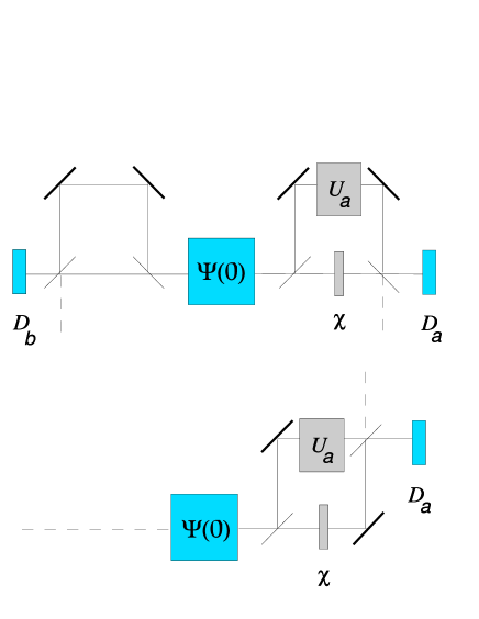
Figure 1: Two-particle interferometry setups to measure phases for internal degrees of freedom in entangled pure state $|\Psi(0)\rangle$. In the upper panel, the pure state phase $\arg\langle\Psi(0)|U_{a}(\tau)\otimes I_{b}|\Psi(0)\rangle$ is measured as a shift in the coincidence interference oscillations obtained at detectors $D_{a}$ and $D_{b}$ by varying the $U(1)$ phase $\chi$. In the lower panel, the mixed state phase $\arg{\text{Tr}}\big{(}\rho_{a}(0)U_{a}(\tau)\big{)}$, with $\rho_{a}(0)={\text{Tr}}_{b}|\Psi(0)\rangle\langle\Psi(0)|$ the mixed input state of subsystem $a$, is similarly measured as a shift at $D_{a}$ by ignoring the subsystem $b$.

It might also be useful to consider the problem from an operational point of view. Let us first consider the two-particle Franson type interferometry setup shown in the upper panel of Fig. 1, with internal pure state $|\Psi(0)\rangle$ affected by $U_{a}(t)\otimes I_{b}$ in the longer arms and by a $U(1)$ shift $\chi$ to one of the shorter arms. To observe the relative phase between $|\Psi(0)\rangle$ and $|\Psi(\tau)\rangle=U_{a}(\tau)\otimes I_{b}|\Psi(0)\rangle$, we require that the source produces particle pairs randomly. Then, if the particles arrive at the two detectors $D_{a}$ and $D_{b}$ simultaneously, they both either took the upper path or the lower path, so that the intensity detected in coincidence at $D_{a}$ and $D_{b}$ becomes Hessmo

$${\cal I}_{ab} \propto \Big{|}e^{i\chi}|\Psi(0)\rangle+|\Psi(\tau)\rangle\Big{|}^{2}$$ (33)

$$= 2+2\Big{|}\langle\Psi(0)|U_{a}(\tau)\otimes I_{b}|\Psi(0)\rangle\Big{|}\cos\Big{[}\chi-\arg\langle\Psi(0)|U_{a}(\tau)\otimes I_{b}|\Psi(0)\rangle\Big{]}.$$

Thus, the relative phase $\arg\langle\Psi(0)|U_{a}(\tau)\otimes I_{b}|\Psi(0)\rangle$ shifts the interference oscillations when $\chi$ varies. To observe the phase of $\rho_{a}(t)={\text{Tr}}_{b}|\Psi(t)\rangle\langle\Psi(t)|$ acquired by subsystem $a$ alone, we instead use the setup shown in the lower panel of Fig. 1 with the same source but where subsystem $b$ is ignored. Here, the output intensity at $D_{a}$ reads Sjoqvistm

$${\cal I}_{a}\propto 2+2\Big{|}{\text{Tr}}\big{(}\rho_{a}(0)U_{a}(\tau)\big{)}\Big{|}\cos\Big{[}\chi-\arg{\text{Tr}}\big{(}\rho_{a}(0)U_{a}(\tau)\big{)}\Big{]}.$$ (34)

Note that ${\text{Tr}}\big{(}\rho_{a}(0)U_{a}(\tau)\big{)}=\langle\Psi(0)|U_{a}(\tau)\otimes I_{b}|\Psi(0)\rangle$ due to the triviality of the evolution of the $b$ subsystem.

Suppose now we first arrange these experiments so that $U_{a}(t)$ yields the pure state parallel transport condition $\langle\Psi(0)|U_{a}^{\dagger}(t)\dot{U}_{a}(t)\otimes I_{b}|\Psi(0)\rangle=0$. In this case, the interference pattern obtained by measuring on both subsystems in coincidence would be shifted by the pure state geometric phase $\gamma_{a}(\tau)$. On other hand, measuring only on subsystem $a$ would yield the same shift, but the interpretation is different: it is the total phase $\alpha_{a}^{M}(\tau)$ acquired by $\rho_{a}(\tau)$, which is in general at variance with $\gamma_{a}^{M}(\tau)$ as this latter phase is based upon the stronger parallel transport conditions. The situation is different when setting up $U_{a}(t)$ so as to parallel transport $\rho_{a}(t)$, i.e., by implementing $U_{a}(t)$ according to Eq. (32). Here, the coincidence and marginal interference pattern are shifted by $\gamma_{a}(\tau)$ and $\gamma_{a}^{M}(\tau)$, respectively, in accordance with the above analysis.

VI Conclusion and Remarks

We have discussed geometric phases of entangled states of bi-partite systems under bi-local unitary evolution and of the mixed states of their subsystems. We conclude:

1. The cyclic geometric phase for entangled states with non-degenerate eigenvalues under bi-local unitary evolution can always be decomposed into a sum of weighted non-modular pure state phases pertaining to the separable components of the Schmidt decomposition, irrespective of forms of local evolution operators, though the same cannot be said for the non-cyclic geometric phase.

2. The mixed state geometric phase of one subsystem is generally different from that of the entangled state even by keeping the other subsystem fixed, though it seems as if the two phases might be same. However, when the evolution operator satisfies the stronger parallel transport conditions for mixed states, the two phases are the same, and the general form of the operators are given.

The difference between geometric phases of bi-partite systems and their parts has its primary cause in entanglement and thus vanishes in the limit of separable states. We hope that the present analysis may trigger multi-particle experiments to test the difference between phases of entangled systems and their subsystems.

References

- (1) M.V. Berry, Proc. R. Soc. London Ser. A 392, 45 (1984).
- (2) B. Simon, Phys. Rev. Lett. 51, 2167 (1983).
- (3) Y. Aharonov and J. Anandan, Phys. Rev. Lett. 58, 1593 (1987).
- (4) J. Anandan and Y. Aharonov, Phys. Rev. D 38, 1863 (1988).
- (5) J. Samuel and R. Bhandari, Phys. Rev. Lett. 60, 2339 (1988).
- (6) N. Mukunda and R. Simon, Ann. Phys. (N.Y.) 228, 205 (1993).
- (7) A.K. Pati, Phys. Lett. A 202, 40 (1995).
- (8) N. Manini and F. Pistolesi, Phys. Rev. Lett. 85, 3067 (2000).
- (9) A. Uhlmann, Rep. Math.Phys. 24, 229 (1986); Lett. Math. Phys.21, 229 (1991).
- (10) E. Sjöqvist, A.K. Pati, A. Ekert, J.S. Anandan, M. Ericsson, D.K.L. Oi, and V. Vedral, Phys. Rev. Lett. 85, 2845 (2000).
- (11) P.B. Slater, Lett. Math. Phys. 60, 123 (2002).
- (12) M. Ericsson, A.K. Pati, E. Sjöqvist, J. Brännlund, and D.K.L. Oi, Phys. Rev. Lett. 91, 090405 (2003).
- (13) K. Singh, D.M. Tong, K. Basu, J.L. Chen, and J.F. Du, Phys. Rev. A 67, 032106 (2003).
- (14) S. Filipp and E. Sjöqvist, Phys. Rev. Lett. 90, 050403 (2003).
- (15) M. Ericsson, E. Sjöqvist, J. Brännlund, D.K.L. Oi, and A.K. Pati, Phys. Rev. A 67, 020101(R) (2003).
- (16) J.F. Du, P. Zou, M. Shi, L.C. Kwek, J.-W. Pan, C.H. Oh, A. Ekert, D.K.L. Oi, and M. Ericsson, Phys. Rev. Lett. 91, 100403 (2003).
- (17) G. Burkard and D. Loss, Phys. Rev. Lett. 88, 047903 (2002); D.P. DiVincenzo, G. Burkard, D. Loss, and E.V. Sukhorukov, in Quantum Mesoscopic Phenomena and Mesoscopic Devices in Microelectronics, edited by I.O. Kulik and R. Ellialtioglu (NATO Advanced Study Institute, Turkey, 1999).
- (18) J.A. Jones, V. Vedral, A. Ekert, and G. Castagnoli, Nature (London) 403, 869 (2000).
- (19) A.K. Ekert, M. Ericsson, P. Hayden, H. Inamori, J.A. Jones, D.K.L. Oi, and V. Vedral, J. Mod. Opt. 47, 2501 (2000).
- (20) X.B. Wang and K. Matsumoto, Phys. Rev. Lett. 87, 097901 (2001).
- (21) E. Sjöqvist, Phys. Rev. A 62, 022109 (2000).
- (22) B. Hessmo and E. Sjöqvist, Phys. Rev. A 62, 062301 (2000).
- (23) D.M. Tong, L.C. Kwek, and C.H. Oh, J. Phys. A 36, 1149 (2003).
- (24) R. Bhandari, Phys. Lett. A 157, 221 (1991); Phys. Lett. A 171, 262 (1992); Phys. Lett. A 171, 267 (1992); Phys. Lett. A 180, 15 (1993).
- (25) R. Bhandari, Phys. Rev. Lett. 89, 268901 (2002); J. Anandan, E. Sjöqvist, A.K. Pati, A. Ekert, M. Ericsson, D.K.L. Oi, and V. Vedral, Phys. Rev. Lett. 89, 268902 (2002).