Rabi spectra - a simple tool for analyzing the limitations of RWA in modelling of the selective population transfer in many-level quantum systems

Abstract

The controlled manipulation of quantum systems is becoming an important technological tool. Rabi oscillations are one of the simplest, yet quite useful mechanisms for achieving such manipulation. However, the validity of simple Rabi theory is limited and its upgrades are usually both technically involved, as well as limited to the simple two-level systems. The aim of this paper is to demonstrate a simple method for analyzing the applicability of the RWA Rabi solutions to the controlled population transfer in complex many-level quantum systems.

I Introduction

State selective manipulation of the discrete-level quantum systems such as atoms, molecules or quantum dots is the ultimate tool for many diverse fields such as laser control of chemical reactions, atom optics, high-precision metrology and quantum computing benetti2000 . The elementary process on which many schemes of such manipulation rely are ’Rabi’ population oscillations between the two selected levels of the system. In the lowest approximation, these oscillations are induced by perturbing the system using coherent monochromatic external drive tuned into resonance with the desired transition. The name of this phenomenon stems from the name of the author of the first approximate analytic assessment of this process rabi1937 .

The original Rabi theory is simple to present and comprehend, but has two drawbacks. The first is that due to the rotating wave approximation (RWA), under which it is obtained, its validity is limited even in pure two-level systems. A number of papers has been published concerning the solution of population dynamics without the RWA shariar2002.1 ; barata2000 ; fujii2003 which are all based on fairly involved mathematical apparatus and hence quite un-intuitive. Also, as these methods are founded on perturbative approaches, the solution in the case of the extreme breakdown of RWA - which is extremely simple (although maybe not very useful) - is seldom mentioned. Secondly, the analytical approach to single-laser Rabi oscillations is generally constrained to simple two level system, and hence its validity is necessarily limited when it is applied to more complex many-level systems. Since many (or, indeed, most…) interesting real systems actually are many-level systems, at least a rough assessment of influence of their structural complexity on the Rabi oscillations between the selected two levels should be done before applying them to complex systems. Finally, looking through the literature I have not managed to find a thorough discussion of the validity of RWA solution for the dynamics of a two level system driven by the perturbation whose frequency is far off resonance.

In this paper all of these questions are addressed. In the first section, mathematically simple yet thorough analysis of the RWA limitations in the two-level systems is presented. In the second, a simple criterium (based on Rabi profiles) for the analysis of the validity of RWA-based solutions is established. This enables a quick estimation of the validity of the Rabi solution for certain system parameters just by visually inspecting the shape of a simple lorenzian curve. Finally, the third section is devoted to discussion of how the concept of Rabi spectrum may be used to estimate the validity of the two-level Rabi solution in a general many-level system.

In all the calculations value of the Planck constant is taken to be $\hbar=1$.

II Rotating wave approximation in a two-level system

In this section a simple, yet thorough analysis of validity of the Rabi RWA solution in the two level system is presented. The results obtained - majority of which are quite well known - will serve as strict mathematical basis for consequent discussions.

II.1 Full dynamical equation

Consider a two-level quantum system. Its dynamics is described by the time dependent Schrödinger equation:

$$i\;\frac{\partial}{\partial t}\psi(\mathbf{x},t)=\left(H_{0}(\mathbf{x})+V(t)\right)\psi(\mathbf{x},t).$$ (1)

$\mathbf{x}$ denotes the set of all spatial coordinates of the system. $H_{0}(\mathbf{x})$ is unperturbed time-independent Hamiltonian of the system, satisfying the eigenequation:

$$H_{0}\;\phi_{i}(\mathbf{x})=E_{i}\;\phi_{i}(\mathbf{x})\ \ ;\ (i=1,2),$$ (2)

where $\phi_{i}(\mathbf{x})$ and $E_{i}$ are eigenfunctions and respective total energies of the unperturbed system. $V(\mathbf{x},t)$ is the homogeneous monochromatic perturbation:

$$V(\mathbf{x},t)=\hat{\mathbf{\sigma}}(\mathbf{x})F_{0}\cos(\omega t).$$ (3)

$\hat{\mathbf{\sigma}}(\mathbf{x})$ is spatial operator odd with respect to central inversion (e.g. dipole, quadrupole, …) through which the perturbation establishes coupling between the two levels of the system. $F_{0}$ is the parameter determining perturbation intensity (which shall be referred to as the perturbation intensity for short). $\omega$ is constant but tunable frequency of the external perturbation. Expressing the solution $\psi(t)$ as an expansion over eigenstates $\phi_{i}(\mathbf{x})$,

$$\psi(t)=\sum_{i=1}^{2}a_{i}(t)\phi_{i}(\mathbf{x})\;e^{-i\omega_{i}t},$$ (4)

Eq. (1) transforms into a system of two coupled differential equations for the time dependent expansion coefficients $a_{i}(t)$:

$$\frac{d}{dt}a_{j}(t)=-iF_{0}\cos(\omega t)\sum_{i=1}^{2}a_{i}(t)I_{ij}e^{-is_{ij}\omega_{ij}t}\ ;(j=1,2).$$ (5)

Here $s_{ij}=-s{ji}\equiv sign(\omega_{ij})$, $\omega_{ij}\equiv|\omega_{i}-\omega_{j}|$  and $I_{ij}\equiv\int\phi_{i}(\mathbf{x})\hat{\mathbf{\sigma}}(\mathbf{x})\phi_{j}(\mathbf{x})d\mathbf{x}$. From the definition it is evident that $I_{12}=I_{21}$ and $I_{11}=I_{22}=0$. Combining the two expansion coefficients into a two-component vector $\bf{a(\tau)}$, expanding a cosine term as $\frac{e^{i\omega t}+e^{-i\omega t}}{2}$ and re-scaling the time variable to

$$\tau\equiv s_{12}\frac{F_{0}I_{12}}{2}t$$ (6)

casts Eq. (5) into convenient matrix form:

$$\frac{d}{d\tau}\bf{a(\tau)}=-i\begin{bmatrix}0&e^{2i\Gamma\tau}+e^{-2i\Delta\tau}\\ e^{-2i\Gamma\tau}+e^{2i\Delta\tau}&0\\ \end{bmatrix}{\bf{a}}(\tau)$$ (7)

where $\Delta\equiv\frac{\omega-\omega_{12}}{F_{0}I_{12}}$ and $\Gamma\equiv\frac{\omega+\omega_{12}}{F_{0}I_{12}}$.

Evolution of the population of a particular level is given by $\Pi_{i}(t)=|a_{i}(\tau)|^{2}$.

II.2 RWA solution and its limitations

The rotating wave approximation hinges on the assumption that the complex exponential terms containing $\Gamma$ in Eq. (7) have only minor (or even negligible) impact on the system dynamics and may hence be dropped in all further calculations. However, in order to fully explore their influence, they shall be keep throughout this calculation.

Now the following procedure is administered: first Eq. (7) is differentiated with respect to $\tau$; then the same equation is used to eliminate $\frac{d\mathbf{a}(\tau)}{d\tau}$ that appears during the differentiation on the right-hand side; finally, the matrix equation is split into two ordinary coupled differential equations for the coefficients $a_{1}(\tau)$ and $a_{2}(\tau)$. The following expression is hence obtained:

$$\frac{d^{2}}{d\tau^{2}}a_{1,2}(\tau) = 2a_{1,2}(\tau)\mp\Delta e^{\mp 2i\Delta\tau}a_{2,1}(\tau)$$

$$\pm \Gamma e^{\pm 2i\Gamma\tau}a_{2,1}(\tau)-2\cos(2(\Gamma+\Delta)\tau)a_{1,2}(\tau)$$

where the first index corresponds to the upper sign and the second to the lower. As no approximations have yet been introduced, this is still the full dynamical equation equivalent to Eq. (7). Initial conditions comprise the whole population of the system located in one of the two levels, with the other level being completely empty.

Keeping only the first term on the right-hand side of Eq. (II.2) leads straight to the on-resonance Rabi RWA solution, sinusoidal population oscillations with period $\Theta_{0}=\pi$ and amplitude $A_{0}=1$ (for details see e.g. demtroeder1988 ). Whether or not the remaining terms on the right-hand side may be considered dynamically insignificant depends on the relation between the period $\Theta_{0}$ and periods of oscillating and complexly rotating parts of these remaining terms. If any of those is much smaller than $\Theta_{0}$ then the value of the elements on the right-hand side in which they are contained averages up to zero during any time interval small compared to the one in which $a_{1}(\tau)$ and $a_{2}(\tau)$ significantly change, and hence they play no dynamical role. Otherwise they have to be taken into consideration.

Shifting the perturbation frequency just slightly away from the resonance, the second term in Eq. (II.2) enters the arena. Taken together, the first two terms lead to the ’generalized’ Rabi oscillations with period $\Theta_{\Delta}=\pi\frac{1}{\sqrt{1+\Delta^{2}}}$ and amplitude $A_{\Delta}=\frac{1}{1+\Delta^{2}}$ (for details see e.g. demtroeder1988 ). So, a shift from the resonance increases the frequency of population oscillations but at the same time reduces their amplitude.

To proceed, note that $\Gamma$ by its definition is always larger than $\Delta$. Indeed, when perturbation is relatively close to the resonance - and if anywhere, the RWA solution should be valid in this spectral region - $\Gamma>>\Delta$. The interplay of the relative dynamical significance of the remaining two terms on the right-hand side in Eq. (II.2) depends only on exact magnitude of $\Gamma$: if $\Gamma>>1$, both of them rotate roughly at the same rate but as the ratio of their amplitudes is $\frac{\Gamma}{2}$, the contribution of the first one overshadows the contribution of the second one; if however, the case is opposite, i.e. $\Gamma<<1$, then the amplitude of the former is so much inferior to that of the later that the contribution of the third term can be neglected when compared to that of the fourth.

Now consider the former case, that is $\Gamma>>1$ so that additional dynamical features that generalized RWA solution fails to encompass are basically provided through the third term in Eq. (II.2). In full numerical solution for this case, these additional features are observed as the additional ’Bloch-Siegert’ oscillations superimposed on the pure sinusoidal population transfer curve. Also, an additional property of the full solution for this case which RWA Rabi solution cannot capture is the shift in the resonant frequency $\omega_{12}$ bloch1940 .

One way to quantify the limitations of the RWA Rabi solution for this case is to try to estimate what the amplitude of these superimposed population oscillations is - as long as they are small enough, RWA solution can be considered as a decent approximation to the full solution. This can be done as follows. The approximate non-RWA solution is sought as a sum $\mathbf{a}_{\Delta}(\tau)+\mathbf{a}_{\Gamma}(\tau)$ where $\mathbf{a}_{\Delta}(\tau)$ is the generalized Rabi RWA solution (taking care of the first two terms in Eq. (II.2)) and $\mathbf{a}_{\Gamma}(\tau)$ the correction due to the additional third term - remember that the fourth term is neglected because of the assumption that $\Gamma>>1$. Inserting this sum into Eq. (7) and assuming that $\mathbf{a}_{\Delta}(\tau)>>\mathbf{a}_{\Gamma}(\tau)$ componentwise, the formal perturbative solution for the correction is obtained:

$$\mathbf{a}_{\Gamma}(\tau)\approx-i\int\begin{bmatrix}0&e^{2i\Gamma\tau}\\ e^{-2i\Gamma\tau}&0\\ \end{bmatrix}\mathbf{a}_{\Delta}(\tau)d\tau.$$ (9)

As $\Gamma>>1$ holds, the frequency $\Theta_{\Delta}$ of $\mathbf{a}_{\Delta}(\tau)$ will certainly be much smaller than the frequency of complex exponentials inside the matrix. Hence, the obtained integral can be evaluated between some $\tau_{0}$ and $\tau$ such that $\tau-\tau_{0}<<\Theta_{\Delta}$ by taking almost constant $\mathbf{a}_{\Delta}(\tau)\approx\mathbf{a}_{\Delta}(\tau_{0})$ outside the integral. The remaining integration is simple and finally yields:

$$\mathbf{a}_{\Gamma}(\tau)\approx\frac{1}{\Gamma}\begin{bmatrix}0&\frac{e^{2i\Gamma\tau}-e^{2i\Gamma\tau_{0}}}{2}\\ \frac{-e^{-2i\Gamma\tau}+e^{-2i\Gamma\tau_{0}}}{2}&0\\ \end{bmatrix}\mathbf{a}_{\Delta}(\tau_{0})$$ (10)

The frequency of the components of $\mathbf{a}_{\Gamma}(\tau)$ is evidently much higher than that of the corresponding components of $\mathbf{a}_{\Delta}(\tau)$. As the amplitude of both matrix elements is $1$, the ratio of amplitudes of the correction components and the generalized Rabi RWA solution components $\frac{|a_{\Gamma\;1,2}(\tau)|}{|a_{\Delta\;1,2}(\tau)|}$ amounts $\frac{1}{\Gamma}$. Thus, while $\Gamma>>1$, $\mathbf{a}_{\Delta}(\tau)>>\mathbf{a}_{\Gamma}(\tau)$ the RWA generalized Rabi solution is a good approximation to the full solution and the dynamical significance of the third term in Eq. (II.2) may be neglected.

The last remaining term in Eq. (II.2) has a fixed amplitude equal to $4$. It can be neglected if $\Gamma+\Delta>>1$, due to the zero-averaging effect of its rapid rotation, and since $\Delta$ can be reduced to zero, in the worst case this reduces to $\Gamma>>1$ - which is the same as for the third component. However, this term has a prominent role in the extreme situation, when $\Gamma<<1$. In such a case, the third term may be neglected due to its vanishing amplitude, and since $\Delta<\Gamma$ even more so may the second term. Eq. (II.2) then reduces to:

$$\frac{d^{2}}{d\tau^{2}}a_{1,2}(\tau)=-2\Bigl{(}1+\cos(2(\Gamma+\Delta)\tau)\Bigr{)}a_{1,2}(\tau)$$ (11)

which leads to the population oscillations with amplitude $1$, but with temporally modulated period $\Theta(\tau)\approx\pi\frac{1}{|1+\cos(2(\Delta+\Gamma)\tau)|}$. As with the third term, this one is also inherently related to the inclusion of the ’non-RWA’ contributions in matrix in Eq. (7). It should be kept in mind that in this case the perturbation is extremely strong. Under such circumstances the corresponding potential $V(t)$ in dynamical equation (Eq. (3)) might need to be corrected with higher order interaction terms (quadrupole, octupole,…). Indeed, it may also happen that the structure of the original two-level system becomes significantly distorted or even that the system breaks up completely. Hence this result might not be very useful from the point of controlled system manipulation.

All in all, it may be concluded that the Rabi RWA solution is an excellent approximation to the exact solution of Eq.(7) in complete spectral range $0<\omega<\infty$ of perturbation frequencies - and not just close to resonance $\omega_{12}$ - as long as:

$$\Gamma>>1.$$ (12)

III Rabi profile analysis

In this section the notion of Rabi profile is introduced and it is demonstrated how the obtained condition for the validity of the Rabi RWA solution, $\Gamma>>1$, can conveniently be visualized in terms of it.

III.1 Rabi profile of a single system transition

Rabi profile of the transition between levels 1 and 2 simply refers to the amplitude of population oscillations exhibited by the generalized Rabi RWA solution, considered as a function of the driving frequency $\omega$. It is parameterized with the total coupling strength (or coupling), $D_{12}\equiv F_{0}I_{12}$ and the resonant frequency of the system, $\omega_{12}$:

$$P_{12}(\omega)=\frac{1}{1+\frac{(\omega-\omega_{12})^{2}}{(D_{12})^{2}}}$$ (13)

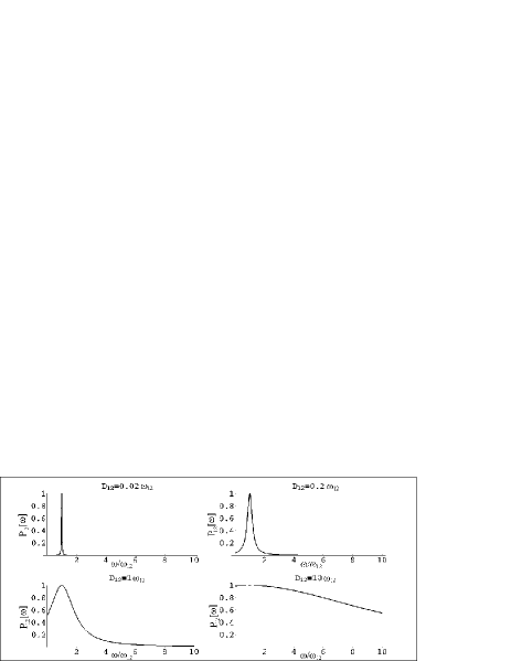
Figure 1: Rabi profiles of a single spectral line. In each graph, respective coupling $D_{12}$ is indicated above the graph. Observe how the profile’s half-width increases with increasing coupling. The corresponding dynamics of a two-level system driven by the resonant perturbation is given in Fig.2. On the abscissa, perturbation frequency $\omega$ is given in the units of the resonant frequency $\omega_{12}$ of the system.

As can be seen from the Fig. 1, it is a simple bell-shaped curve centered on $\omega_{12}$ with the half-width at half-maximum (or halfwidth) equal to $D_{12}$.

Expressing the condition (12) in terms of the drive frequency, the resonant transition frequency and the coupling, a simple criterium for estimating the validity of the generalized Rabi RWA solution in the particular two-level system driven by the external homogenous coherent perturbation is obtained: $D_{12}<<\omega_{12}+\omega$. In the worst case this reduces to:

$$D_{12}<<\omega_{12}$$ (14)

or, put in words, distance of the profile’s center from the origin of the spectrum ($\omega=0$) must be much greater than the profile’s half-width. We may also rephrase it as: ’At the origin of the spectrum the height of the profile must be negligible’. If this condition is fulfilled, population of a two-level system driven with any desired frequency $\omega$ will exhibit pure sinusoidal oscillations with amplitude equal to the height $P_{12}(\omega)$ of the Rabi profile at the selected frequency and period equal to:

$$T_{12}(\omega)=\frac{\pi}{|D_{12}|}\sqrt{P_{12}(\omega)}$$ (15)

Fig. 2 exhibits four cases of the population dynamics in a resonantly driven two-level system. These are obtained as the ’exact’ numerical solution to Eq. (7) (using the NDSolve method from MATHEMATICA software package). The four presented cases respectively correspond to Rabi profiles in Fig. 1, as indicated with the value of coupling $D_{12}$ above each graph. In the first case, the coupling is relatively weak so that the condition (12) is fully satisfied (actually, $\Gamma=50$) and the pure sinusoidal population oscillations are observed. The second case is a limiting one ($\Gamma=5$): a minor rapidly oscillating Bloch-Siegert component may be observed superimposed on top of major sinusoidal oscillations. In the third case $\Gamma=1$ so that the major discrepancy from the sinusoidal oscillations is expected, and is indeed observed, with the Bloch-Siegert and the Rabi components being roughly of the same order of magnitude. The last case ($\Gamma=0.1$) corresponds to lower limit of the extreme coupling ($\Gamma<<1$), and as predicted, the quasi-sinusoidal oscillations with time-dependent period are observed.

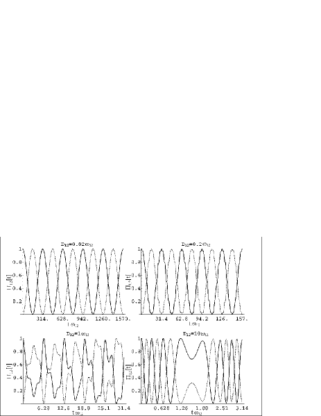
Figure 2: The exact numerical solution for the population dynamics of the two-level system subjected to a resonant perturbation. The quantity on the abscissa is time expressed through dimensionless variable $t\omega_{12}$, and the ordinate is $\Pi_{1,2}(t)$. Initially the complete population is located in level 1. Populations $\Pi_{1}(t)$ and $\Pi_{2}(t)$ are respectively represented with a full and a dotted line. Tick-marks are located at integral multiples of the population transfer period, calculated from Eq. (15) corresponding to the respective value of $D_{12}$.

Fig. 3 displays the numerical solutions for the population dynamics of a two-level system driven by the off-resonant perturbation. The Rabi profile (displayed in the top graph) is common for all four cases, with the coupling equal to $D_{12}=0.05\omega_{12}$. By visual inspection it may be checked that the condition for validity of the Rabi RWA solution is fulfilled, while analytically it amounts to $\Gamma\geq 20$. The four perturbation frequencies ($\omega_{\mathbf{a}}=1.050\omega_{12}$, $\omega_{\mathbf{b}}=0.850\omega_{12}$, $\omega_{\mathbf{c}}=0.503\omega_{12}$ and $\omega_{\mathbf{d}}=2.580\omega_{12}$) are chosen so that $P_{12}(\omega_{\mathbf{a}})=0.5$, $P_{12}(\omega_{\mathbf{b}})=0.1$, $P_{12}(\omega_{\mathbf{c}})=0.01$ and $P_{12}(\omega_{\mathbf{d}})=0.001$. Vertical gridlines in bottom four graphs are drawn at integral multiples of the predicted population oscillation time, determined from (15). Horizontal gridlines are drawn at the predicted Rabi RWA value of the population oscillation amplitude determined from (13). In the case a. the observed dynamics is clearly sinusoidal oscillations with the predicted amplitude and period. In the case b. the excellent agreement between the predicted Rabi RWA values and the numerical results is also clear. However, the minor Bloch-Siegert oscillations of amplitude $\frac{1}{\Gamma}\approx 0.05$ may be noted. In the case c. again the predictions are quite fair, although the amplitude of the Bloch-Siegert oscillations is now of the same order as the Rabi component so the dynamics is not purely sinusoidal, but is rather doubly periodic. In the last case, d. situation is similar to the one in the case c., but as $\Gamma$ is somewhat larger for this case, the agreement is somewhat better. Altogether, the usefulness of the graphical criterium is clear. With narrower profiles situation is even better.

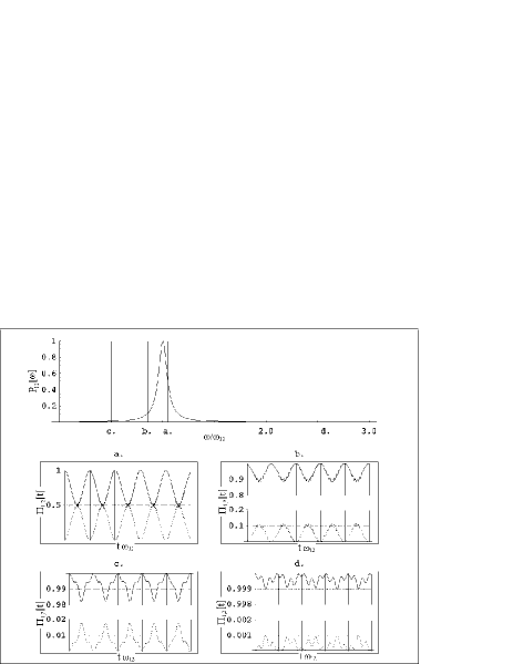
Figure 3: Numerical solutions for the population dynamics of a two-level system subjected to non-resonant perturbations. On the top graph the common Rabi profile is displayed. Vertical lines indicate different perturbation frequencies for each of the four cases presented. Letters under the lines indicate which dynamics graph corresponds to each perturbation. On the four bottom graphs the corresponding population dynamics is displayed. Horizontal lines indicate the expected value of amplitude of population oscillations determined according to the corresponding height of the Rabi profile (Eq. (13)) in each particular case. Vertical lines mark the multiples of the oscillation period determined from Eq. (15). The excellent agreement of these two approximate expressions obtained within the RWA, and the ’actual’ behavior represented by the numerical solution is quite clear.

III.2 Many-level system and the Rabi spectrum

As a first instance of many-level system a three-level one shall be considered. It is actually the most important example, as all the consequent conclusions on the behavior of the many-level systems are a mere generalization of the findings from a three-level case. Let the internal structure of this system be such that the drive couples level 1 to level 2 with the total strength $D_{12}\equiv F_{0}I_{12}$ and level 2 to level 3 with the total strength $D_{23}\equiv F_{0}I_{23}$, but does not couple level 1 directly to level 3 (i.e. $I_{13}=0$). The spectrum of the system hence contains two resonant frequencies, $\omega_{12}$ and $\omega_{23}$. Initially let the whole population be located in level 2. The main goal is to transfer it to the level 1 minimizing both the transfer time and the loses to the level 3. Based on the results discussed in the previous section the dynamics of the three-level system might be predicted to some extent by inspecting the common plot of the two Rabi profiles $P_{12}(\omega)$ and $P_{23}(\omega)$ (top graphs in Fig. 4, 5 and 6). Such a plot containing all the Rabi profiles of the spectral lines which couple any of the two targeted levels (1 and 2 in this case) among themselves and to the rest of the system (just level 3 in this case) shall be referred to as the Rabi spectrum of the particular targeted transition.

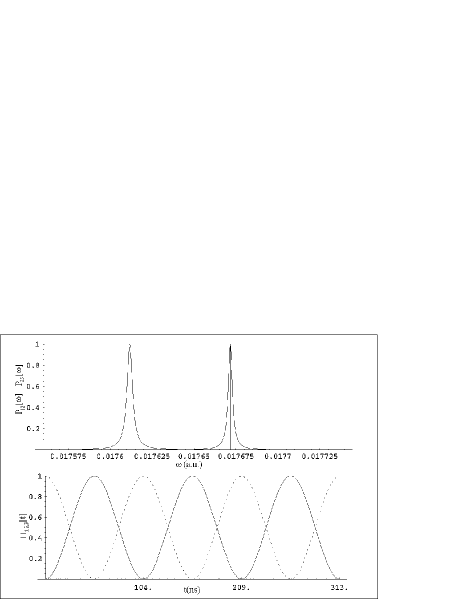
Figure 4: Rabi spectrum and the numerical solution for the population dynamics of a three-level system. On the top graph the two Rabi profiles corresponding to the two resonant lines of the system are plotted alongside. The two spectral lines roughly correspond to the two of the low-laying ro-vibrational transitions in the HF molecule. The abscissa is $\omega$ (atomic units) and the ordinate is $P_{12,23}(\omega)$ (dimensionless). Perturbation frequency is indicated with the vertical line on the Rabi spectrum plot, and it is set to the resonant frequency $\omega_{12}$. The bottom graph presents the population dynamics of all three populations. The full line is $\Pi_{1}(t)$, the dashed line is $\Pi_{2}(t)$. The population of level 3 would be drawn as the dotted line, but it is so negligibly small at all times that it cannot be distinguished from the x-axis.

Assume that both profiles are ’narrow’ so that for both of them Eq. (14) holds. Further assume that both profiles are also ’narrower’ then the distance between their centers, $|\omega_{12}-\omega_{23}|>>D_{12},D_{23}$. This situation is displayed on top graph in Fig. 4, and it can always be achieved by sufficiently reducing the drive intensity, $F_{0}$. Now consider each of the two transitions separately. Consider tuning the perturbation to $\omega_{12}$. As $P_{12}(\omega_{12})=1$ and $P_{23}(\omega_{12})<<1$, such perturbation would induce the complete population transfer oscillations on transition $1\leftrightarrow 2$ and almost negligible population oscillations on transition $2\leftrightarrow 3$. Hence, if such a drive is applied to the three-level system, it might be expect that it would indeed produce complete population oscillations between levels 1 and 2 and would have almost negligible effect on level 3. Validity of this prediction can be clearly observed by inspecting the numerical solution presented in the bottom graph of Fig. 4.

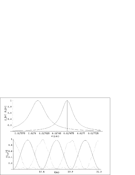
Figure 5: Rabi spectrum and the numerical solution for the population dynamics of a three-level system. On the top graph the two Rabi profiles corresponding to the two resonant lines of the system are plotted alongside. The two spectral lines roughly correspond to the two of the low-laying ro-vibrational transitions in the HF molecule. The abscissa is $\omega$ (atomic units) and the ordinate is $P_{12,23}(\omega)$ (no units). The perturbation frequency is indicated with the vertical line on the Rabi spectrum plot, and it is set to the resonant frequency $\omega_{12}$. The bottom graph presents the population dynamics of all three populations. The full line is $\Pi_{1}(t)$, the dashed line is $\Pi_{2}(t)$ and the dotted line is $\Pi_{3}(t)$.

According to Eq. (15), an increase in the speed of population transfer can be achieved by increasing the coupling through increasing the perturbation intensity $F_{0}$. Suppose that system parameters (resonant frequencies and coupling integrals) are such that after the drive intensity is increased both profiles still satisfy Eq. (14), but that now the profile of the undesired transition 2-3 broadens to such an extent that $P_{23}(\omega_{12})$ is still small but not negligible any more. This situation is displayed on the top graph of the Fig. 5. Considering again each transition by itself, drive with frequency $\omega_{12}$ would again produce the complete periodic population transfer on transition $1\leftrightarrow 2$, but would also produce a clearly observable - albeit not complete - population oscillations on $2\leftrightarrow 3$. So in the three level system we expect the population dynamics would change from that in the previous case as now both transitions ’react’ significantly to the applied drive. Based on the discussion in the previous section, it can be suggested that it would roughly comprise of most population being exchanged along transition $1\leftrightarrow 2$ with the remaining fraction being now also exchanged among levels 2 and 3. This is clearly observed from the numerical solution displayed on the bottom graph of Fig. 5. It can also be observed that the maximum amplitude of the perturbing level’s population equals almost exactly $P_{23}(\omega_{12})$.

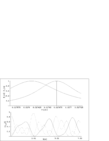
Figure 6: Rabi spectrum and the numerical solution for the population dynamics of a three-level system. On the top graph the two Rabi profiles corresponding to the two resonant lines of the system are plotted alongside. The two spectral lines roughly correspond to the two of the low-laying ro-vibrational transitions in the HF molecule. The abscissa is $\omega$ (atomic units) and the ordinate is $P_{12,23}(\omega)$ (no units). The perturbation frequency is indicated with the vertical line on the Rabi spectrum plot, and it is set to the resonant frequency $\omega_{12}$. The bottom graph presents the population dynamics of all three populations. The full line is $\Pi_{1}(t)$, the dashed line is $\Pi_{2}(t)$ and the dotted line is $\Pi_{3}(t)$.

By further increasing the perturbation intensity (Fig. 6), a simple sinusoidal pattern of oscillations on the transition $1\leftrightarrow 2$ disappears completely. Hence the perturbation this strong cannot be employed to drive the efficient population transfer along the transition $1\leftrightarrow 2$. This suggests that in a general many-level quantum system there is an upper limit to speed of the efficient population transfer (i.e. such that the great majority of the population is transferred) along each particular transition. This limit is determined exclusively by the internal properties of the system. Consider two levels $\alpha$ and $\beta$ of a many-level system that are directly coupled by the applied drive, i.e. such that $I_{\alpha\beta}\neq 0$. The efficient transfer along the transition $\alpha\leftrightarrow\beta$ is feasible as long as none of the profiles from that particular transition’s Rabi spectrum has significant height at the resonant frequency of that transition - except, of course, the Rabi profile of that selected transition (which is 1 at its own resonant frequency). Certainly, it should also be kept in mind that the Rabi profile of that selected transition has to have negligible height at the origin, i.e. it has to satisfy the condition (12) for the validity of pure RWA solution at that transition.

IV Conclusion

The most important result of this paper is the establishment of the simple graphical criterium for the validity of the approximate two-level RWA solution in modelling the population transfer in a general many-level discrete quantum mechanical system. The first hint of Rabi spectrum method that I am aware of appeared quite some time ago quack1985 - Fig. 5 in that paper is actually the Rabi spectrum plot. Looking at Fig. 6b in the same paper, minor oscillations can be noticed superimposed on top of almost pure Rabi oscillations of one of the populations. These minor oscillations gave me the idea that Rabi profile plots might be used as an indicator as to when the pure Rabi oscillations, which are a straightforward two-level RWA solution, fail to provide the satisfactory solution to the complete dynamics of a more complex many-level system.

Although the presented analysis is mathematically quite simple, it nevertheless enables a very good order-of-magnitude estimates for maximum driving field intensities that can be used to efficiently drive the selected transition. Rabi spectra method hence hints on one interesting application. Namely, knowing the details of the internal structure of a particular quantum system, the Rabi spectrum for each transition in that system can be calculated. This data can then be used to quickly quantitatively estimate the lower limit for clean population transfer time that can be achieved on any particular transition. Finally, a numerical scheme can be build to search for the quickest pathway through the system along which population can be transferred between any two selected levels, and lower limit of the time needed can be estimated.

Most of all, Rabi spectra method offers conceptual simplicity and intuitiveness which are both of utmost importance when whole subject is presented either to interested non-experts or to newcomers in the field. Hence it can be considered very suitable both as a quick lab-reference tool as well as a simple didactic introduction into much more involved strict quantitative theory.

The full analytical treatment of the selective population transfer mechanism provides many additional interesting results. It can thus be shown bonacci2003.2 that by using analytically determined chirp (i.e. time dependent variation of the perturbation frequency) instead of resonant frequency to drive any particular transition, more efficient population transfer can be achieved.

References

- (1) C. Benetti, D. DiVincenzo, Quantum information and computation, Nature 404 (6775) (2000) 247–255.
- (2) I. Rabi, Space quantization in a gyrating magnetic field, Phys. Rev. 51 (8) (1937) 652–654.
- (3) M. Shariar, P. Pradhan, Fundamental limitation on qubit operations due to the Bloch-Siegert oscillation (quant-ph/0212121).
- (4) J. Barata, W. Wreszinski, Strong coupling theory of two level atoms in periodic fields, Phys.Rev.Lett. 84 (10) (2000) 2112–2115 (quant-ph/9906029).
- (5) K. Fujii, Two-level system and some approximate solutions in the strong coupling regime (quant-ph/0301145).
- (6) W. Demtroeder, Laser spectrocopy: basic concepts and instrumentation, 1st Edition, Springer-Verlag, Berlin, 1988.
- (7) F. Bloch, A. Siegert, Magnetic resonance for nonrotating fields, Phys.Rev. 57 (6) (1940) 522.
- (8) M. Quack, E. Sutcliffe, Primary photophysical processes in IR multiphoton excitation: wavepacket motion and state selectivity, Infrared Physics 25 (1-2) (1985) 163–173.
- (9) D. Bonacci, Analytic pulse design for selective population transfer in many-level quantum systems: maximizing the amplitude of population oscillations, accepted for publication in Phys.Rev.A (quant-ph/0310034).