Abstract

The design of efficient quantum circuits is an important issue in quantum computing. It is in general a formidable task to find a highly optimized quantum circuit for a given unitary matrix. We propose a quantum circuit design method that has the following unique feature: It allows to construct efficient quantum circuits in a systematic way by reusing and combining a set of highly optimized quantum circuits. Specifically, the method realizes a quantum circuit for a given unitary matrix by implementing a linear combination of representing matrices of a group, which have known fast quantum circuits. We motivate and illustrate this method by deriving extremely efficient quantum circuits for the discrete Hartley transform and for the fractional Fourier transforms. The sound mathematical basis of this design method allows to give meaningful and natural interpretations of the resulting circuits. We demonstrate this aspect by giving a natural interpretation of known teleportation circuits.

Keywords: Quantum circuits, quantum signal transforms, unitary error bases, circulant matrices, teleportation.

1 Introduction

The worldwide efforts to build a viable quantum computer have one source of motivation in common: The potential to solve certain problems faster on a quantum computer than on any classical computer. There are a number of ways to specify quantum algorithms but the formulation of quantum algorithms as a uniform family of quantum circuits is the most popular choice.

Deriving an efficient quantum circuit for a given unitary matrix is a daunting, and, frustratingly, often impossible, task. There exist a small number of efficient quantum circuits, and even fewer quantum circuit design methods. If efficient quantum circuits are rare and difficult to derive, then is only natural to try to reuse these quantum circuits in the construction of other quantum circuits. We present in this paper a new design principle for quantum circuits that is exactly based on this idea.

Suppose that we want to realize a given unitary matrix $A$ as a quantum circuit. Suppose that we know a number of quantum circuits realizing unitary matrices $D(g)$ of the same size as $A$. We choose a small subset of these unitary matrices such that the algebra generated by the matrices $D(g)$ contains $A$. Roughly speaking, if the generated algebra has some structure, e.g. is a finite dimensional (twisted) group algebra, then we are able to write down a quantum circuit realizing $A$, which reuses the implementations of the matrices $D(g)$.

As a motivating example serves the discrete Hartley transformation, which is a variant of the discrete Fourier transform defined over the real numbers. In Section 3, we show how the Hartley transforms can be realized by combining quantum circuits for the discrete Fourier transform and its inverse. We generalize the idea behind this construction in the subsequent sections.

An essential ingredient of our method are circulant matrices and certain block-diagonal matrices, which are introduced in Sections 4 and 5. In Section 6 we present the main result of this paper. We show how to derive a quantum circuit for a unitary matrix $A$, which can be expressed as a linear combination $U=\alpha_{1}D(g_{1})+\ldots+\alpha_{n}D(g_{n})$ of unitary matrices $D(g_{i})$ with known quantum circuits. For ease of exposition, we do not state the theorem in full generality; the generalizations of the method are discussed in Sections 7 and 8.

There is a relation between Kitaev’s method for eigenvalue estimation of unitary operations and the present method which is explored in Section 9. Section 10 demonstrate the design principle with the help of some simple examples. We revisit the Hartley transform in Section 10.1, and discuss fractional Fourier transforms in Section 10.2. We give an interpretation of the well-known teleportation circuit in terms of projective circulants in Section 10.3.

Notations. We denote by ${\mathbb{Z}}$, ${\mathbb{Z}}/n{\mathbb{Z}}$, ${\mathbb{R}}$, and ${\mathbb{C}}$ the ring of integers, the ring of integers modulo $n$, the field of real numbers, and the field of complex numbers, respectively. The group of unitary $n\times n$ matrices is denoted by ${\cal U}(n)$. We denote the identity matrix in ${\cal U}(n)$ by $\mbox{\bf 1}_{n}$.

2 Background

We consider quantum computations that manipulate the state of $n$ two-level systems. A two-level system has two clearly distinguishable states $\left|0\right>$ and $\left|1\right>$, which are used to represent a bit. We refer to such a two-level system as a quantum bit, or shortly a qubit. The state of $n$ quantum bits is mathematically represented by a vector in ${\mathbb{C}}^{2^{n}}$ of norm 1. We choose a distinguished orthonormal basis of ${\mathbb{C}}^{2^{n}}$ and denote its basis vectors by $\left|x_{n-1},\dots,x_{0}\right>$, where $x_{i}\in\{0,1\}$ with $0\leq i<n$.

A quantum gate on $n$ qubits is an element of the group of unitary matrices ${\cal U}(2^{n})$. We will use single-qubit gates and controlled-not gates. A single-qubit gate acting on qubit $i$ is given by a matrix of the form $U^{(i)}=\mbox{\bf 1}_{2^{n-i-1}}\otimes U\otimes\mbox{\bf 1}_{2^{i}},$ with $U\in{\cal U}(2)$. A controlled-not gate with control qubit $i$ and target qubit $j$ is defined by

$$\left|x_{n-1},\dots,x_{j+1},x_{j},x_{j-1},\dots,x_{0}\right>\mapsto\left|x_{n-1},\dots,x_{j+1},x_{i}\oplus x_{j},x_{j-1},\dots,x_{0}\right>,$$

where $\oplus$ denotes addition modulo 2. We denote this gate by ${\rm CNOT}^{(i,j)}$. We will refer to single-qubit gates and controlled-not gates as elementary gates.

It is well-known [1] that the single-qubit gates and the controlled-not gates are universal, meaning the set

$${\cal G}=\{U^{(i)},{\rm CNOT}^{(i,j)}\mid U\in{\cal U}(2),\ i,j\in\{1,\dots,n\},\ i\neq j\}$$

generates the unitary group ${\cal U}(2^{n})$. In other words, each matrix $U\in{\cal U}(2^{n})$ can be expressed in the form $U=w_{1}w_{2}\ldots w_{k}$ with $w_{i}\in{\cal G}$, $0\leq i<k$. Of special interest are the shortest possible words for $U$. We denote by $\kappa(U)$ the smallest $k$ such that there exists a word $w_{1}w_{2}\cdots w_{k}$, with $w_{i}\in{\cal G}$, $0\leq i<k$, such that $U=w_{1}w_{2}\ldots w_{k}$.

The complexity measure $\kappa$ turns out to be rather rigid. It is desirable to allow a variation which gives additional freedom. We say that a unitary matrix $V$ realizes $U$ with the help of ancillae provided that $V$ maps $\left|0\right>\otimes\left|x\right>\mapsto\left|0\right>\otimes U\left|x\right>$ for all $\left|x\right>\in{\mathbb{C}}^{2^{n}}$. We define $\kappa_{{\rm anc}}(U)$ to be the minimum $\kappa(V)$ of all unitary matrices $V$ realizing $U$ with the help of ancillae.

As examples, we mention the following bounds on the complexity for well-known transforms acting on $n$ quantum bits: the Hadamard transform $\kappa(H_{2}^{\otimes n})=O(n)$; the discrete Fourier transform $\kappa(F_{2^{n}})=O(n^{2})$ when realized without ancillae [2, 3], and $\kappa_{{\rm anc}}(F_{2^{n}})=O(n(\log n)^{2}\log\log n)$ when realized with ancillae [4]. Various unitary signal transformations with fast quantum realizations can be found in [5, 6, 7, 8, 9].

3 A Motivating Example

Assume that we have already found an efficient quantum circuit for a given unitary matrix $U\in{\cal U}(2^{n})$ with $O(n^{c})$ quantum gates, $c$ some constant. We would like to find an efficient quantum circuit for a polynomial function $f(U)$ of $U$, allowing ancillae qubits. If we succeed, then this would prove that $\kappa_{\rm anc}(f(U))\in O(n^{k})$ for some constant $k\geq 0$.

As an example, consider the discrete Hartley transform $A_{N}\in{\cal U}(N)$ of length $N\in{\mathbb{N}}$, which is defined by

$$A_{N}:=\frac{1}{\sqrt{N}}\Big{[}{\rm cas}\Big{(}\frac{2\pi kl}{N}\Big{)}\Big{]}_{k,l=0,\ldots,N-1},$$

where the function ${\rm cas}:{\mathbb{R}}\rightarrow{\mathbb{R}}$ is defined by ${\rm cas}(x):=\cos(x)+\sin(x)$. The discrete Hartley transform is well-known in classical signal processing, cf. [10, 11]. If we denote the discrete Fourier transform by $F_{N}$, then

$$A_{N}=\left(\frac{1-i}{2}\right)\;F_{N}+\left(\frac{1+i}{2}\right)\;F_{N}^{3}$$

is an immediate consequence of the definitions.

Let $N=2^{n}$. We will now derive an efficient quantum circuit implementing the Hartley transform $A_{N}$ with one auxiliary quantum bit.

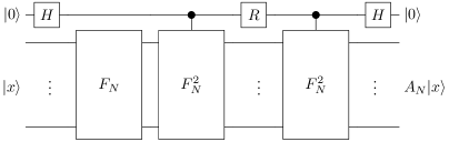
Figure 1: Circuit realizing a quantum Hartley transform

Lemma 1

The discrete Hartley transform can be realized by the circuit shown in Figure 1, where $R$ denotes the unitary circulant matrix

$$R:=\frac{1}{2}\left(\begin{array}[]{rr}1-i&1+i\\ 1+i&1-i\end{array}\right)$$

and $H$ the Hadamard transform.

Proof. Let $\widehat{F}_{N}=\Lambda_{1}(F_{N})$ denote the unitary matrix effecting a discrete Fourier transform on the $n$ least significant bits if the most significant (ancilla) bit is set; in terms of matrices $\hat{F}_{N}=\mbox{\bf 1}_{N}\oplus F_{N}$. Similarly, let $\widehat{F}_{N}^{2}=\mbox{\bf 1}_{N}\oplus F_{N}^{2}$.

We now show that the circuit shown in Figure 1 computes the linear transformation $\left|0\right>\left|x\right>\mapsto\left|0\right>A_{N}\left|x\right>$ for all vectors $\left|x\right>\in{\mathbb{C}}^{n}$ of unit length. Proceeding from left to right in the circuit, we obtain

$$\left|0\right>\left|x\right> \stackrel{{\scriptstyle H}}{{\longmapsto}} \frac{1}{\sqrt{2}}(\left|0\right>+\left|1\right>)\left|x\right>$$

$$\stackrel{{\scriptstyle F_{N}}}{{\longmapsto}} \frac{1}{\sqrt{2}}(\left|0\right>+\left|1\right>)F_{N}\left|x\right>$$

$$\stackrel{{\scriptstyle\widehat{F}_{N}^{2}}}{{\longmapsto}} \frac{1}{\sqrt{2}}\left|0\right>F_{N}\left|x\right>+\frac{1}{\sqrt{2}}\left|1\right>F_{N}^{3}\left|x\right>$$

$$\stackrel{{\scriptstyle R}}{{\longmapsto}} \frac{1}{\sqrt{2}}\left|0\right>\left(\frac{1}{2}(1-i)F_{N}+\frac{1}{2}(1+i)F_{N}^{3}\right)\left|x\right>$$

$$+\frac{1}{\sqrt{2}}\left|1\right>\left(\frac{1}{2}(1+i)F_{N}+\frac{1}{2}(1-i)F_{N}^{3}\right)\left|x\right>$$

$$= \frac{1}{\sqrt{2}}\left|0\right>A_{N}\left|x\right>+\frac{1}{\sqrt{2}}\left|1\right>F_{N}^{-2}A_{N}\left|x\right>$$

$$\stackrel{{\scriptstyle\widehat{F}_{N}^{2}}}{{\longmapsto}} \frac{1}{\sqrt{2}}(\left|0\right>+\left|1\right>)A_{N}\left|x\right>$$

$$\stackrel{{\scriptstyle H}}{{\longmapsto}} \left|0\right>A_{N}\left|x\right>$$

as desired. Note that we have used the property that the discrete Fourier transform has order four, i. e., $F_{N}^{4}=\mbox{\bf 1}$. $\Box$

We cast this factorization and the corresponding complexity cost in terms of elementary quantum gates in the following theorem.

Theorem 1

The discrete Hartley transform $A_{2^{n}}\in{\cal U}(2^{n})$ can be implemented with $O(n(\log n)^{2}\log\log n)$ quantum gates on a quantum computer.

Proof. Recall that the discrete Fourier transform $F_{2^{n}}$ can be implemented with $O(n(\log n)^{2}\log\log n)$ quantum gates, see [4]. The claim is an immediate consequence of Lemma 1.  $\Box$

We pause here to discuss some noteworthy features of the preceding example. We notice that the discrete Fourier transform $F_{2^{n}}$ satisfies the relation $F_{2^{n}}^{4}=1$, and that all powers $\mbox{\bf 1}_{2^{n}},F_{2^{n}},F_{2^{n}}^{2},F_{2^{n}}^{3}$ have fast implementations with known quantum circuits. We constructed the Hartley transform as a linear combination of some of those powers, namely as a linear combination of $F_{2^{n}}$ and $F_{2^{n}}^{3}$ using the circuit shown in Figure 1. A nice feature of this circuit is that any improvement in the design of quantum algorithms for the discrete Fourier transform will directly lead to an improved performance of the discrete Hartley transform, since the circuits for the discrete Fourier transform a simply reused in the Hartley transform circuit.

We will generalize this idea in the following sections. The methods are much more general. We will even be able to combine several different circuits, assuming that some regularity conditions are satisfied. The factorization of the Hartley transform implied by Lemma 1 will be obtained as a special case of this more general theory in Section 10.1.

4 Circulant Matrices

Our goal is to derive a circuit implementing linear combinations of matrices. This is not an easy task, because all operations need to be unitary. We assume that the algebra generated by the matrices has some structure which we can exploit when deriving the circuit. Our approach will be particularly successful when the generated algebra $\mathcal{A}$ is a finite dimensional (twisted) group algebra. In this case, we can write down a single generic circuit which is able to implement any unitary matrix $U$ contained in $\mathcal{A}$. In the case of a group algebra, a group-circulant determines which matrix $U$ is implemented by the generic circuit.

Recall the definition of a group-circulant [12, 13]:

Definition 1

Let $G$ be a finite group of order $d$. Choose an ordering $(g_{1},\ldots,g_{d})$ of the elements of $G$ and identify the standard basis of ${\mathbb{C}}^{d}$ with the group elements of $G$. Let $\left|c\right>=\sum_{g\in G}c_{g}\left|g\right>\in{{\mathbb{C}}}^{d}$ denote a vector indexed by the elements of $G$. Then the $d\times d$-matrix

$${\rm circ}_{G}(\left|c\right>):=(c_{g^{-1}h})_{g,h\in G}$$ (1)

is a group-circulant for the group $G$.

The following example covers the important special case of cyclic circulants.

Example 2

Let $G={{\mathbb{Z}}}_{d}$ be the cyclic group of order $d$ generated by $x$ and the elements of $G$ ordered according to $(1,x,x^{2},\ldots,x^{d-1})$. The circulant corresponding to $\left|c\right>:=\sum_{i=0}^{d-1}c_{i}\left|x^{i}\right>\in{{\mathbb{C}}}^{d}$ takes the form

$$\left(\begin{array}[]{cccc}c_{0}&\cdots&c_{d-2}&c_{d-1}\\ c_{d-1}&\cdots&c_{d-3}&c_{d-2}\\ \vdots&\ddots&\ddots&\vdots\\ c_{1}&\cdots&c_{d-1}&c_{0}\end{array}\right).$$

We see that each row is obtained from the previous one by a cyclic shift to the right.

The following crucial observation connects group-circulants with the coefficients $\alpha_{g}$ in linear combinations. The linear independence of the representing matrices $D(g)$ of a finite group $G$ ensures that the circulant $(\alpha_{g^{-1}h})_{g,h\in G}$ is a unitary matrix.

Key Lemma 3

Let $n$ be a positive integer. Let $\{D(g):g\in G\}$ be a set of linearly independent unitary matrices which form a finite subgroup of ${\cal U}(n)$. Furthermore, let $A\in{\cal U}(n)$ be a linear combination of the matrices $D(g)$,

$$A=\sum_{g\in G}\alpha_{g}D(g),$$

with certain coefficients $\alpha_{g}\in{\mathbb{C}}$. Then the associated group circulant matrix $C_{A}:=(\alpha_{g^{-1}h})_{g,h\in G}$ is unitary.

Proof. Multiplying $A$ with $A^{\dagger}$ yields

$$A\cdot A^{\dagger} = \Big{(}\sum_{g\in G}\alpha_{g}D(g)\Big{)}\cdot\Big{(}\sum_{h\in G}\overline{\alpha_{h}}D(h)^{\dagger}\Big{)}$$

$$= \sum_{g\in G}\sum_{h\in G}\alpha_{g}\overline{\alpha_{h}}D(g)D(h)^{\dagger}$$

$$= \sum_{g\in G}\Big{(}\sum_{h\in G}\alpha_{gh}\overline{\alpha_{h}}\Big{)}D(g).$$

Since the matrices $D(g)$ are linearly independent, it is possible to compare coefficients with $A\cdot A^{\dagger}=\mbox{\bf 1}_{n}$, which shows that

$$\sum_{h\in G}\alpha_{gh}\overline{\alpha_{h}}=\delta_{g,e}$$

holds, where $\delta_{i,j}$ denotes the Kronecker-delta. In other words, the rows of the circulant matrix $C_{A}$ are orthogonal. $\Box$

Remark. If the representing matrices $D(g)$ are not linearly independent, then the group circulant is in general not unitary. In fact, it is not difficult to see that for each unitary matrix $A$ there is a choice of coefficients $\alpha_{g}$ such that the group-circulant is not unitary. However, we will see in Theorem 6 that even in this case it is possible to choose the coefficients $\alpha_{g}$ such that the associated group-circulant is unitary.

The notion of circulant matrices is based on ordinary representations of a given finite group $G$. It is possible to generalize the concepts presented in this section to projective representations. In doing so, a greater flexibility in forming linear combinations can be achieved. This will be studied in detail in Section 8.

5 Case-Operators

Let $G$ be a finite group, and denote by $D\colon G\rightarrow{\mathcal{U}}(2^{m})$ an ordinary matrix representation of $G$ acting by unitary matrices on a system of $m$ quantum bits. Our goal is to derive an efficient implementation of a block diagonal matrix $D^{\oplus}$ containing the representing matrices $D(g)$,

$$D^{\oplus}={\rm diag}(D(g)\colon g\in G).$$

This will be an essential step in creating a linear combination of these matrices. We need an efficient implementation of this block diagonal matrix, and a suitable encoding of the group elements will allow us to find such an implementation.

For simplicity, we assume that $G$ is a $2$-group, that is, $|G|=2^{n}$ for some integer $n\geq 1$, but the ideas easily generalize to arbitrary solvable groups. It is possible to find a composition series $E=G_{0}\lhd G_{1}\lhd\ldots\lhd G_{n}=G$ of the group $G$ such that the quotient group $G_{i+1}/G_{i}$ contains exactly two elements, $G_{i+1}/G_{i}\cong{\mathbb{Z}}_{2}$, see [14]. A transversal of $G$ is a sequence of elements $T=(t_{1},\ldots,t_{n})$ such that $t_{i}\in G_{i}$, and the quotient group $G_{i}/G_{i-1}$ is generated by the image of the element $t_{i}\in G_{i}$,

$$\langle\overline{t_{i}}\rangle=G_{i}/G_{i-1}\quad\mbox{for}\quad i=1,\ldots,n.$$

The essence of this somewhat technical construction is that we obtain a unique presentation of each element $g\in G$ in the form

$$g=t_{1}^{a_{1}}\cdot\ldots\cdot t_{n}^{a_{n}}\quad\mbox{with}\quad a_{i}\in\{0,1\}.$$ (2)

This allows to “address” each group element by a binary string of $n$ bits. Abusing notation, we identify the element $g$ with its exponent vector $(a_{1},\dots,a_{n})$, and we write $D(a_{1},\dots,a_{n})$ to denote the matrix

$$D(a_{1},\dots,a_{n})=D(t_{1}^{a_{1}}\cdots t_{n}^{a_{n}}).$$

Let $D^{\oplus}_{T}\in{\cal U}(2^{n+m})$ denote the block diagonal matrix

$$D^{\oplus}_{T}=\left(\begin{array}[]{cccc}{D{(0,\dots,0)}}&&&\\ &{D{(0,\dots,0,1)}}&&\\ &&\ddots&\\ &&&{D{(1,\dots,1)}}\end{array}\right).$$

This block diagonal matrix contains the representing matrix of each group element $g=t^{a_{1}}_{1}\cdots t_{n}^{a_{n}}$. We need only an implementation of the matrices $D(t_{1}),\dots,D(t_{n})$, because the representing matrices satisfy the relation $D(t_{i})D(t_{j})=D(t_{i}t_{j})$. We will conditionally apply these matrices on the system of $m$ quntum bits. We have $n$ control bits, one for each matrix $D(t_{i})$.

We need a lemma which allows us to give an estimate of the complexity of our implementation.

Lemma 2

Let $U$ be an elementary gate, i.e., an element of ${\cal G}$. Then the conditional gate $\Lambda_{1}(U)$ can be implemented using at most $14$ elementary gates.

Proof. If $U$ is a single-qubit gate, then $\Lambda_{1}(U)$ can be implemented with at most six elementary gates [1]. If $U$ is a controlled-not gate, then $\Lambda_{1}(U)$ is a Toffoli gate, which can be implemented with 14 elementary gates [15].  $\Box$

We now state the main theorem of this section, which gives an upper bound on the complexity of the case operator $U^{\oplus}_{T}$:

Theorem 4

Let $G$ be a finite group of order $2^{n}$ with a unitary matrix representation $D\colon G\rightarrow{\mathcal{U}}(2^{m})$. Let $T=(t_{1},\ldots,t_{n})$ denote a transversal of $G$. If $c_{T}=\max_{t\in T}\kappa(U_{t})$ is the maximum number of operations necessary to realize one of the matrices $D(t)$, $t\in T$, then the block diagonal matrix $D_{T}^{\oplus}$ can be realized with at most $\kappa(D^{\oplus}_{T})\leq 14\,n\,c_{T}$ elementary operations.

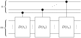
Figure 2: Quantum circuit for a transversal case operator

Proof. We observe that due to binary expansion of the exponent vectors the operation $U^{\oplus}_{T}$ can be implemented as in Figure 2. The statement concerning the number of gates of this factorization follows immediately from the previous lemma.  $\Box$

A familiar example is given by the additive cyclic group ${\mathbb{Z}}/2^{n}{\mathbb{Z}}$. Assume that this group is represented by $D(g)=U^{g}$, where $g\in{\mathbb{Z}}/2^{n}{\mathbb{Z}}$ and $U$ is some unitary matrix satisfying $U^{2^{n}}=\mbox{\bf 1}$. A composition series is given by the subgroups $G_{i}=2^{n-i}{\mathbb{Z}}/2^{n}{\mathbb{Z}}$. A transversal for the group ${\mathbb{Z}}/2^{n}{\mathbb{Z}}$ is, for instance, given by the group elements $t_{i}=2^{n-i}$, that is, $T=(2^{n-1},2^{n-2},\dots,2,1)$. The implementation described in the previous theorem realizes the powers $U^{2^{i}}$. An arbitrary power $U^{g}$ is realized by setting the $n$ control bits according to the binary expansion $g=\sum g_{i}2^{n-i}$, with $g_{i}\in\{0,1\}$.

6 The Design Principle

Suppose that we want to realize a unitary matrix $A\in{\mathcal{U}}(2^{m})$ by a quantum circuit. We assume that some unitary matrices $D(g)\in{\mathcal{U}}(2^{m})$ with efficient quantum circuits are known to us. Familiar examples are discrete Fourier transforms, permutation matrices, and so on. Suppose that some of the matrices $D(g)$ generate a finite dimensional group algebra containing the matrix $A$, then, simply put, a quantum circuit can be found for $A$. The following theorem describes how this can be accomplished. To ease the presentation, we do not state the theorem in its most general form. The more technical generalizations will be discussed in the subsequent sections.

Theorem 5

Let $G$ be a finite group of order $2^{n}$, and denote by $T=(t_{1},\ldots,t_{n})$ a transversal of $G$, that is, each element $g\in G$ can be uniquely represented in the form $g=t_{1}^{a_{1}}\cdot\ldots\cdot t_{n}^{a_{n}}$, where $a_{i}\in\{0,1\}$. Let $D:G\rightarrow{\cal U}(2^{m})$ be a unitary representation of $G$ such that the images $\{D(g):g\in G\}$ form a set of linearly independent unitary operations. Suppose that $A\in{\cal U}(2^{m})$ is a linear combination of the representing matrices $D(g)$,

$$A=\sum_{g\in G}\alpha_{g}D(g),$$

with coefficients $\alpha_{g}\in{\mathbb{C}}$. If $C_{A}={\rm circ}_{G}(\left|\alpha\right>)$ denotes the associated group-circulant, with elements ordered according to the choice of the transversal $T$, then the matrix $A$ is realized by the circuit given in Figure 3.

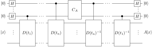
Figure 3: Quantum circuit implementing a linear combination

Proof. Note that by the choice of the transversal $T$ the ordering of the elements of $G$ is fixed. We define $H$ to be the transformation $H:=H_{2}\otimes\ldots\otimes H_{2}\otimes\mbox{\bf 1}_{2^{n}}$, where the first $n$ factors are equal to the Hadamard transform $H_{2}$. The transformation $H$ corresponds to the leftmost and to the rightmost transformation in Figure 3. Furthermore, we define $C_{A}:={\rm circ}(\left|\alpha\right>)\otimes\mbox{\bf 1}_{2^{n}}$ and ${\cal D}:={\rm diag}(D(g_{1}),\ldots,D(g_{2^{n}}))$. Observe that ${\cal D}$, $C_{A}$, and ${\cal D}^{-1}$ are the remaining transformations in Figure 3. The circuits for ${\cal D}$ and ${\cal D}^{-1}$ are shown in factorized form, hereby exploiting the group-structure of the case-operator. We obtain the factorization of ${\cal D}$ as in Figure 2. To verify that the circuit indeed computes $\left|0\right>\left|x\right>\mapsto\left|0\right>A\left|x\right>$, we first consider the matrix identity

$${\cal D}^{-1}\cdot C_{A}\cdot{\cal D}=\left(\begin{array}[]{cccc}\alpha_{g_{1}}\mbox{\bf 1}_{2^{n}}&\alpha_{g_{2}}D(g_{2})&\cdots&\alpha_{g_{2^{n}}}D(g_{2^{n}})\\ \alpha_{g_{2}^{-1}}D(g_{2}^{-1})&\alpha_{g_{1}}\mbox{\bf 1}_{2^{n}}&\cdots&\vdots\\ \vdots&\ddots&\ddots&\vdots\\ \alpha_{g_{2^{n}}^{-1}}D(g_{2^{n}}^{-1})&\cdots&\cdots&\alpha_{g_{1}}\mbox{\bf 1}_{2^{n}}\end{array}\right).$$ (3)

To be more precise, the entry at position $(i,j)$ of this block-structured matrix is equal to $\alpha_{g_{i}^{-1}g_{j}}D(g_{i}^{-1})D(g_{j})=\alpha_{g_{i}^{-1}g_{j}}D(g_{i}^{-1}g_{j})$. This means that each row of blocks of (3) contains the set of matrices $\{\alpha_{g}D(g)\,\colon\,g\in G\}$ in some permuted order. The same holds for the columns of this matrix. Hence we can conclude that the first row of the matrix $H^{-1}{\cal D}^{-1}\cdot C_{A}\cdot{\cal D}$ is given by $\frac{1}{\sqrt{2^{n}}}(\sum_{g}\alpha_{g}D(g),\ldots,\sum_{g}\alpha_{g}D(g))=\frac{1}{\sqrt{2^{n}}}(A,\ldots,A)$. Hence applying $H$ to the columns of this matrix will produce

$$H^{-1}\cdot{\cal D}^{-1}\cdot C_{A}\cdot{\cal D}\cdot H=\left(\begin{array}[]{cc}A&\mbox{\bf 0}\\ \mbox{\bf 0}&U\end{array}\right),$$ (4)

with some unitary matrix $U\in{\cal U}(2^{n+m}{-}2^{m})$ and zero-matrices of the appropriate sizes. Note that the entries in the same rows resp. columns as $A$ must vanish, since $A$ as well as the other operations used in (4) are unitary. $\Box$

Remark. Note that the assumptions in the theorem can be considerably relaxed. The restriction to 2-groups is not necessary. In fact, the implementation of case operators can be extended to arbitrary solvable groups. Moreover, we will show in the next section that the representing matrices $D(g)$ do not need to be linearly independent; one can always find suitable unitary group circulants $C_{A}$. Finally, it is not necessary that the representing matrices form an ordinary representation; the extension to projective representations is discussed in Section 8.

Note that the cost of implementing a circuit for $A$ is determined by the cost of the transversal elements $\kappa(D_{t_{i}})$, $1\leq i\leq n$, and by the cost of the group circulant $\kappa(C_{A})$. If the group $G$ is of small order, say the order is bounded by $c$, then the efficiency of the implementation of a transformation which has been decomposed according to Theorem 5 depends only on the complexity of the transformations $\kappa(D_{t_{i}})$. A family of representations with this property will be studied in Section 10.2.

7 Generalization

The theorem in the previous section assumed that the representing matrices $D(g)$ of the group $G$ are linearly independent. The next theorem shows that one can drop this assumption entirely.

Theorem 6

Let $D\colon G\rightarrow{\mathcal{U}}(2^{n})$ be an ordinary representation of a finite group $G$. If a unitary matrix $A$ can be expressed as a linear combination

$$A=\sum_{g\in G}\alpha_{g}D(g),\qquad\alpha_{g}\in{\mathbb{C}},$$

then the coefficients $\alpha_{g}$ can be chosen such that the associated group circulant is unitary.

Proof. A finite group has a finite number of non-equivalent irreducible representations. Let $D^{(k)}\colon G\rightarrow{\mathcal{U}}(n_{k})$, $k\in I$, be a representative set of the non-equivalent irreducible unitary representations of the finite group $G$.

Let $D_{ij}^{k}\colon G\rightarrow{\mathbb{C}}$ be the complex-valued function on $G$, which is determined by the value of the $(i,j)$-coefficient of the representing matrix $D^{(k)}$. We obtain $\sum_{k\in I}n_{i}^{2}$ functions in this way. It was shown by Schur that these functions are orthogonal,

$$\langle D_{ij}^{k}|D_{i^{\prime}j^{\prime}}^{k^{\prime}}\rangle=0,$$

unless $i=i^{\prime}$, $j=j^{\prime}$, and $k=k^{\prime}$; see [16, Section 2.2].

Denote by

$$J=\{k\in I\colon D^{(k)}\mbox{ is a constituent of the representation }D\}.$$

Let $E$ denote the direct sum of the irreducible representations, which are not contained in $D$, that is,

$$E(g)=\bigoplus_{k\in I-J}D^{(k)}(g).$$

We have

$$A\oplus I=\sum_{g\in G}\alpha_{g}(D(g)\oplus E(g))$$

for some $\alpha_{g}\in{\mathbb{C}}$. Indeed, comparing coefficients yields a system of $|G|$ linear equations. This system of equations can be solved, since the coefficient functions are orthogonal. The circulant corresponding to the coefficients $\alpha_{g}$ is unitary by Theorem 7. Ignoring the representing matrices $E(g)$, we obtain $A$ as a linear combination of the representing matrices $D(g)$, as claimed.  $\Box$

8 Extension to Projective Circulants

We have assumed in Theorem 5 that $A$ is obtained as a linear combination of matrices $D(g)$, which form an ordinary representation of a finite group $G$. It turns out that the quantum circuit used for the implementation of $A$ can also be used, with a minor modification, for projective representations. We recall a few basic facts about projective representations and then give the appropriate generalization of the circulant matrices introduced in Section 4.

Note that projective representations have been used in quantum information theory. They for instance turn out to be the adequate formalism to describe a class of unitary error bases [17].

Let $D\colon G\rightarrow U(n)$ be a projective unitary representation of a finite group $G$ with factor set $\omega$. In other words, $\omega$ is a function from $G\times G$ to the nonzero complex numbers ${\mathbb{C}}^{\times}$ such that

$$D(g)D(h)=\omega(g,h)D(gh)$$ (5)

holds for all $g,h\in G$. The associativity of matrix multiplication implies the relations

$$\omega(x,y)\omega(xy,z)=\omega(x,yz)\omega(y,z)$$ (6)

for all $x,y,z\in G$. This shows that $\omega$ is a $2$-cocycle of the group $G$ with trivial action on ${\mathbb{C}}^{\times}$.

We assume that the neutral element $1$ of the group $G$ is represented by the identity matrix $D(1)=1_{n}$, which implies

$$\omega(g,1)=\omega(1,g)=1\qquad\mbox{for all}\quad g\in G.$$ (7)

The values of the factor system $\omega$ are of modulus 1, since the representation matrices $D(g)$ are unitary. This shows, in particular, the relations

$$\overline{\omega(g,h)}=\omega(g,h)^{-1}\qquad\mbox{for}\quad g,h\in G.$$ (8)

Let $\alpha\in{\mathbb{C}}^{|G|}$ be a vector which is labeled by the elements of $G$. We define a projective group circulant for $(G,\omega)$ with respect to $\alpha$ to be the matrix

$${\rm circ}_{G,\omega}(\alpha)=\left(\,\omega(g^{-1},h)^{-1}\,\alpha_{g^{-1}h}\,\right)_{g,h\in G}.$$

Projective circulants have been introduced by I. Schur [18]. We show that in the analog situation to Theorem 5 the associated projective circulants are unitary.

Theorem 7

Let $D\colon\,G\rightarrow{\cal U}(n)$ be an $n$-dimensional unitary projective representation of a finite group $G$. Suppose that the operators $\{D(g)\colon g\in G\}$ are linearly independent. If a unitary matrix $A\in{\cal U}(n)$ can be expressed as a linear combination

$$A=\sum_{g\in G}\alpha_{g}D(g),\qquad\mbox{with}\quad\alpha_{g}\in{\mathbb{C}},$$

then the projective group circulant ${\rm circ}_{G,\omega}(\alpha)$ of the coefficients $\alpha_{g}$ is unitary.

Proof.  It suffices to show that the rows of the projective group circulant ${\rm circ}_{G,\omega}(\alpha)$ are pairwise orthogonal and of unit length, or more explicitly that

$$\sum_{h\in G}(\omega(g,h)\overline{\omega(k,h)})^{-1}\alpha_{gh}\overline{\alpha_{kh}}=\delta_{g,k}$$ (9)

holds for all $g,k\in G$. We will show that these orthogonality relations can be derived from the matrix identity $AA^{\dagger}D(k)=D(k)$.

Multiplying $A,A^{\dagger}$ and $D(k)$ yields

$$AA^{\dagger}D(k) = \Big{(}\sum_{g\in G}\alpha_{g}D_{g}\Big{)}\Big{(}\sum_{h\in G}\overline{\alpha_{h}}D(h)^{\dagger}\Big{)}D(k)$$

$$= \sum_{g\in G}\sum_{h\in G}\alpha_{g}\overline{\alpha_{h}}D(g)D(h)^{\dagger}D(k).$$

Notice that the multiplication rules (5) imply

$$D(g)D(h)^{\dagger}D(k)=\frac{\omega(g,h^{-1})\omega(gh^{-1},k)}{\omega(h,h^{-1})}D(gh^{-1}k).$$

Therefore, $AA^{\dagger}D(k)=D(k)$ can be expressed as

$$D(k) = \sum_{g\in G}\sum_{h\in G}\alpha_{g}\overline{\alpha_{h}}\frac{\omega(g,h^{-1})\omega(gh^{-1},k)}{\omega(h,h^{-1})}D(gh^{-1}k)$$

$$\stackrel{{\scriptstyle\ell=gh^{-1}}}{{=}} \sum_{\ell\in G}\Big{(}\sum_{h\in G}\alpha_{\ell h}\overline{\alpha_{h}}\frac{\omega(\ell h,h^{-1})\omega(\ell,k)}{\omega(h,h^{-1})}\Big{)}D(\ell k).$$

Setting $x:=\ell$, $y:=h$ and $z:=h^{-1}$ in (6) shows the identity

$$\omega(\ell h,h^{-1})\omega(h,h^{-1})^{-1}=\omega(\ell,h)^{-1},$$

which allows to simplify the previous expression for $D(k)$ to

$$D(k) = \sum_{\ell\in G}\Big{(}\sum_{h\in G}\alpha_{\ell h}\overline{\alpha_{h}}\frac{\omega(\ell,k)}{\omega(\ell,h)}\Big{)}D(\ell k)$$

$$= \sum_{\ell\in G}\Big{(}\sum_{h\in G}\alpha_{\ell kh}\overline{\alpha_{kh}}\frac{\omega(\ell,k)}{\omega(\ell,kh)}\Big{)}D(\ell k).$$

The substitution $g=\ell k$ yields

$$D(k)=\sum_{g\in G}\Big{(}\sum_{h\in G}\alpha_{gh}\overline{\alpha_{kh}}\frac{\omega(gk^{-1},k)}{\omega(gk^{-1},kh)}\Big{)}D(g).$$

Setting $x:=gk^{-1}$, $y:=k$, and $z:=h$ in the cocycle relation (6) shows the identity

$$\frac{\omega(gk^{-1},k)}{\omega(gk^{-1},kh)}=\frac{\omega(k,h)}{\omega(g,h)}.$$

This allows to write $D(k)$ in the form

$$D(k)=\sum_{g\in G}\Big{(}\sum_{h\in G}\frac{\omega(k,h)}{\omega(g,h)}\alpha_{gh}\overline{\alpha_{kh}}\Big{)}D({g})$$

Comparing coefficients on both sides yields

$$\sum_{h\in G}\frac{\omega(k,h)}{\omega(g,h)}\alpha_{gh}\overline{\alpha_{kh}}=\delta_{g,k}\quad\mbox{for all}\quad g,k\in G.$$

Using (8), this shows that the orthogonality relations (9) hold. Thus, the projective group circulant ${\rm circ}_{G,\omega}(\alpha)$ is indeed unitary, as claimed.  $\Box$

We remark that a theorem analogous to Theorem 5 holds in the situation where $D$ is a projective representation of a finite group $G$. In this case the matrices $D_{t_{i}}$ have to be replaced by a suitably rescaled transversal and the circulant matrix $C_{A}$ has to be replaced by the corresponding projective circulant. Theorem 7 guarantees that the latter matrix is unitary.

Using projective representations a greater flexibility can be achieved. In Section 10.3 we give an example for a projective representation of the group ${\mathbb{Z}}_{2}\times{\mathbb{Z}}_{2}$ which is given by the Pauli matrices.

9 Relation to Kitaev’s algorithm

Kitaev presented in [19] and [20] a quantum circuit that allows to estimate an eigenvalue of a unitary matrix provided that the corresponding eigenstate is given; see also [21] and [22] for further descriptions of this scenario. The phase estimation provides a unified framework for Shor’s algorithm [3] and the algorithms for abelian stabilizers [19, 23]. In the following we give a brief account of this method. Starting from a unitary transformation $U$ on $n$ qubits and an eigenvector $\left|\psi_{\lambda}\right>$, we want to generate an estimate of $\lambda$. The precision of this approximation is controlled by the number $k$ of digits we want to compute in the binary expansion $\lambda=0.\,b_{1}\,b_{2}\,b_{3}\,\ldots$ of $\lambda$, i. e., $b_{i}\in{\mathbb{F}}_{2}$.

If we assume that, in addition to $U$ and $\left|\psi_{\lambda}\right>$, we are given efficient quantum circuits implementing $\Lambda_{1}(U^{2^{j}})$ for $j=0,\ldots,k-1$, then it is possible to accomplish the task of approximating $\lambda$ by means of an efficient quantum circuit. This circuit, which is given in Figure 4, consists of three parts.

Reading from left to right, we have a quantum circuit acting on two registers: the first holds the eigenstate $\left|\psi_{\lambda}\right>$ and the second, which ultimately will contain the approximation $|\tilde{\lambda}\rangle$, is initialized with the $\left|0\right>$ state. In a first step an equal-weighted superposition of all binary strings on the second register is generated by application of a Hadamard transform to each wire. Then the transformation $U^{\oplus}:=\left|i\right>\left|x\right>\mapsto\left|i\right>U^{i}\left|x\right>$ is performed for $i=0,\ldots,2^{k}-1$. Note that if $U$ has finite order $2^{k}$, then $U^{\oplus}$ is a case-operator (in the sense of Section 5) for the cyclic group $Z_{2^{k}}$. In a third step an inverse Fourier transform $F_{2^{k}}^{-1}$ is computed giving the best $k$-bit approximation of $\lambda$ which is stored in the second register [21].

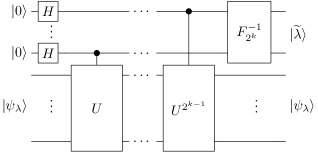
Figure 4: Quantum circuit for eigenvalue estimation

The connection between the algorithm for phase estimation and the circuit given in Figure 3 is established as follows. For the special case of $G={\mathbb{Z}}/{2^{k}}{\mathbb{Z}}$ generated by a unitary transformation $U\in{\cal U}(2^{n})$ of order $2^{k}$ we first apply the circuit given in Figure 4 to each element of a basis $\{\left|\psi_{i}\right>:i=1,\ldots,2^{k}\}$ of eigenvectors of $U$ in order to obtain the (exact) eigenvalues $\lambda_{i}$ in the second register. Note that there are at most $2^{k}$ different eigenvalues of $U$. We then perform the scalar multiplication $\lambda_{i}\mapsto\alpha_{i}\lambda_{i}$ for certain $\alpha_{i}\in{\cal U}(1)$ and all $i=1,\ldots,2^{k}$. Finally we run the circuit given in Figure 4 backwards and observe that

$$F_{2^{k}}^{-1}\cdot{\rm diag}(\alpha_{1},\ldots,\alpha_{2^{k}})\cdot F_{2^{k}}={\rm circ}_{{\mathbb{Z}}/{2^{k}}{\mathbb{Z}}}(\beta_{1},\ldots,\beta_{2^{k}}),$$

where the vector $\left|\beta\right>=(\beta_{1},\ldots,\beta_{2^{k}})\in{\mathbb{C}}^{2^{k}}$ is given by $\left|\beta\right>=F_{2^{k}}\left|\alpha\right>$. Here $F_{N}=[e^{2\pi ikl/N}]_{k,l=0,\ldots,N-1}$ denotes the (unnormalized) discrete Fourier transform.

Note, that the method presented in Section 6 is more general than this twofold application of the circuit for eigenvalue estimation as it allows to work with representations of arbitrary finite groups.

10 Examples

The decomposition method introduced in the previous sections is demonstrated by means of the Hartley transforms which have been introduced in Section 3 and fractional Fourier transforms (cf. [24, 25]) which are a class of unitary transformations used in classical signal processing. Using the method of linear combinations of unitary operations we show how to compute them efficiently on a quantum computer. Finally, we show that the quantum circuit for teleportation of a qubit can be interpreted with the help of this method.

10.1 Hartley Transforms Revisited

The efficient quantum circuit shown in Figure 1 of Section 3 can be recast in terms of Theorem 5. First recall that the identity

$$A_{N}=\alpha\;F_{N}+\beta\;F_{N}^{3}$$

with $\alpha:=\left(\frac{1-i}{2}\right)$ and $\beta:=\left(\frac{1+i}{2}\right)$ shows that the Hartley transform $A_{N}$ is a linear combination of the powers $\mbox{\bf 1}_{N},F_{N},F_{N}^{2},F_{N}^{3}$ of the discrete Fourier transform $F_{N}$. We can simplify this to obtain $A_{N}=F_{N}\tilde{A}_{N}$, where $\tilde{A}_{N}$ is defined as $\tilde{A}_{N}:=\alpha\mbox{\bf 1}_{N}+\beta F_{N}^{2}$. Since $F_{N}^{2}$ is an involution, we can apply apply Theorem 5 in the special situation where $|G|=2$. Hence the circulant $C_{\tilde{A}_{N}}$ is in this case the ${\mathbb{Z}}/2{\mathbb{Z}}$ circulant matrix

$$R:=\frac{1}{2}\left(\begin{array}[]{rr}1-i&1+i\\ 1+i&1-i\end{array}\right).$$

Since for $N\geq 5$ the matrices $\mbox{\bf 1}_{N},F_{N},F_{N}^{2},F_{N}^{3}$ are linearly independent, we can use Theorem 5 to conclude that $R$ has to be unitary. Hence we can implement $\tilde{A}_{N}$ using one auxiliary qubit with a quantum circuit as in Figure 3. Combining the circuits for $F_{N}$ and for $\tilde{A}_{N}$ we finally obtain the factorization of $A_{N}$ shown in Figure 1 of Section 3.

10.2 Fractional Fourier Transforms

A matrix $A$ having the property $A^{\alpha}=B$ with $\alpha\in{\mathbb{R}}$ is called an $\alpha$-th root of $B$ (where in general this root is not uniquely determined). In case of the discrete Fourier transform $F_{N}$ we can use the property that $F_{N}^{4}=\mbox{\bf 1}_{N}$ to define an $\alpha$-th root of $F_{N}$ via

$$F_{N,\alpha}:=a_{0}(\alpha)\cdot\mbox{\bf 1}_{N}+\ldots+a_{3}(\alpha)\cdot F_{N}^{3},$$ (10)

where the coefficients $a_{i}(\alpha)$ for $i=0,\ldots,3$ are defined by

$$\begin{array}[]{l@{,\;\;}l}a_{0}(\alpha):=\frac{1}{2}(\phantom{{-}}1{+}e^{i\alpha})\cos{\alpha}&a_{1}(\alpha):=\frac{1}{2}(\phantom{{-}}1{-}ie^{i\alpha})\sin{\alpha},\\ a_{2}(\alpha):=\frac{1}{2}({-}1{+}e^{i\alpha})\cos{\alpha}&a_{3}(\alpha):=\frac{1}{2}({-}1{-}ie^{i\alpha})\sin{\alpha}.\\ \end{array}$$

Note that like in the previous example of the discrete Hartley transforms in Section 10.1, we have used the property that $F_{N}$ generates a finite group of order four to obtain the linear combination shown in eq. (10).

It was shown in [24] that the one-parameter family $\{F_{N,\alpha}\;|\;\alpha\in{\mathbb{R}}\}\subset{{\mathbb{C}}}^{N\times N}$ has the following properties:

• $F_{N,\alpha}$ is a unitary matrix for $\alpha\in{\mathbb{R}}$.

• $F_{N,0}=\mbox{\bf 1}_{N}$ and $F_{N,\pi/2}=F_{N}$.

• $(F_{N,\alpha})^{1/\alpha}=F_{N}$ for $\alpha\in{\mathbb{R}}$.

• $F_{N,\alpha}\cdot F_{N,\beta}=F_{N,{\alpha+\beta}}$, for $\alpha,\beta\in R$.

Using Theorem 3 we immediately obtain that $F_{2^{n},{\alpha}}$ can be computed in $O(n^{2})$ elementary quantum operations for all $\alpha\in{\mathbb{R}}$, since the complexity of the discrete Fourier transform $F_{2^{n}}$ of length $2^{n}$ is $O(n^{2})$ (cf. [26, 3]) and the circulant matrix appearing in this case is $C_{\alpha}:={\rm circ}(a_{0}(\alpha),\ldots,a_{3}(\alpha))$ which can be implemented in $O(1)$. More precisely we have

$$C_{\alpha}={\rm circ}(\left|\alpha\right>)=F_{4}^{-1}\cdot{\rm diag}(1,e^{-i\alpha},e^{2i\alpha},e^{-i\alpha})\cdot F_{4}.$$

Using the results of [4] we can reduce the computational complexity of $F_{2^{n}}$ to $O(n(\log n)^{2}\log\log n)$ if we have no restrictions on the number of ancilla qubits.

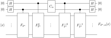
Figure 5: Quantum circuit realizing a fractional quantum Fourier transform

Hence, we obtain the following theorem which summarizes the complexity of computing a fraction Fourier transform.

Theorem 8

Let $\alpha\in{\mathbb{R}}$ and $F_{2^{n},\alpha}$ be the fractional Fourier transform of length $2^{n}$ and parameter $\alpha$. Then $\kappa_{\rm anc}(F_{2^{n},\alpha})=O(n(\log n)^{2}\log\log n)$.

10.3 Teleportation Revisited

In this section, we show how the well-known quantum circuit for teleportation of an unknown quantum state (cf. [27, 28]) can be interpreted with the help of our method. The essential feature of the circuit in Figure 3 is that a measurement on the upper quantum bits can be carried out immediately after the transformation $C_{A}$ has been performed. This has the advantage that the transformations $D(t_{n})^{-1}$ etc. can be classically conditioned. This explains the classical communication part of the teleportation circuit. To obtain the EPR states and the Bell measurement we use some easy reformulations of the transformations exploiting the nature of the projective circulant in case of $2\times 2$ matrices.

Suppose that Alice wants to teleport a quantum state $\left|\psi\right>=\alpha\left|0\right>+\beta\left|1\right>$ of a qubit in her possession to a qubit in Bob’s possession at a remote destination. If the destination qubit is in the state $\left|0\right>$, then, conceptually, the task is to apply a unitary operation $U$ such that $U\left|0\right>=\left|\psi\right>$. Specifically, the matrix $U$ can be chosen to be of the form

$$U=\left(\begin{array}[]{rr}\alpha&\overline{\beta}\\ \beta&-\overline{\alpha}\end{array}\right),\quad\text{where}\;|\alpha|^{2}+|\beta|^{2}=1.$$

Clearly, it would not be feasible for Alice to communicate the specification of $U$ to Bob by classical communication. Therefore, she has to proceed in a different way.

Recall that the matrices

$$\mbox{\bf 1}_{2}=\left(\begin{array}[]{cc}1&0\\ 0&1\end{array}\right),\;\sigma_{x}=\left(\begin{array}[]{cc}0&1\\ 1&0\end{array}\right),\;\sigma_{z}=\left(\begin{array}[]{rr}1&0\\ 0&-1\end{array}\right),\;\sigma_{x}\sigma_{z}=\left(\begin{array}[]{ll}0&-1\\ 1&\phantom{-}0\end{array}\right).$$

form a basis ${\cal B}=\{\mbox{\bf 1}_{2},\sigma_{x},\sigma_{z},\sigma_{x}\sigma_{z}\}$ of the vector space of complex $2\times 2$ matrices. Thus, the matrix $U$ can be written as a linear combination $U=\sum_{B\in{\cal B}}c_{B}B$. Note that the Pauli basis ${\cal B}$ is an orthonormal basis of ${\mathbb{C}}^{2\times 2}$ with respect to the inner product $\langle B|A\rangle=\frac{1}{2}\mbox{tr}(B^{\dagger}A)$. As a result, the coefficient $c_{B}$ corresponding to $B\in{\cal B}$ can be easily computed by $c_{B}=\frac{1}{2}{\rm tr}(B^{\dagger}U)$. Consequently, we obtain

$$U=\left(\frac{\alpha-\overline{\alpha}}{2}\right)\mbox{\bf 1}_{2}+\left(\frac{\beta+\overline{\beta}}{2}\right)\sigma_{x}+\left(\frac{\alpha+\overline{\alpha}}{2}\right)\sigma_{z}+\left(\frac{\beta-\overline{\beta}}{2}\right)\sigma_{x}\sigma_{z}.$$ (11)

The Pauli matrices define a projective representation of the abelian group ${\mathbb{Z}}/2{\mathbb{Z}}\times{\mathbb{Z}}/2{\mathbb{Z}}$ (see, e. g., [17]). Applying the method described in Section 8, the decomposition (11) gives rise to the projective circulant matrix $C_{U}$ defined as follows:

$$C_{U}=\frac{1}{2}\left(\begin{array}[]{rrrr}\alpha-\overline{\alpha}&\beta+\overline{\beta}&\alpha+\overline{\alpha}&\beta-\overline{\beta}\\[2.15277pt] \beta+\overline{\beta}&\alpha-\overline{\alpha}&\beta-\overline{\beta}&\alpha+\overline{\alpha}\\[2.15277pt] \alpha+\overline{\alpha}&-(\beta-\overline{\beta})&\alpha-\overline{\alpha}&-(\beta+\overline{\beta})\\[2.15277pt] \beta-\overline{\beta}&-(\alpha+\overline{\alpha})&\beta+\overline{\beta}&-(\alpha-\overline{\alpha})\end{array}\right).$$

We can express $C_{U}$ by a sequence of Hadamard gates, controlled-not gates, and the single-qubit gate $U$. Indeed, a straightforward calculation shows that

$$(H\otimes\mbox{\bf 1}_{2})\,C_{U}\,(H\otimes\mbox{\bf 1}_{2})=\left(\begin{array}[]{rrrr}\alpha&0&0&\overline{\beta}\\[2.15277pt] \beta&0&0&-\overline{\alpha}\\[2.15277pt] 0&\beta&-\overline{\alpha}&0\\[2.15277pt] 0&\alpha&\overline{\beta}&0\end{array}\right)=:\widetilde{C_{U}}.$$

Applying suitable permutations from the left and the right to the matrix $\widetilde{C_{U}}$ we finally obtain the expression

$${\rm CNOT}^{(1,2)}\,{\rm CNOT}^{(2,1)}\,\widetilde{C_{U}}\,{\rm CNOT}^{(2,1)}=U\otimes\mbox{\bf 1}_{2}.$$ (12)

Overall we obtain that $C_{U}$ is given by the circuit shown in Figure 6.

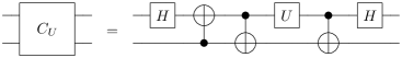
Figure 6: Realisation of the projective circulant $C_{U}$ in terms of the operations $U$, controlled-not gates, and the Hadamard transform $H$.

We now turn to the circuit implementing the transformation $U$ using the linear combination (11). In the following we will modify the generic circuit step by step using elementary identities of quantum gates. We start with the identity

which is obtained directly from the method of Sections 6 and 8. The matrix $U$ is given by a linear combination of Pauli matrices in eq. (11). This limear combination determines $C_{U}$. We rewrite $C_{U}$ as a product of CNOT gates and local unitary transformations using eq. (12). We obtain the circuit

where we also turned the first controlled-$\sigma_{z}$ gate upside down. Now we can use the basic fact that $H\sigma_{z}H=\sigma_{x}$ to rewrite the controlled-$\sigma_{z}$ framed by the two Hadamard gates on the top wire in the following way:

We can simplify the sequence of the first five gates of the last circuit. Indeed, since we start from the state $\left|0\right>\left|0\right>\left|0\right>$, the state resulting from applying the first five gates is $\left|0\right>(\left|00\right>+\left|11\right>)$. This state can be obtained by applying the first two of these five gates alone. This simplification yields the following circuit

which decomposes into three stages: (i) EPR pair and state preparation in which, starting from the ground state $\left|0\right>\left|0\right>\left|0\right>$, two of the bits are turned into an EPR state while the third qubit holds the unknown state $\left|\psi\right>$, (ii) Bell measurement of the two most significant qubits, and (iii) a reconstruction operation which is a conditional transformation on qubit one depending on the outcome of the measurement of qubits two and three.

Hence, this circuit equals the teleportation circuit for an unknown quantum state $\left|\psi\right>=U\left|0\right>$, see for instance [28, Section 1.3.7] or [27]. In summary, we have seen that it is possible to derive a transformation of a quantum circuit corresponding to linear combination of the transformation $U$ as a sum of Pauli matrices into the teleportation circuit.

11 Conclusions

The factorization of a unitary matrix in terms of elementary quantum gates amounts to solve a word problem in a unitary group. This problem is quite difficult, in particular since only words of small length, which correspond to efficient algorithms, are of practical interest. Few methods are known to date for the design of quantum circuits. Several ad-hoc methods for quantum circuit design have been proposed, mostly heuristic search techniques based on genetic algorithms, simulated annealing or the like. Such methods are confined to fairly small circuit sizes, and the solutions produced by such heuristics are typically difficult to interpret.

The method presented in this paper follows a completely different approach. We assume that we have a set of efficient quantum circuits available. Our philosophy is to reuse and combine these circuits to build a new quantum circuit. We have developed a sound mathematical theory, which allows to solve such problems under certain well-defined conditions. Following this approach, we have demonstrated that the discrete Hartley transforms and fractional Fourier transforms have extremely efficient realizations on a quantum computer.

It should be stressed that the method is by no means exhausted by these examples. From a practical point of view, it would be interesting to build a database of moderately sized matrix groups which have efficient quantum circuits. This database could in turn be searched for a given transformation by means of linear algebra. It is an appealing possibility to automatically derive quantum circuit implementations in this fashion.

Acknowledgements

The research of A.K. has been partly supported by NSF grant EIA 0218582, and by a Texas A&M TITF grant. Part of this work has been done while M.R. was at the Institute for Algorithms and Cognitive Systems, University of Karlsruhe, Karlsruhe, Germany, and during a visit to the Mathematical Sciences Research Institute, Berkeley, USA. He wishes to thank both institutions for their hospitality. His research has been supported by the European Community under contract IST-1999-10596 (Q-ACTA), CSE, and MITACS.

References

References

- [1] A. Barenco, C. H. Bennett, R. Cleve, D. P. DiVincenzo, N. Margolus, P. Shor, T. Sleator, J. A. Smolin, and H. Weinfurter. Elementary gates for quantum computation. Physical Review A, 52(5):3457–3467, November 1995.
- [2] G. Alber, Th. Beth, M. Horodecki, P. Horodecki, R. Horodecki, M. Rötteler, H. Weinfurter, R. Werner, and A. Zeilinger. Quantum Information: An Introduction to Basic Theoretical Concepts and Experiments, volume 173 of Springer Texts in Modern Physics. Springer, 2001.
- [3] P. W. Shor. Algorithms for quantum computation: discrete logarithm and factoring. In Proc. FOCS 94, pages 124–134. IEEE Computer Society Press, 1994.
- [4] R. Cleve and J. Watrous. Fast parallel circuits for the quantum Fourier transform. Technical report, LANL preprint quant-ph/0006004, 2000.
- [5] M. Ettinger. Quantum time-frequency transforms. LANL preprint quant–ph/0005134, 2000.
- [6] P. Høyer. Efficient quantum transforms. LANL preprint quant–ph/9702028, February 1997.
- [7] A. Klappenecker. Wavelets and wavelet packets on quantum computers. In M.A. Unser, A. Aldroubi, and A.F. Laine, editors, Wavelet Applications in Signal and Image Processing VII, pages 703–713. SPIE, 1999.
- [8] A. Klappenecker and M. Rötteler. Discrete cosine transforms on quantum computers. In Proc. IEEE R8-EURASIP Symposium on Image and Signal Processing and Analysis (ISPA01), Pula, Croatia, 2001.
- [9] M. Püschel, M. Rötteler, and Th. Beth. Fast quantum Fourier transforms for a class of non-abelian groups. In Proceedings Applied Algebra, Algebraic Algorithms and Error-Correcting Codes (AAECC-13), volume 1719 of Lecture Notes in Computer Science, pages 148–159. Springer, 1999.
- [10] Th. Beth. Generating fast Hartley transforms - another application of the algebraic discrete Fourier transform. In Proc. URSI-ISSSE ’89, pages 688–692, 1989.
- [11] Bracewell. The Hartley Transform. Cambridge Univ. Press, 1979.
- [12] M. Clausen and U. Baum. Fast Fourier Transforms. BI-Verlag, 1993.
- [13] P. Davis. Circulant matrices. Wiley-Interscience New York, 1979.
- [14] B. Huppert. Endliche Gruppen I. Grundlehren der mathematischen Wissenschaften. Springer-Verlag, Berlin, 1979.
- [15] D. DiVincenzo. Quantum gates and circuits. Proc. R. Soc. London A, 454(1969):261–276, 1998.
- [16] J.P. Serre. Linear Representations of Finite Groups, volume 42 of GTM. Springer-Verlag, Berlin, 1996. (5th corr. printing).
- [17] A. Klappenecker and M. Rötteler. Beyond Stabilizer Codes I: Nice Error Bases. IEEE Transactions on Information Theory, 48(8):2392–2395, 2002.
- [18] I. Schur. Beiträge zur Theorie der Gruppen linearer homogener Substitutionen. Trans. Amer. Math. Soc., 10:159–175, 1909.
- [19] A. Yu. Kitaev. Quantum measurements and the abelian stabilizer problem. LANL preprint quant–ph/9511026, November 1995.
- [20] A. Yu. Kitaev. Quantum computations: algorithms and error correction. Russian Math. Surveys, 52(6):1191–1249, 1997.
- [21] Cleve, R. and Ekert, A. and Macchiavllo, C. and Mosca, M. Quantum algorithms revisited. Proceedings of the Royal Society of London (Series A), 454(1969):339–354, 1998.
- [22] R. Jozsa. Quantum algorithms and the Fourier transform. Proc. R. Soc. Lond. A, 454:323–337, 1998.
- [23] D. Grigoriev. Testing shift-equivalence of polynomials using quantum machines. In Proc. International Symposium on Symbolic and Algebraic Computation (ISSAC), pages 49–54. ACM Press, 1996.
- [24] S. Balasubramaiam and J. McClellan. The discrete rotational Fourier transform. IEEE Transactions on Signal Processing, 44(4):994–998, 1996.
- [25] C. Candan, M. Kutay, and H. Ozaktas. The discrete fractional Fourier transform. IEEE Transactions on Signal Processing, 48(5):1329–1337, 2000.
- [26] D. Coppersmith. An approximate Fourier transform useful for quantum factoring. Technical Report RC 19642, IBM Research Division, 1994. see also LANL preprint quant-ph/0201067.
- [27] G. Brassard, S. Braunstein, and R. Cleve. Teleportation as a quantum computation. Physica D, 120(1–2):43–47, 1998.
- [28] M. Nielsen and I. Chuang. Quantum Computation and Quantum Information. Cambridge University Press, 2000.