Unusual quantum states: nonlocality, entropy, Maxwell’s daemon, and fractals

Abstract

energy conservation; nonlocality; quantum measurement; Bell inequality; fractals; von Neumann entropy; Maxwell’s daemon This paper analyses the mathematical properties of some unusual quantum states that are constructed by inserting an impenetrable barrier into a chamber confining a single particle. If the barrier is inserted at a fixed node of the wave function, then the energy of the system is conserved. After barrier insertion, a measurement is made on one side of the chamber to determine if the particle is physically present. The measurement causes the wave function to collapse, and the energy that was contained in the subchamber in which the particle is now absent transfers instantaneously to the other subchamber in which the particle now exists. This thought experiment constitutes an elementary example of an EPR experiment based on energy conservation rather than momentum or angular momentum conservation. A more interesting situation arises when one inserts the barrier at a point that is not a fixed node of the wave function because this process changes the energy of the system; the faster the barrier is inserted, the greater the change in the energy. At the point of a sudden insertion the energy density becomes infinite; this energy instantly propagates across the subchamber and causes the wave function to become fractal. If an energy measurement is carried out on such a fractal wave function, the resulting mixed state has finite nonzero entropy. Fractal mixed states having unbounded entropy are also constructed and their properties are discussed. For an adiabatic insertion of the barrier, Landauer’s principle is shown to be insufficient to resolve the apparent violation of the second law of thermodynamics that arises when a Maxwell daemon is present. This problem is resolved by calculating the energy required to insert the barrier.

1 Introduction

The Hamiltonian describing a particle of mass $m$ trapped in a one-dimensional infinite square well of width $L$ is

$$H=-\frac{\hbar^{2}}{2m}\frac{\rd^{2}}{\rd x^{2}}$$ (1)

with the boundary conditions that the wave function $\psi(x)$ vanish at $x=0$ and $x=L$. The stationary states and the corresponding energy eigenvalues are

$$\phi_{n}(x)=\sqrt{\frac{2}{L}}\sin\left(\frac{n\pi x}{L}\right)\quad{\rm and}\quad E_{n}=\frac{\pi^{2}\hbar^{2}n^{2}}{2mL^{2}}.$$ (2)

The main purpose of this paper is to investigate the effect of inserting an impenetrable barrier at a point $x_{0}=L-\delta$ inside the potential well. A related investigation for $x_{0}=L/2$ using high-temperature quantum states was done by Zurek (1986) in his study of Maxwell’s daemon. Our objective here is to provide a thorough analysis of the effects of barrier insertion for arbitrary $x_{0}$. Inserting an impenetrable barrier divides the chamber into two noninteracting subchambers. If there is a particle in the original undivided chamber, then after inserting the barrier, this particle can only be present in a classical sense in one of the two subchambers. Quantum mechanically, after the barrier is inserted, the wave function of the particle remains nonzero in both subchambers. We thus consider what happens if we perform a measurement that determines the presence or absence of the particle in a given subchamber. Such a measurement requires a probe, which we treat classically.

The probe: As a simple classical probe we use movable walls at the ends of each of the subchambers (these walls are treated as classical objects). A quantum particle in a subchamber exerts a force on the walls of the chamber (Bender et al. 2002). By pushing on a wall we either detect a force or not and thus we measure the presence or the absence of the particle.

For a given initial state $\psi(x,0)$ of the system, there are two possibilities for the insertion point $x_{0}$ of the barrier; namely, the fixed nodes of the wave function and all other locations. By a fixed node we mean a point $x_{0}$ for which the time-dependent wave function satisfies $\psi(x_{0},t)=0$ for all $t\geq 0$.

Case 1: Inserting an impenetrable barrier at a fixed node. Because the wave function vanishes at the insertion point, the system cannot detect and therefore does not resist the insertion of a barrier. Thus, inserting a barrier does not change the energy of the system. After the insertion, the initial energy is distributed between the two subchambers, one to the left and the other to the right of the barrier. We remark that the wave function cannot collapse to zero in either of the subchambers during the barrier insertion because, if it did, the entropy of the system would be reduced without doing any work.

Case 2: Inserting an impenetrable barrier at a point that is not a fixed node. In this case inserting a barrier changes the energy by an amount that depends on the rate at which the barrier is inserted. The time evolution of the system after the insertion of the barrier depends on how rapidly the barrier is inserted.

In §2 and 3 we examine Case 1 and study the effect of a measurement that determines which side of the inserted barrier the particle is present. Based on the conventional collapse hypothesis of quantum mechanics, we argue that the energy in the subchamber where the particle is found to be absent transfers instantaneously to the other subchamber even if the two subchambers are first separated adiabatically by a great distance. This phenomenon of energy transfer is analogous to the instantaneous transfer of angular momentum in an EPR experiment.

When the barrier is not inserted at a fixed node (Case 2), the analysis becomes more elaborate. We consider in §4 what happens when the insertion is carried out instantaneously. After the insertion it is natural to expand the initial wave function $\psi(x,0)$ in the regions $[0,L-\delta)$ and $(L-\delta,L]$ separately as Fourier series. The orthonormal basis elements in each of the two regions are eigenstates of the Hamiltonians for each of the subchambers. It is shown that a naive calculation of the energy in terms of the expansion coefficients of the wave function gives a divergent expression. This happens because while the series expansion of the initial wave function is convergent, it is not uniformly convergent and thus the series exhibits the Gibbs phenomenon.

Calculating the expectation value of the Hamiltonian requires that the series representing the wave function be twice differentiated. However, one cannot differentiate a nonuniformly convergent Fourier series term by term. By introducing a simple renormalisation scheme we overcome the nonuniform convergence and obtain a finite answer for the expectation value of the Hamiltonian on each side of the barrier. When the resulting expectation values are added, we find that this agrees with the initial energy of the system. However, this calculation still does not determine the total energy because the result does not include the energy density at the insertion point $x_{0}$. At $x_{0}$ the wave function is discontinuous, and consequently the energy density at $x_{0}$ is infinite at the time $t=0^{+}$ immediately after the barrier is inserted. Evidently, it requires an infinite amount of work to insert an impenetrable barrier at a point where there is no fixed node. The effect of a measurement to determine which subchamber contains the particle after a rapid insertion of the barrier is considered in §5.

When an initial state created by the instantaneous insertion of a barrier evolves in time, the discontinuity at $x_{0}$ instantly disappears, and the wave function becomes continuous and square-integrable. However, an infinite amount of energy is stored inside the well and, as a result, the wave function becomes fractal. Thus, the wave function, expressed as a linear combination of the energy eigenstates, no longer belongs to the domain of the Hamiltonian although it remains in the domain of the unitary time evolution operator. In §6 we show that the quantum states encountered here resemble the fractal wave functions introduced by Berry (1996).

In §7 we consider an adiabatic insertion of the barrier. A slow insertion requires only a finite amount of energy, and in the adiabatic limit this energy can be calculated explicitly. In §8 we contrast our results on adiabatic insertion with the work of Zurek (1986) on Maxwell’s daemon. We show that the argument of Zurek about memory erasure of the daemon to support the second law of thermodynamics is insufficient when the barrier is not inserted at the centre of the well.

If we measure the energy of the particle described by a fractal wave function created by an instantaneous insertion of the barrier, the resulting mixed state has finite nonzero von Neumann entropy. We extend this analysis in §9 by constructing a new class of fractal wave functions for which the density matrix of the state has unbounded entropy. Such a state might be obtained by an instantaneous compression, as opposed to an instantaneous division, of the chamber.

In gravitational physics the black-hole surface area provides a bound on entropy. Thus, the existence of a quantum state having unbounded von Neumann entropy in a finite-size quantum well seems to imply that nonrelativistic quantum mechanics can violate the entropy bound of gravitational physics (which in itself would not be surprising). However, the infinite-entropy quantum state introduced in §9 also possesses infinite energy. More generally, we argue in §10 that for a broad class of potentials, any quantum state having infinite entropy must also have infinite energy and/or infinite characteristic size. In §11 we discuss the consequences of separating the two subchambers that are formed after a barrier is inserted. We conclude in §12 with some open issues.

2 Barrier insertion at a fixed node

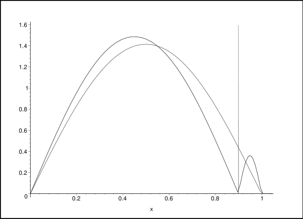
In this section we determine the effect of inserting an impenetrable barrier at a fixed node of the initial wave function. Any of the energy eigenstates other than the ground state has fixed nodes. Furthermore, a superposition of energy eigenstates can also have fixed nodes. As an example, let us choose the initial state

$$\psi(x,0)=\mbox{$\textstyle\frac{1}{\sqrt{2}}$}[\phi_{3}(x)+\phi_{6}(x)].$$ (3)

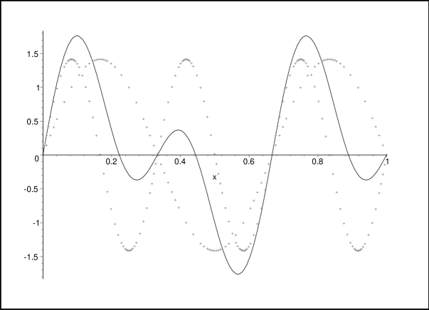
Using (2) we see that the initial energy of the system described by (3) is $\frac{45}{2}(\pi^{2}\hbar^{2}/2mL^{2})$. As shown in Fig. 1, this initial state has nodes at $x/L=0,\frac{2}{9}$, $\frac{1}{3}$, $\frac{4}{9}$, $\frac{2}{3}$, $\frac{8}{9}$, $1$. However, the nodes at $\frac{2}{9}$, $\frac{4}{9}$, $\frac{8}{9}$ are not fixed because the value of the time-dependent wave function $\psi(x,t)$ does not remain zero at these points.

Let us insert an impenetrable barrier at one of the fixed nodes, say $x_{0}=\frac{2}{3}L$, at time $t=0$. The value of $L$ is irrelevant to the discussion here, so we set $L=1$ in this section. Because the inserted barrier is impenetrable, the two subregions can be treated separately. In fact, these two regions can even be moved apart without affecting the states if the separation is done adiabatically. Nevertheless, the state of the system as a whole is described by a single entangled wave function.

The Hamiltonian describing each subregion is the same as that in (1) with the new boundary conditions being that the wave functions must vanish at $x=0$ and at $x=2/3$ in the first subregion and at $x=2/3$ and at $x=1$ in the second subregion. The eigenstates

$$\chi_{n}(x)=\sqrt{3}\sin\left(\mbox{$\textstyle\frac{3}{2}$}\pi nx\right)\quad{\rm and}\quad\eta_{n}(x)=\sqrt{6}\sin\left[3\pi n(x-\mbox{$\textstyle\frac{2}{3}$})\right]$$ (4)

of the Hamiltonians in these two regions constitute orthonormal sets of basis elements in each of the regions $[0,\frac{2}{3}]$ and $[\frac{2}{3},1]$. Therefore, the initial state is

$$\psi(x,0)=\left\{\begin{array}[]{ll}\mbox{$\textstyle\frac{1}{\sqrt{3}}$}\left[\chi_{2}(x)+\chi_{4}(x)\right]&(0\leq x\leq\frac{2}{3}),\\ \mbox{$\textstyle\frac{1}{\sqrt{6}}$}\left[\eta_{1}(x)+\eta_{2}(x)\right]&(\frac{2}{3}\leq x\leq 1).\end{array}\right.$$ (7)

Note that the wave function is not normalised in either region.

Figure 1: The plot of the initial wave function in (3), $\psi(x,0)=\frac{1}{\sqrt{2}}[\phi_{3}(x)+\phi_{6}(x)]$, for $L=1$. The dotted lines represent the two eigenstates $\phi_{3}(x)$ and $\phi_{6}(x)$. The nodes that are common to both eigenstates are the fixed nodes of $\psi(x,t)$. The other nodes of $\psi(x,0)$ are unstable in the sense that $\psi(x,t)$ does not continue to vanish at these points.

Let us calculate the expectation value of the Hamiltonian. The energy eigenvalues in each region are $E_{n}^{\chi}=\frac{9}{4}n^{2}(\pi^{2}\hbar^{2}/2m)$ and $E_{n}^{\eta}=9n^{2}(\pi^{2}\hbar^{2}/2m)$, respectively. Using the basis decomposition (7) the energy expectation values for each side of the barrier are $E_{\chi}=\frac{45}{3}(\pi^{2}\hbar^{2}/2m)$ and $E_{\eta}=\frac{45}{6}(\pi^{2}\hbar^{2}/2m)$. Thus, $E_{\chi}+E_{\eta}=\frac{45}{2}(\pi^{2}\hbar^{2}/2m)$, which is just the initial energy of the system. Because the energy expectation is a constant under unitary time evolution the expectation value obtained from the time-dependent wave function $\psi(x,t)$ gives the identical result. Analogous results hold for all other initial pure states, and we conclude that inserting an impenetrable barrier at a fixed node requires no energy.

3 Wave-function collapse and nonlocal energy transfer

What happens if we observe whether the particle is present in one of the two subregions, say $[\frac{2}{3},1]$ after we have inserted an impenetrable barrier? As discussed in §1, the thought experiment that we have in mind consists of detecting whether there is a force on the wall of the subchamber. If the particle is trapped in the range $[\frac{2}{3},1]$, then we can detect the force that the particle exerts on the wall of the subchamber.

Our concern here is how such a measurement affects the energy of the system. We have established in the previous section that prior to the measurement the energy is distributed among the two separate subregions, even though there is only one particle. Let us suppose that the measurement confirms the absence of the particle in the range $[\frac{2}{3},1]$. Such an outcome occurs with probability $\frac{1}{3}$. After this measurement we can infer that the value of $E_{\eta}$ is now zero. This appears to be paradoxical unless we can explain where the energy has gone.

How does this measurement affect the normalisation of the wave function? Recall that the wave function $\mbox{$\textstyle\frac{1}{\sqrt{3}}$}[\chi_{2}(x)+\chi_{4}(x)]$ of (7), which has support on $[0,\frac{2}{3}]$, is not normalised to unity because prior to the measurement this wave function did not represent the state of the entire system. However, once the absence of the particle is confirmed by the measurement, the state of the system collapses to a new state having support only on $[0,\frac{2}{3}]$. If we follow the standard approach to quantum measurement theory (cf. Lüders 1951), then the resulting state is given simply by $\mbox{$\textstyle\frac{1}{\sqrt{3}}$}[\chi_{2}(x)+\chi_{4}(x)]$, divided by its norm (the minimum projection), so that the wave function, having support on $[0,\frac{2}{3}]$, is now normalised.

The squared norm of the state $\mbox{$\textstyle\frac{1}{\sqrt{3}}$}[\chi_{2}(x)+\chi_{4}(x)]$ is $\frac{2}{3}$, so after the absence of the particle in the region $[\frac{2}{3},1]$ has been confirmed, the expectation value of the Hamiltonian in the region $[0,\frac{2}{3}]$ becomes $\frac{45}{2}(\pi^{2}\hbar^{2}/2m)$, which is the initial energy of the system. The argument outlined here generalises to the case of an arbitrary initial state for which a barrier is inserted at any fixed node.

To summarise, we insert an impenetrable barrier in the potential well where there is a fixed node, and we calculate the expectation values of the Hamiltonian on each side of the barrier. The sum of these expectation values equals the initial energy of the system. Then, we perform a measurement and observe the presence or absence of the particle on one side of the barrier. If the particle is absent, then the energy $E_{\eta}$ in the subchamber is transferred to the other chamber instantaneously so that the total energy remains conserved.

A similar situation was addressed by Dicke (1981), who considered the use of a Heisenberg microscope probe for a particle trapped in a harmonic potential. In his thought experiment, the absence of the particle in a given region is confirmed by the lack of scattered photons. However, a conceptual difficulty arises because the energy of the particle is affected even though the particle has not interacted with the photon beam. As a possible resolution, Dicke offered the explanation that the quantum state of the unobserved particle (the particle that is absent) is altered by the absorption and emission of photons. What seems difficult to explain, however, is the mechanism by which the energy is transferred.

The difficulty in understanding the phenomenon of energy transfer is, in fact, more severe than Dicke envisaged. In the experiment considered by Dicke, there is no physical obstacle between the photon beam used as a probe and the region where the particle is trapped, whereas in our thought experiment there is an impenetrable potential barrier separating these two regions. We can even separate the two chambers adiabatically as far apart as we wish before performing the position measurement. When the result of the position measurement is obtained, there is an instantaneous transfer of energy from one chamber to a remotely separated chamber.

This thought experiment is an elementary example of an EPR experiment (Einstein et al. 1935) except that here there is only one particle. The EPR analysis uses momentum conservation to reveal the peculiar feature of nonlocality in quantum mechanics. A more familiar version of the EPR experiment based on a singlet state of a pair of spin-$\frac{1}{2}$ particles relies on conservation of angular momentum to reveal nonlocality (Bohm 1951). In contrast, in this paper we implicitly accept the nonlocality of quantum mechanics and demonstrate the conservation of energy. We could just as well have assumed energy conservation and have used it to demonstrate nonlocality.

4 Insertion of the barrier at a nonnodal point

Let us now consider the instantaneous insertion of a barrier where there is no fixed node. For simplicity, we take the initial wave function to be the ground state $\psi(x,0)=\phi_{1}(x)$ for $x\in[0,L]$, and we insert an impenetrable wall at $x=L-\delta$. This setup is illustrated in Fig. 2. The probability of trapping the particle in the outer chamber (between $L-\delta$ and $L$) is determined by the integral $p=\int_{L-\delta}^{L}\psi^{2}(x,0)\rd x$, and for small values of $\epsilon=\delta/L$ we have the expansion

$$p(\epsilon)\sim\frac{2}{3}\pi^{2}\epsilon^{3}-\frac{2}{15}\pi^{4}\epsilon^{5}+{\cal O}(\epsilon^{7}).$$ (8)

If the particle in the box behaved classically, then the probability distribution for the location of the particle would be uniform because the velocity of the particle would be constant. Quantum mechanically, for a highly excited state $\phi_{n}(x)$ (large $n$), the particle behaves classically. Indeed, for large $n$ we have $p(\epsilon)\sim\epsilon$. The cubic behaviour in (8) is a characteristic feature of low-energy quantum states.

Figure 2: Insertion of an impenetrable potential barrier in the square well, where the initial state of the system is the ground state. The initial state can be expanded separately in the two subregions using the basis functions $\chi_{n}(x)$ and $\eta_{n}(x)$.

Because we have placed an infinite potential barrier at the point $x=L-\delta$, the two subchambers can now be treated separately, as in the previous example. Thus, we consider an orthonormal set of basis elements on each side of the wall:

$$\chi_{n}(x)=\sqrt{\frac{2}{L-\delta}}\sin\left(\frac{n\pi x}{L-\delta}\right)\quad(x\in[0,L-\delta])$$ (9)

and

$$\eta_{n}(x)=\sqrt{\frac{2}{\delta}}\sin\left(\frac{n\pi(x-L+\delta)}{\delta}\right)\quad(x\in[L-\delta,L]).$$ (10)

Using these bases we can expand the initial wave function with coefficients given by $a_{n}=\int_{0}^{L-\delta}\psi(x)\chi_{n}(x)\rd x$ and $b_{n}=\int_{L-\delta}^{L}\psi(x)\eta_{n}(x)\rd x$, in each of the two regions. Straightforward calculations show that

$$a_{n}=\frac{2n(-1)^{n+1}\sqrt{1-\epsilon}\sin(\pi\epsilon)}{\pi[n+(1-\epsilon)][n-(1-\epsilon)]}\quad{\rm and}\quad b_{n}=\frac{2n\sqrt{\epsilon}\sin(\pi\epsilon)}{\pi(n+\epsilon)(n-\epsilon)},$$ (11)

where $\epsilon=\delta/L$. Therefore, the initial wave function for the region $x\in[0,L-\delta)$ is

$$\psi_{\chi}(x,0)=\sum_{n=1}^{\infty}a_{n}\chi_{n}(x),$$ (12)

where $\psi_{\chi}(x,0)=\psi(x,0)$ for $x\in[0,L-\delta)$ and $\psi_{\chi}(x,0)=0$ otherwise.

The notation $[0,L-\delta)$ indicates that the Fourier expansion of the initial wave function converges pointwise in the half-open interval that contains the left endpoint $0$ but not the right endpoint $L-\delta$. In general, a Fourier sine series converges pointwise and uniformly to a continuously differentiable function satisfying homogeneous boundary conditions at the two endpoints. If a continuously differentiable function vanishes at one endpoint (say, the left endpoint) but not at the other (say, the right endpoint), then the Fourier sine series converges pointwise to the function everywhere except at the right endpoint, where we observe the rapid oscillation known as the Gibbs phenomenon and nonuniform convergence of the Fourier series.

In the region $x\in(L-\delta,L]$ we have an analogous expression for $\psi_{\eta}(x)$ in terms of $b_{n}$ and $\eta_{n}(x)$. Because of the symmetry associated with the problem, the results for $x\in(L-\delta,L]$ are identical to those for $x\in[0,L-\delta)$, under the substitution $\epsilon\to 1-\epsilon$. Therefore, we need only analyse the range $[0,L-\delta)$ from which we infer the corresponding results in $(L-\delta,L]$.

The expectation value $E_{\chi}$ of the Hamiltonian $H$ in (1) for $x\in[0,L-\delta)$ is given by

$$E_{\chi}=\int_{0}^{L-\delta}\psi_{\chi}^{*}(x,0)H\psi_{\chi}(x,0)\rd x.$$ (13)

Note that the wave function $\psi_{\chi}(x)$ is not normalised to unity because it does not represent the totality of the system.

If we substitute (12) in (13) to calculate the energy of the subsystem in the range $[0,L-\delta)$, then we obtain the divergent series representation for $E_{\chi}$:

$$\sum_{n=1}^{\infty}a_{n}^{2}\frac{\pi^{2}\hbar^{2}n^{2}}{2m(L-\delta)^{2}}.$$ (14)

This series diverges because $a_{n}^{2}\sim 1/n^{2}$ for large $n$. However, this divergence does not imply that the energy of the particle in the region $[0,L-\delta)$ is infinite. This apparent paradox arises because the series (12), while it converges to $\psi_{\chi}(x,0)$, is not uniformly convergent. Consequently, when the differential operator $H$ acts on $\psi_{\chi}(x,0)$ in (13), we cannot differentiate the series term by term to obtain (14). The correct way to calculate $E_{\chi}$ relies on expressing the initial wave function $\psi_{\chi}(x,0)$ of (12) in the form

$$\psi_{\chi}(x,0) = \sum_{n=1}^{\infty}a_{n}\chi_{n}(x)$$ (15)

$$= \alpha\sum_{n=1}^{\infty}(-1)^{n+1}\sin\left(\frac{n\pi x}{L-\delta}\right)\left[\frac{n}{n^{2}-\beta^{2}}-\frac{1}{n}+\frac{1}{n}\right]$$

$$= \alpha\beta^{2}\sum_{n=1}^{\infty}\frac{(-1)^{n+1}}{n(n^{2}-\beta^{2})}\sin\left(\frac{n\pi x}{L-\delta}\right)+\alpha\sum_{n=1}^{\infty}\frac{(-1)^{n+1}}{n}\sin\left(\frac{n\pi x}{L-\delta}\right)$$

$$= \alpha\beta^{2}\sum_{n=1}^{\infty}\frac{(-1)^{n+1}}{n(n^{2}-\beta^{2})}\sin\left(\frac{n\pi x}{L-\delta}\right)+\frac{\alpha\pi}{2(L-\delta)}x,$$

where $\alpha=(2\sqrt{2}/\pi\sqrt{L})\sin(\pi\epsilon)$ and $\beta=1-\epsilon$. We recognise that the second term in the final step in (15) is the Fourier series representation of the function $x$. The Gibbs phenomenon arises here because the initial wave function does not satisfy the homogeneous boundary conditions obeyed by each of the Fourier eigenmodes. After subtracting the function proportional to $x$, the remaining function satisfies homogeneous boundary conditions and the Gibbs phenomenon evaporates.

Let us explain in detail the idea behind the formal manipulation in (15). First, we note that the large-$n$ asymptotic behaviour of the Fourier coefficients is $a_{n}\sim 1/n$, which gives rise to the divergent series (14). Therefore, in (15) we isolate the contribution of order $1/n$ in the summand so that the reminder has a $1/n^{3}$ behaviour for large $n$ and the series converges rapidly. The leading $1/n$ behaviour comes from the Fourier coefficients of the function $x$. Although the series expansion of $x$ is not uniformly convergent, we can explicitly perform the summation before applying the differential operator. In effect, this renormalisation procedure eliminates the Gibbs phenomenon, and we obtain a finite answer. Indeed, if we substitute the final line of (15) into (13), after some algebra we find that the renormalised energy is

$$E_{\chi}=\frac{\pi^{2}\hbar^{2}}{2mL^{2}}\frac{(1-\epsilon)\sin^{2}(\pi\epsilon)}{\pi^{2}}\left(\Psi_{1}(\epsilon)+\Psi_{1}(2-\epsilon)+\frac{\Psi_{0}(2-\epsilon)-\Psi_{0}(\epsilon)}{1-\epsilon}\right).$$ (16)

Here, $\Psi_{0}(u)$ denotes the digamma function $\Psi_{0}(u)=\rd\ln\Gamma(u)/\rd u$ and $\Psi_{1}(u)=\rd\Psi(u)/\rd u$ is the first derivative of the digamma (first polygamma) function. The result in (16) is exact and holds for all values of $\epsilon\in[0,1]$.

The expectation value $E_{\eta}$ of the Hamiltonian in the range $(L-\delta,L]$ is obtained by substituting $1-\epsilon$ for $\epsilon$ in (16). Therefore, the expectation value of the Hamiltonian in the two half-open regions $[0,L-\delta)$ and $(L-\delta,L]$ is $E_{\chi}+E_{\eta}$. From the properties of the digamma and polygamma functions we find that

$$E_{\chi}+E_{\eta}=\frac{\pi^{2}\hbar^{2}}{2mL^{2}}$$ (17)

for all values of $\epsilon$. As this is just the initial energy of the system, one might conclude that energy is conserved during the insertion of the wall. However, the expression (17) does not take into account the energy density at the point $x=L-\delta$. Because the barrier is assumed impenetrable, the wave function must vanish at $L-\delta$. Therefore, at time $t=0$ the wave function is discontinuous at $L-\delta$ and the energy density is infinite. Thus, an instantaneous insertion of the barrier at a nonnodal location requires an infinite amount of energy.

5 Effect of a position measurement

Let us study, as we did in §3, the effect of a measurement that determines the presence or absence of the particle after the instantaneous insertion of the barrier at $t=0$. We are concerned with the energy initially contained in the chamber and thus we also perform the subsequent position measurement at time $t=0$.

Without the measurement the conservation law (17) holds in the open region $[0,L]-\{L-\delta\}$. However, if the measurement is performed and confirms the absence of the particle in the range $(L-\delta,L]$, then after this measurement we can infer that the value of $E_{\eta}$ is now zero. Recall that the wave function $\psi_{\chi}(x,0)$, having support on $[0,L-\delta)$, is not normalised to unity. However, once the absence of the particle is confirmed by measurement, then the state of the system will collapse into a new state having support on $[0,L-\delta)$, and we must redetermine the normalisation of the wave function as we did in §3.

Figure 3: Real (top curve) and imaginary (bottom curve) part of the wave function for a particle in the box, approximated by its Fourier expansion for the first 25,000 terms. (The real part has been shifted upwards by 0.03 to distinguish it from the imaginary part.) We set $L=1$Å, $\delta=0.1$Å, and chosen the mass $m_{\rm e}$ of the particle to be the mass of the electron. The plot shows the wave function in the interval 0.89Å $\sim$ 0.9Å, at time $t=10^{-17}$ seconds. Evidently, the values of the real and imaginary parts of the wave function rapidly approach zero at $x_{0}=0.9$Å, where the barrier bas been inserted.

The squared norm of $\psi_{\chi}(x,0)$ can be calculated in two ways, either by integrating the square of $\psi_{\chi}(x,0)$ or by summing the squares of the expansion coefficients $a_{n}$. The result of the former calculation is

$$\int_{0}^{L-\delta}\psi_{\chi}^{2}(x,0)\rd x=\frac{1}{\pi}\sin(\pi\epsilon)\cos(\pi\epsilon)+(1-\epsilon),$$ (18)

whereas the latter calculation gives

$$\sum_{n=1}^{\infty}a_{n}^{2} = \frac{4}{\pi^{2}}(1-\epsilon)\sin^{2}(\pi\epsilon)\sum_{n=1}^{\infty}\frac{n^{2}}{[n^{2}-(1-\epsilon)^{2}]^{2}}$$ (19)

$$= \frac{(1-\epsilon)\sin^{2}(\pi\epsilon)}{\pi^{2}}\left(\Psi_{1}(\epsilon)+\Psi_{1}(2-\epsilon)+\frac{\Psi_{0}(2-\epsilon)-\Psi_{0}(\epsilon)}{1-\epsilon}\right).$$

Note that the right sides of (18) and (19) agree, and they are also equal to the right side of (16) without the factor $\pi^{2}\hbar^{2}/2mL^{2}$. Therefore, if we normalise the wave function $\psi_{\chi}(x,0)$ and calculate the expectation value of the Hamiltonian, then we find that for all values of $\epsilon\in[0,1]$,

$$E_{\chi}=\frac{\pi^{2}\hbar^{2}}{2mL^{2}}.$$ (20)

This is the initial energy of the system. Therefore, we notice the phenomenon of nonlocal energy transfer and find that the energy is conserved.

On the other hand, if the position measurement is performed at time $t>0$, then, as we show in §6, the infinite energy density concentrated initially at $x=L-\delta$ will propagate across the two subchambers. Hence, the nonlocal feature of quantum mechanics allows the transfer of an infinite amount of energy across arbitrary large distances provided that we have an infinite energy source enabling us to insert the barrier instantaneously.

6 Recognition of the barrier by fractal wave functions

After the barrier is in place at $x=L-\delta$, its impenetrability causes the wave function to vanish at $L-\delta$. It is natural to ask how the particle becomes aware of this new boundary condition. We therefore investigate the dynamics of the system in the closed interval $[0,L-\delta]$. The time-dependent wave function is

$$\psi_{\chi}(x,t)=\sum_{n=1}^{\infty}\re^{-\ri E_{n}t/\hbar}a_{n}\chi_{n}(x)$$ (21)

for $0\leq x\leq L-\delta$, where $\chi_{n}(x)$ and $a_{n}$ are specified in (9) and (11). The energies are $E_{n}=\pi^{2}\hbar^{2}n^{2}/2m(L-\delta)^{2}$.

Figure 4: Imaginary part of the wave function for a particle in the box. This plot is constructed from the first $50,000$ terms in the Fourier expansion. We have set $L=1$Å, and chosen the mass $m_{\rm e}$ of the particle to be the mass of an electron. The plot shows the wave function in the interval 0.8Å $\sim$ 0.9Å at time $t=10^{-17}$ seconds. There are many sharp but continuous fluctuations in the wave function. These fluctuations have a self-similar structure and they appear at all scales.

At $t=0$ we have $\lim_{x\to(L-\delta)^{-}}\psi_{\chi}(x,0)\neq 0$. This limiting value is nonzero because at $t=0$ there is a discontinuity at the boundary $x_{0}=L-\delta$. However, for any time $t>0$ the dynamics of unitary time evolution respects the new boundary condition associated with the impenetrable barrier and forces the wave function $\psi(x,t)$ to vanish at $x=L-\delta$. In Fig. 3 we plot the real and imaginary parts of $\psi(x,t)$ approximated by a truncated Fourier series in the vicinity of the inserted barrier. This plot shows that the wave function $\psi(x_{0},t)$ does indeed vanish.

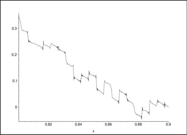
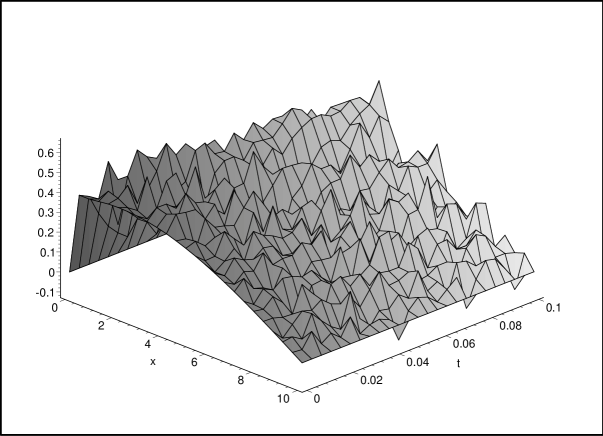
Although the discontinuity of the wave function vanishes for $t>0$, an infinite amount of energy continues to be stored in the potential well. This energy manifests itself in the form of a fractal wave function whose energy density in the well is everywhere infinite. The self-similar structure of the fractal wave function can be verified by plotting it on successively smaller intervals while at the same time increasing the number of terms in the Fourier series expansion. Fig. 4 shows the imaginary part of the wave function $\psi_{\chi}(x,t)$ at $t=10^{-17}$ seconds using a $50,000$-term Fourier series. The energy of the fractal wave function in Fig. 4 is infinite because the probability $p_{n}$ of finding the particle in the $n$th energy state decays like $p_{n}\sim n^{-2}$, while the $n$th energy level grows like $E_{n}\sim n^{2}$.

The fractal structure encountered here has been investigated previously by Berry (1996). Berry discussed the question of how a wave function in an infinite potential well evolves in time from a constant initial state $\psi(x,0)=1/\sqrt{L}$. Berry found that if an initial wave function in a potential well has a finite jump discontinuity so that it has infinite energy, then under unitary time evolution the wave function will instantly develop fractal structure. Other studies of fractal wave functions have been done by Wójcik et al. (2000), Berry et al. (2001) and references cited therein.

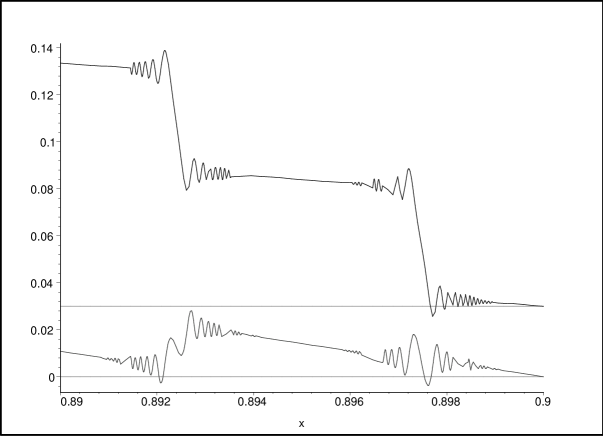
Although a fractal state such as (21) requires infinite energy to create, if we insert a barrier rapidly but in finite time and with finite energy, then the resulting wave function displays a fractal-like feature. However, because there is only finite energy, if a barrier is inserted in the vicinity of one end of the well, then for large $L$ it will take a while before the wave function at the other end of the well is excited. An example in which a barrier is inserted near one end of the well rapidly enough to excite the first one thousand energy levels is shown in Fig. 5, where we plot the imaginary part of the wave function in the vicinity of the other end of the well. As we see in Fig. 5, there is a time delay before the rise in the amplitude of the wave function near the well becomes noticeable.

Figure 5: Evolution of the imaginary part of the wave function. We set $L=10^{10}$Å and insert the barrier at $x_{0}=0.9\times 10^{10}$Å rapidly enough to excite the first $1,000$ energy levels. The plot displays the intervals $0\leq x\leq 0.1\times 10^{10}$ in units of Å and $10^{-3}\leq t\leq 10$ in units of seconds. The amplitude of the wave function in the vicinity of $x=0$ is exponentially small (of order $10^{-4}$) when $t\sim 10^{-3}$ seconds. Therefore, a force on the wall will not be detected at $x=0$ when $t\ll 1$.

7 Adiabatic insertion of an impenetrable barrier

Inserting an impenetrable barrier into a wave function at a nodeless point is similar to pushing an object through a viscous fluid. The work done in the process depends on the speed of insertion. In §6 we showed that it requires an infinite amount of work to insert the barrier instantaneously. However, a slow insertion of the barrier requires only a finite amount of work.

In this section we consider the case of an adiabatic (infinitely slow) insertion of a barrier at a nonnodal point $x_{0}$. Inserting a barrier creates a new node at $x_{0}$ and changes the state of the system. However, an adiabatic process is one in which the system does not depart from equilibrium. Thus, during an adiabatic insertion the change in the energy of the system is minimised.

We reconsider the configuration in §4, where a barrier was inserted into the initial state $\phi_{1}(x)$ at $x_{0}=L-\delta$. However, instead of an instantaneous insertion we now perform an adiabatic insertion. The states before and after the adiabatic insertion of the barrier are illustrated in Fig. 6, where we have taken $\delta=0.1\,L$. The final energy of the system is the sum of the ground-state energies on both sides of the inserted barrier, multiplied by the corresponding probability amplitudes. The energy required to insert the barrier is determined by the difference between the final and initial energies of the system:

$$\Delta E = \frac{\pi^{2}\hbar^{2}}{2m}\left(\frac{1}{(L-\delta)^{2}}\int_{0}^{L-\delta}\phi_{1}^{2}(x)\rd x+\frac{1}{\delta^{2}}\int_{L-\delta}^{1}\phi_{1}^{2}(x)\rd x-\frac{1}{L^{2}}\right)$$ (22)

$$= \frac{\pi^{2}\hbar^{2}}{2mL^{2}}\left(\frac{1}{\epsilon}+\frac{1}{1-\epsilon}+\frac{2\epsilon-1}{\pi\epsilon^{2}(1-\epsilon)^{2}}\sin(\pi\epsilon)\cos(\pi\epsilon)-1\right),$$

where $\epsilon=\delta/L$.

Figure 6: Adiabatic insertion of a barrier at $x_{0}=$0.9Å with $L=1$Å. The initial state $\phi_{1}(x)$ having support on $[0,1]$ becomes a pair of (unnormalised) ground states one on each side of the barrier.

For small $\epsilon$ the Taylor expansion of $\Delta E$ is

$$\Delta E\sim\frac{\pi^{2}\hbar^{2}}{2mL^{2}}\Big{(}2\epsilon+\mbox{$\textstyle\frac{2}{3}$}\pi^{2}\epsilon+3\epsilon^{2}+{\cal O}(\epsilon^{3})\Big{)}\quad(\epsilon\ll 1).$$ (23)

The term $\frac{2}{3}\pi^{2}\epsilon$ is a consequence of the cubic behaviour of the probability in (8) and is a feature of low-energy quantum states. High quantum number states do not have this term and thus this behaviour has no classical analogue.

What happens if we measure the presence or absence of the particle on one side of the inserted barrier, say, in $[L-\delta,L]$? If the particle is absent, then the energy that was contained in $[L-\delta,L]$ will be transferred to $[0,L-\delta]$, where the particle is now present. However, counter to the intuition one gains from Fig. 6, the Lüders state (the state having support on $[0,L-\delta]$ that results after the wave function collapses) is not a normalised ground state.

To show that the Lüders state is not the ground state we assume the contrary. If it were the ground state, then the final energy of the system would be proportional to $(L-\delta)^{-2}$. The initial energy of the system before the adiabatic insertion of the barrier was proportional to $L^{-2}$. The energy difference of these two ground states must equal the energy $\Delta E$ required to insert the barrier. However, the energy $\Delta E$ required to insert the barrier is greater than this difference except when the insertion is located at the centre $\delta=L/2$:

$$\frac{1}{(L-\delta)^{2}}\int_{0}^{L-\delta}\phi_{1}^{2}(x)\rd x+\frac{1}{\delta^{2}}\int_{L-\delta}^{1}\phi_{1}^{2}(x)\rd x-\frac{1}{L^{2}}\geq\frac{1}{(L-\delta)^{2}}-\frac{1}{L^{2}},$$ (24)

where equality holds only if $\delta=L/2$. Thus, the energy injected into the system by the adiabatic insertion of the barrier at $\delta\neq L/2$ is so large that after the absence of the particle on one side of the barrier is confirmed, the wave function on the other side will be excited to a state higher than the ground state.

For $\epsilon\ll 1$ the right side of (24) becomes

$$\frac{1}{(L-\delta)^{2}}-\frac{1}{L^{2}}\sim\frac{1}{L^{2}}\Big{(}2\epsilon+3\epsilon^{2}+{\cal O}(\epsilon^{3})\Big{)}.$$ (25)

This result shows that the term $\frac{2}{3}\pi^{2}\epsilon$ in (23) is the additional energy that excites the system above the ground state when the absence of the particle in the interval $[L-\delta,L]$ is confirmed. This additional term arises whenever we insert the barrier at a location away from the centre of the potential well that contains a low-energy initial wave function.

It is interesting to note that depending on whether a measurement to confirm the presence or absence of the particle in the region $[L-\delta,L]$ is conducted, the expectation value of the Hamiltonian in the region $[0,L-\delta]$ takes different values when $\epsilon\ll 1$. Specifically, if the system has not been disturbed by a measurement, then to first order in $\epsilon$ we have

$$\int_{0}^{L-\delta}\phi_{1}(x)H\phi_{1}(x)\rd x=\frac{\pi^{2}\hbar^{2}}{2mL^{2}}\big{(}1+2\epsilon\big{)}.$$ (26)

On the other hand, if the system has been disturbed by a measurement, then the energy expectation becomes

$${\rm tr}(\rho H)=\frac{\pi^{2}\hbar^{2}}{2mL^{2}}\Big{(}1+\left(2+\mbox{$\textstyle\frac{2}{3}$}\pi^{2}\right)\epsilon\Big{)}.$$ (27)

Here the density matrix $\rho$ reflects the two possible outcomes of the measurements, whose statistics is provided by (8). For example, for $\epsilon$ of order $1\%$ there is about a $6\%$ difference between the energy expectation values.

8 Maxwell’s daemon for square wells

A quantum version of Maxwell’s daemon was considered by numerous researchers (Zurek 1986, Bennett 1987, Lloyd 1997, and references therein). In the context of the square-well systems considered in this paper, the Maxwell daemon scenario is as follows: A barrier is inserted adiabatically at the centre of a well containing the initial ground-state wave function $\phi_{1}(x)$. A node appears at the centre, and on each side of the node the wave function is in the (unnormalised) ground state. The daemon then performs a measurement to determine on which side of the barrier the particle is present and in doing so causes the wave function to collapse. Until now, the barrier considered in this paper was fixed in place; however, in this scenario the barrier is a classical object that is allowed to slide to the left or right inside the well. The daemon then releases the barrier, and as the barrier slides and the subchamber containing the particle expands, energy is extracted from the collapsed wave function. This energy can be used to reduce the entropy of the environment. When the barrier reaches the edge of the well, the initial wave function is recovered. This appears to be a cyclic engine that violates the second law of thermodynamics.

The standard argument (see Landauer 1961 and Zurek 1986) to show why the second law is actually not violated is that to close the cycle of this engine completely the daemon must erase the information about where the particle was when the barrier was inserted. Because the probability of finding the particle in a given subchamber was $\frac{1}{2}$, the amount of this information is $\ln 2$. The act of erasing the memory balances the decrease in the entropy (the so-called Landauer’s principle) so that there is no violation of the second law.

If the barrier is not inserted at the centre of the well, the entropy associated with erasing the memory is reduced. This is because the probability of finding the particle in a given subchamber is not $\frac{1}{2}$. Classically, this reduced entropy still balances the reduction of the entropy in the environment. Similarly, for a quantum system in equilibrium with a high temperature heat reservoir, as considered by Zurek, Landauer’s erasure principle also applies without modification because no energy is needed to insert the barrier.

However, for small $\epsilon$ and for low-energy quantum states the entropy reduced in the environment no longer balances the information contained in the daemon’s memory. Specifically, the probabilities of trapping the particle in the subchambers are $p(\epsilon)$ and $1-p(\epsilon)$, where $p(\epsilon)$ is given in (8). The entropy lost by the daemon can be expressed as a series expansion for $\epsilon\ll 1$:

$$S(\epsilon)\sim\left[\mbox{$\textstyle\frac{2}{3}$}\pi^{2}\Big{(}1-\ln\left(\mbox{$\textstyle\frac{2}{3}$}\pi^{2}\right)\Big{)}-2\pi^{2}\ln(\epsilon)\right]\epsilon^{3},$$ (28)

which approaches zero rapidly as $\epsilon\to 0$. On the other hand, the energy that the daemon has extracted is of order $\epsilon$.

This apparent violation of the second law is avoided by recognising that inserting the barrier adiabatically at a nonnodal point requires a finite amount of work. Therefore, the usual explanation, which relies solely on Landauer’s principle, for why the second law is not violated is insufficient in such circumstances. We have shown here that Landauer’s principle when used in this quantum context must be augmented by including the energy required to insert the barrier.

9 Fractal states with unbounded entropy

Let us examine the entropy of fractal quantum states. The term entropy used here is the von Neumann entropy associated with the density matrix that represents the mixed state of the system after a measurement (of the energy, for example) is performed on the initial pure state. A pure state has zero entropy, so when we speak of the entropy of a fractal wave function, it is always understood to indicate the von Neumann entropy associated with the density matrix after energy measurement.

The fractal wave functions encountered here and elsewhere in the literature share the property that the associated entropy is finite. It is possible, however, to construct a special class of fractal wave functions whose entropies are infinite. To show that the entropy associated with states generated by an instantaneous insertion of the barrier is finite, we recall that the probability $p_{n}$ of finding the system in the $n$th energy level is given for large $n$ by $p_{n}\sim n^{-2}$. This follows directly from (11), and the same $n$-dependence applies to Berry’s fractal states (1996). Therefore, the von Neumann entropy $S=-\sum_{n}p_{n}\ln p_{n}$ is finite. In the case of fractal states considered by Wójcik et al. (2000), the probability $p_{n}$ decays exponentially fast, and thus the associated von Neumann entropy converges rapidly.

Figure 7: Evolution of the real part of the wave function (30), approximated by the first 10,000 terms in its Fourier expansion. We set $\nu=0.5$, $L=10$Å, and the mass of the particle is set to the mass $m_{\rm e}$ of an electron. The plot is given for the intervals $0\leq x\leq 10$ in units of Å and $0<t\leq 10^{-16}$ in units of seconds.

As noted above, we can create a new class of fractal wave functions for which the associated entropy is infinite. Consider as an example the probability

$$p_{n}=\frac{1/N(\nu)}{(n+\nu)[\ln(n+\nu)]^{2}},$$ (29)

where $\nu>0$ is a constant and $N(\nu)$ is the normalisation. The probability (29) is an example of a fat-tail distribution for which none of the associated moments exist and, similarly, the associated entropy is also infinite. The key idea here is that the norm of the state is finite because the integral $\int^{\Lambda}1/x(\ln x)^{2}\rd x=1/\ln\Lambda$ is finite as $\Lambda\to\infty$, while the entropy is infinite because the integral $\int^{\Lambda}1/x\ln x\,\rd x=\ln(\ln\Lambda)$ diverges as $\Lambda\to\infty$.

Letting $c_{n}=\sqrt{p_{n}}$, we can construct a wave function representing a state of a particle in the potential well:

$$\psi(x,t)=\sum_{n=1}^{\infty}\re^{-\ri E_{n}t/\hbar}c_{n}\phi_{n}(x).$$ (30)

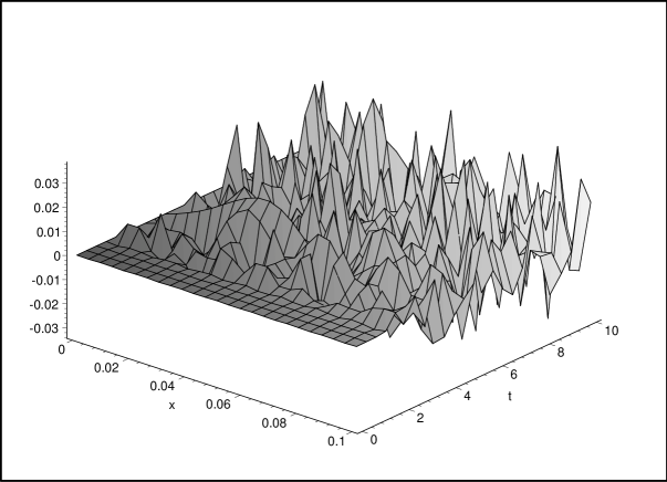
At $t=0$ this wave function is smooth for $x>0$ and singular at $x=0$. Such an initial state might be created by an instantaneous compression of the potential well at $x=0$. The key difference between the wave function (30) and the states considered in §6 is that at the boundary $x=0$ the initial wave function $\psi(x,0)$ (30) is infinite. However, once the system evolves in time, the wave function satisfies the homogeneous boundary condition at $x=0$ and becomes fractal. An example is displayed in Fig. 7.

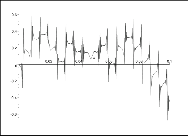
One particularly interesting characteristic behaviour associated with the wave function $\psi(x,t)$ of (30) is that whenever the time variable $t$ reaches the values

$$t=\frac{2kmL^{2}}{\pi^{2}\hbar}\quad(k=1,2,3,\ldots),$$ (31)

the wave function exhibits a peculiar ringing phenomenon as illustrated in Fig. 8. There are 117 oscillations of the kind shown in the figure in the interval $[0,L]$.

Figure 8: Ringing phenomenon of the wave function (30), approximated by the first 20,000 terms in its Fourier expansion. Whenever time reaches $t=2km_{\rm e}L^{2}/\pi^{2}\hbar$ $(k=1,2,3,\ldots)$, the wave function takes a characteristic form as shown here. We set $\nu=0.5$, $L=1$Å, and the plot is given for the interval $0\leq x\leq 0.1$ in units of Å, and time is set so that $\pi^{2}\hbar t/2m_{\rm e}L^{2}=1$ (about $10^{-15}$ seconds).

If we measure the energy of the system prescribed by the wave function (30), the entropy of the resulting mixed state is infinite even though the size $L$ of the system is finite. This seems to imply that quantum mechanics is not consistent with black hole physics, for which the entropy of a system is bounded by the surface area of a black hole (see Bekenstein 1994 and references cited therein). However, recall that the energy of the present system is also infinite. Thus, in order to create an infinite entropy state for a particle trapped in a potential well, the system must also possess infinite energy. One may argue that when the energy of the system reaches a threshold value, the system collapses to form a black hole. As a consequence, the entropy of the system cannot diverge. On the other hand, there are other systems, such as the bound states of a hydrogen atom, for which energy expectation is always finite. In §10 we examine some other quantum systems having unbounded entropy.

10 Limits on quantum states having infinite entropy

One can construct wave functions using the probability weights (29) for other quantum systems, such as a harmonic oscillator or a hydrogen atom. What can we say about the energy and size of such systems?

We investigate first the properties of a particle trapped in a harmonic potential $V(x)=\frac{1}{2}m\omega^{2}x^{2}$. The eigenstates of the Hamiltonian (with $m\omega/\hbar=1$) are

$$\phi_{n}(x)=\frac{\pi^{1/4}}{\sqrt{2^{n}n!}}\re^{-\frac{1}{2}x^{2}}H_{n}(x),$$ (32)

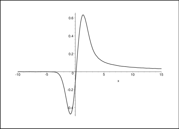
where $H_{n}(x)$ denotes the $n$th Hermite polynomial. Using these eigenstates we construct an initial wave function $\psi(x)=\sum_{n}c_{n}\phi_{n}(x)$.

Unlike the case of a particle in a square well, the wave function $\psi(x)$ exhibits no discontinuity or fractal structure, as is evident from the plot of the wave function in Fig. 9. This is because the initial wave function $\psi(x)$ does not violate the boundary conditions associated with the Schrödinger eigenvalue problem. Nonetheless, if an energy measurement is performed on the system prepared in the state $\psi(x)$, the resulting density matrix has infinite von Neumann entropy. Similarly, the energy of the system is also infinite because the expectation value of the Hamiltonian diverges. The energy expectation value can be determined either by taking the sum $\sum_{n}p_{n}E_{n}$, where $E_{n}\sim n$ ($n\to\infty$), or by considering the asymptotic behaviour of the wave function $\psi(x)$. Specifically, numerical studies indicate that

$$\psi(x)\sim\frac{0.44}{\sqrt{x}\ln x}$$ (33)

as $x\to\infty$. Therefore, the probability distribution $\psi^{2}(x)$ associated with the position of the particle has a fat tail and none of the moments exists. In particular, the expectation value of $x$ is infinite, so the characteristic size of the system is infinite.

Figure 9: Initial wave function $\psi(x)$ constructed from the weights (29) and the eigenstates (32). The wave function is smooth and square integrable. However, its square $\psi^{2}(x)$ possesses a fat-tail distribution. Asymptotically, we have $\psi(x)\sim(\sqrt{x}\ln x)^{-1}$ as $x\to+\infty$.

Let us now consider the case of a Coulomb potential for which the energy eigenvalues $E_{n}$ are proportional to $-1/n$. In this case, the expectation value of the Hamiltonian is necessarily bounded for an arbitrary state. Therefore, it is possible to create a mixed state using bound states of the hydrogen atom for which the entropy is infinite, while keeping the system energy finite. However, the expectation value of $r$ in the $n$th Coulombic bound state grows like $n^{2}$ for large $n$ (Messiah 1958). Therefore, the expectation value of the radius $r$ in the infinite-entropy state is infinite. Hence, the surface area of the mixed state with diagonal elements $p_{n}$ given by (29), is infinite.

With these observations we conjecture that for a quantum state to have infinite entropy, either its energy or size, or possibly both, must also diverge. If this indeed is the case, then we may argue that quantum theory is not in direct contradiction with laws of black hole thermodynamics.

11 Effects of separating the subchambers

Can the nonlocality property of quantum mechanics described in this paper be used to communicate rapidly over great distances? Recall that diffusion is a spreading process that proceeds infinitely fast. The Schrödinger equation is a diffusion equation, so an initial wave function having compact support will evolve immediately into a wave function that is nonvanishing over all space. Nevertheless, at great distances the wave function is exponentially small, and it is impossible to take advantage of the nonlocality of the diffusion process to send signals.

However, if the support of the wave function remains finite, one may ask if instantaneous communication now becomes practical: Can we use the configuration of two widely separated square wells and the entanglement of states to transmit signals instantaneously?

Suppose we prepare many identical copies of a system of a single particle trapped in a square well and insert impenetrable barriers into each of the potential wells. One subregion is taken to observer $A$ and the other taken to observer $B$. This establishes a ‘telephone line’ (cf. Gisin 1990) between $A$ and $B$. Suppose that at an agreed time $A$ wishes to transmit one bit information to $B$. To do so $A$ will either measure the presence of the particles or $A$ will do nothing. If observer $B$ can determine statistically whether $A$ has performed the measurement, then one bit of information is transmitted.

Considerations of such a problem require careful analysis of the effects of the physical displacement of the subchambers on the wave functions contained therein. If the subchambers are separated adiabatically, then by definition this separation will not affect the wave functions. However, such a separation requires an infinite amount of time. As a consequence, even if an instantaneous communication across long distances were possible (for example, using the discrepancy of the energy expectations in (26) and (27)), it requires an infinite amount of time to establish the telephone line.

To overcome this problem we could try to separate the boxes in finite time. However, in this case we believe that the wave function collapses to a density matrix because accelerating the box constitutes a measurement of whether there is a particle in the box. If it were possible to separate the boxes in a finite time without collapsing the wave function, then it would be possible to send signals instantaneously over great distances. Moreover, since the accelerated box can extract energy from its environment, it is possible to transmit an arbitrarily large quantity of energy instantaneously across large distances.

12 Discussion

The system considered here is perhaps the simplest quantum system represented in terms of an infinite-dimensional Hilbert space. Nevertheless, by a thorough analysis of the various effects of dividing the system into a pair of subsystems we were led to a number of interesting and peculiar features of quantum mechanics. Some of the gedanken experiments considered in this paper might well be feasible using the procedures recently developed by Konstantinov and Maris (2003).

Because an insertion of the barrier in a potential well creates entangled subsystems, one may ask whether it is possible to formulate a version of the Bell inequality that is appropriate for this configuration. The Bell inequality relies on the statistics of noncommuting observables. In the present example one might consider the measurement of the presence or absence of a particle in a subchamber and the energy contained in a subchamber as the relevant observables.

In the discussion of a quantum-mechanical Maxwell daemon we found an example in which the standard argument based on Landauer’s principle is insufficient. Nonetheless, we were able to resolve the problem by taking into account the energy needed to insert the barrier into the potential well.

We have found a new class of fractal states having infinite entropy. Our discussion in §10 suggests that if a quantum state has infinite entropy, then it must also have infinite energy and/or infinite size. This raises the interesting question of whether it is possible to derive a bound on entropy or perhaps even a bound on the gravitational constant, conditional on finite size and energy, in the context of nonrelativistic quantum mechanics.

The discussion in §11 concerning the mechanical displacement and separation of the subchambers leads to an interesting gedanken experiment to test the so-called Wigner interpretation of quantum mechanics. According to this interpretation, the collapse of the wave function occurs only when the result of a measurement has been registered by a conscious being (Wigner 1963). Therefore, if the subchambers are displaced by a mechanical device that does not involve conscious awareness, and as a result the wave function does not collapse, then it is theoretically possible to transport an unbounded quantity of energy instantaneously over large distances.