The non-Markovian quantum behavior of open systems: An exact Monte Carlo method employing stochastic product states

Abstract

It is shown that the exact dynamics of a composite quantum system can be represented through a pair of product states which evolve according to a Markovian random jump process. This representation is used to design a general Monte Carlo wave function method that enables the stochastic treatment of the full non-Markovian behavior of open quantum systems. Numerical simulations are carried out which demonstrate that the method is applicable to open systems strongly coupled to a bosonic reservoir, as well as to the interaction with a spin bath. Full details of the simulation algorithms are given, together with an investigation of the dynamics of fluctuations. Several potential generalizations of the method are outlined.

I Introduction

A great deal of the dynamics of open systems can be described, to a reasonable degree of accuracy, by Markovian quantum master equations. Important examples are given by the weak-coupling interaction of radiation with matter in atomic physics and quantum optics COHEN ; GARDINER . However, non-Markovian quantum dynamics NAKAJIMA ; ZWANZIG ; FEYNMAN ; LEGGETT is known to play a significant role in many applications of the theory of open quantum systems TheWork currently under discussion in the literature, e.g. the dynamics of the atom laser SAVAGE , environment-induced decoherence at low temperatures (for an example, see DECOHERENCE ), and quantum devices interacting with a spin bath STAMP .

Quantum Monte Carlo techniques have been shown to provide efficient numerical tools for the treatment of the dynamics of open systems in the Markovian regime SWFM . In these techniques one constructs a stochastic dynamics for the open system’s state vector $\psi(t)$ such that the reduced density matrix $\rho_{S}(t)$ of the open system is recovered through the expression $\rho_{S}(t)={\mathrm{E}}(|\psi(t)\rangle\langle\psi(t)|)$, where ${\mathrm{E}}$ denotes the expectation value or ensemble average of the underlying process. This is the standard Monte Carlo wave function method which has been widely used in many physical problems of quantum optics and condensed matter theory.

The idea of the Monte Carlo wave function method can be extended to the treatment of non-Markovian quantum processes which cannot be described by a Markovian quantum master equation. One such method DGS is based on a stochastic integro-differential equation for the wave function involving a non-local retarded memory kernel. The solution of non-local equations of motion can be circumvented by employing a pair $\psi_{1}(t)$, $\psi_{2}(t)$ of random wave functions of the open system and by expressing the reduced density matrix with the help of the mean value $\rho_{S}(t)={\mathrm{E}}(|\psi_{1}(t)\rangle\langle\psi_{2}(t)|)$ BKP . This method of propagating a pair of wave functions requires the construction of an appropriate time-local non-Markovian master equation. Such an equation can be obtained with the help of the time-convolutionless (TCL) projection operator technique which leads to a systematic perturbation expansion for the time-dependent generator of the master equation. However, for strong system-environment couplings calculations based on the TCL expansion become extremely complicated and the derivation of an appropriate TCL generator of high order is, in general, not feasible in practice. A further possibility is to use an explicit expression for the influence functional of the open system to obtain stochastic differential equations for a pair of random wave functions STOCK . This method is, however, restricted to Gaussian reservoirs and linear dissipation.

In this paper the details of a new method proposed in PDP-SHORT are presented, which allows to attack the problem of non-Markovian quantum evolution by means of a Monte Carlo wave function technique. The basic idea is to introduce a pair $|\Phi_{1}(t)\rangle$, $|\Phi_{2}(t)\rangle$ of random states of the total system, with the aim of a stochastic formulation of the exact von Neumann dynamics of the composite system. A similar idea has been used recently to construct an exact diffusion process for a pair of one-particle wave functions describing systems of identical Bosons CARUSO1 and Fermions CHOMAZ . Here, the state vector dynamics is assumed to represent a piecewise deterministic process (PDP). This is a Markovian jump process with smooth, deterministic evolution periods between successive jumps. The stochastic states of the total system are supposed to be tensor product states of the form $|\Phi_{1}\rangle=\psi_{1}\otimes\chi_{1}$ and $|\Phi_{2}\rangle=\psi_{2}\otimes\chi_{2}$. The method thus involves four stochastic state vectors, namely a pair $\psi_{1}$, $\psi_{2}$ of state vectors of the open system, and a pair $\chi_{1}$, $\chi_{2}$ of state vectors of the environment. The open system’s reduced density matrix can then be represented in terms of the expectation value

$$\rho_{S}(t)={\mathrm{E}}\left(|\psi_{1}(t)\rangle\langle\psi_{2}(t)|\langle\chi_{2}(t)|\chi_{1}(t)\rangle\right).$$ (1)

Contrary to the standard methods mentioned above, this representation employs an average over the product of two quantities: The dyadic $|\psi_{1}\rangle\langle\psi_{2}|$ of a pair of state vectors of the open system, and the scalar product $\langle\chi_{2}|\chi_{1}\rangle$ of a corresponding pair of environment states. It will be shown that this representation allows to design a Markovian stochastic process which unravels the full non-Markovian behavior of the reduced density matrix.

The paper is structured as follows. Section II contains the general construction of the PDP representing the exact von Neumann dynamics of the composite system, an investigation of the dynamics of the fluctuations of the stochastic process, as well as a detailed description of the Monte Carlo algorithm of the open system dynamics. The example of the non-perturbative decay of a two-state system into a bosonic reservoir is discussed in Sec. III. This section contains numerical simulations of the non-Markovian dynamics of the decay into a reservoir in the regime of strong couplings and corresponding long memory times. The quantum dynamics of a specific spin bath model is investigated in Sec. IV. This model describes the interaction of a single electron spin in a quantum dot with an external magnetic field and a bath of nuclear spins. Section V contains the conclusions and indicates various potential generalizations of the stochastic method.

II General formulation of the method

II.1 Construction of the PDP

We investigate the general situation of an open system with underlying Hilbert space ${\mathcal{H}}_{S}$, which is coupled to an environment with Hilbert space ${\mathcal{H}}_{E}$. The state space of the composite, total quantum system is given by the tensor product ${\mathcal{H}}_{S}\otimes{\mathcal{H}}_{E}$. Working in the interaction picture we write the Hamiltonian describing the system-environment interaction as

$$H_{I}(t)=\sum_{\alpha}A_{\alpha}(t)\otimes B_{\alpha}(t).$$ (2)

The $A_{\alpha}(t)$ and the $B_{\alpha}(t)$ are interaction picture operators acting in ${\mathcal{H}}_{S}$ and ${\mathcal{H}}_{E}$, respectively. The evolution of the density matrix $\rho(t)$ of the total system is then governed by the von Neumann equation ($\hbar=1$),

$$\frac{d}{dt}\rho(t)=-i[H_{I}(t),\rho(t)].$$ (3)

Our central goal is to construct a representation of $\rho(t)$ in terms of the expectation value

$$\rho(t)={\rm{E}}(|\Phi_{1}(t)\rangle\langle\Phi_{2}(t)|),$$ (4)

which is determined through a pair $|\Phi_{1}(t)\rangle$, $|\Phi_{2}(t)\rangle$ of stochastic state vectors of the composite quantum system. Equivalently, one may define the quantity

$$R(t)=|\Phi_{1}(t)\rangle\langle\Phi_{2}(t)|,$$ (5)

which is a random operator on ${\mathcal{H}}_{S}\otimes{\mathcal{H}}_{E}$, and write the density matrix as the mean value of this operator, that is $\rho(t)={\rm{E}}(R(t))$.

In the following we suppose that the stochastic state vectors $|\Phi_{\nu}(t)\rangle$ ($\nu=1,2$) introduced in Eq. (4) are direct products of certain system states $\psi_{\nu}(t)\in{\mathcal{H}}_{S}$ and environment states $\chi_{\nu}(t)\in{\mathcal{H}}_{E}$, that is we have

$$|\Phi_{\nu}(t)\rangle=\psi_{\nu}(t)\otimes\chi_{\nu}(t),\qquad\nu=1,2.$$ (6)

The reduced density matrix $\rho_{S}(t)$ of the open system is defined through the partial trace over the variables of the environment, $\rho_{S}(t)={\mathrm{tr}}_{E}\rho(t)$. In view of Eqs. (4) and (6) this definition immediately leads to the relation (1).

It is important to realize that a representation of the form given in Eqs. (4) and (6) is possible for any initial state $\rho(t=0)$. This means that any given density matrix $\rho\equiv\rho(0)$ of the composite quantum system can be written as the mean value $\rho={\rm{E}}(|\Phi_{1}\rangle\langle\Phi_{2}|)$, in which the random states $|\Phi_{\nu}\rangle$ are direct products of the form (6). In particular, it is not necessary to demand that $\rho$ describes an initial state without system-environment correlations.

A formal proof of this statement may be carried out as follows. One first observes that a sequence of pairs $(|\Phi_{1}^{\lambda}\rangle,|\Phi_{2}^{\lambda}\rangle)$ of state vectors, which occur with corresponding probabilities $p_{\lambda}$, gives rise to the expectation value

$$\rho={\rm{E}}(|\Phi_{1}\rangle\langle\Phi_{2}|)=\sum_{\lambda}p_{\lambda}|\Phi^{\lambda}_{1}\rangle\langle\Phi^{\lambda}_{2}|.$$ (7)

Of course, $p_{\lambda}$ provides a probability distribution satisfying $p_{\lambda}\geq 0$ and $\sum_{\lambda}p_{\lambda}=1$. Introducing new states through the relation $|\Psi_{\nu}^{\lambda}\rangle=\sqrt{p_{\lambda}}|\Phi_{\nu}^{\lambda}\rangle$, we can write

$$\rho=\sum_{\lambda}|\Psi^{\lambda}_{1}\rangle\langle\Psi^{\lambda}_{2}|.$$ (8)

Thus, to prove the above statement we have to show that any given density matrix $\rho$ of the composite quantum system can be brought into the form (8), whereby the $|\Psi^{\lambda}_{\nu}\rangle$ must be direct products. To demonstrate that this is in fact possible we introduce an ON-basis $\{\psi_{i}\}$ in ${\mathcal{H}}_{S}$ and an ON-basis $\{\chi_{n}\}$ in ${\mathcal{H}}_{E}$ and write the given $\rho$ as follows,

$$\rho=\sum_{ijnm}\rho_{ijnm}|\psi_{i}\rangle\langle\psi_{j}|\otimes|\chi_{n}\rangle\langle\chi_{m}|,$$ (9)

where

$$\rho_{ijnm}\equiv\langle\psi_{i}\chi_{n}|\rho|\psi_{j}\chi_{m}\rangle\equiv|\rho_{ijnm}|e^{2i\varphi_{ijnm}}.$$

Next, one introduces a collective index $\lambda=(ijnm)$ and defines the states

$$|\Psi^{\lambda}_{1}\rangle = \sqrt{|\rho_{ijnm}|}e^{+i\varphi_{ijnm}}\psi_{i}\otimes\chi_{n},$$ (10)

$$|\Psi^{\lambda}_{2}\rangle = \sqrt{|\rho_{ijnm}|}e^{-i\varphi_{ijnm}}\psi_{j}\otimes\chi_{m},$$ (11)

which allow one to write Eq. (9) in the desired form (8). This completes the proof since the states (10) and (11) are indeed direct products.

The aim is now to construct an appropriate stochastic process for the state vectors $|\Phi_{\nu}(t)\rangle$ which exactly reproduces the von Neumann equation (3) through the expectation value (4). As mentioned in the Introduction we suppose that the time-evolution represents a piecewise deterministic process (PDP). A convenient way of formulating a PDP is to write stochastic differential equations for the random variables. The foundations of the calculus of PDPs and its applications to the quantum theory of open systems may be found in TheWork . In view of the representation (6) the stochastic dynamics can be defined in terms of stochastic differential equations for the state vectors $\psi_{\nu}(t)$ and $\chi_{\nu}(t)$,

$$d\psi_{\nu}(t) = F_{\nu}dt+dJ_{\nu},$$ (12)

$$d\chi_{\nu}(t) = G_{\nu}dt+dK_{\nu}.$$ (13)

These equations reflect the general structure of a PDP: The terms $F_{\nu}dt$ and $G_{\nu}dt$ represent the deterministic evolution periods, the drift of the process, while the terms $dJ_{\nu}$ and $dK_{\nu}$ provide the contributions from the random, instantaneous jumps of the process. These jump contributions are taken to be of the form

$$dJ_{\nu} = \sum_{\alpha}\left(-iL_{\alpha\nu}A_{\alpha}-I\right)\psi_{\nu}dN_{\alpha\nu}(t),$$ (14)

$$dK_{\nu} = \sum_{\alpha}\left(M_{\alpha\nu}B_{\alpha}-I\right)\chi_{\nu}dN_{\alpha\nu}(t).$$ (15)

Here, $I$ denotes the identity operator and $L_{\alpha\nu}$, $M_{\alpha\nu}$ are c-number functionals which will be specified below. The quantities $dN_{\alpha\nu}(t)$ are known as Poisson increments. They are independent, random numbers which take on the possible values $0$ or $1$ and satisfy the relation

$$dN_{\alpha\nu}(t)dN_{\beta\mu}(t)=\delta_{\alpha\beta}\delta_{\nu\mu}dN_{\alpha\nu}(t).$$ (16)

Under the condition that $dN_{\alpha\nu}(t)=1$ for a particular $\alpha$ and $\nu$ the other Poisson increments therefore vanish and, by virtue of the Eqs. (14) and (15), the state vectors then carry out the instantaneous jumps

$$\psi_{\nu}\longrightarrow-iL_{\alpha\nu}A_{\alpha}\psi_{\nu},\qquad\chi_{\nu}\longrightarrow M_{\alpha\nu}B_{\alpha}\chi_{\nu}.$$ (17)

The expectation values of the Poisson increments are given by

$${\mathrm{E}}(dN_{\alpha\nu}(t))=\Gamma_{\alpha\nu}dt.$$ (18)

This implies that $dN_{\alpha\nu}(t)=1$ with probability $\Gamma_{\alpha\nu}dt$ and, hence, the jumps (17) occur at a rate $\Gamma_{\alpha\nu}$, which will also be determined below. If, on the other hand, all Poisson increments vanish we have $d\psi_{\nu}(t)=F_{\nu}dt$ and $d\chi_{\nu}(t)=G_{\nu}dt$, which means that the state vectors follow the deterministic drift during $dt$.

Our next step consists in deriving a stochastic equation for the random operator $R(t)$ defined in Eq. (5), which will then lead to an equation of motion for the expectation value (4). Employing the calculus of PDPs one finds

$$dR=|d\Phi_{1}\rangle\langle\Phi_{2}|+|\Phi_{1}\rangle\langle d\Phi_{2}|+|d\Phi_{1}\rangle\langle d\Phi_{2}|.$$

The third term on the right-hand side of this equation involves the products $dN_{\alpha 1}dN_{\beta 2}$ of the Poisson increments, which vanish by virtue of Eq. (16). This means that the state vectors $|\Phi_{1}(t)\rangle$ and $|\Phi_{2}(t)\rangle$ evolve independently and that we may write

$$dR=|d\Phi_{1}\rangle\langle\Phi_{2}|+|\Phi_{1}\rangle\langle d\Phi_{2}|.$$ (19)

With the help of the stochastic differential equations (12) and (13) the state vector increments are found to be

$$|d\Phi_{\nu}\rangle = d\psi_{\nu}\otimes\chi_{\nu}+\psi_{\nu}\otimes d\chi_{\nu}+d\psi_{\nu}\otimes d\chi_{\nu}$$

$$= (F_{\nu}dt+dJ_{\nu})\otimes\chi_{\nu}+\psi_{\nu}\otimes(G_{\nu}dt+dK_{\nu})$$

$$+dJ_{\nu}\otimes dK_{\nu}.$$

On using the structure of the jump terms (14) and (15) and relation (16) the third term may be written

$$dJ_{\nu}\otimes dK_{\nu} = \sum_{\alpha}\left(-iL_{\alpha\nu}A_{\alpha}-I\right)\psi_{\nu}$$

$$\qquad\otimes\left(M_{\alpha\nu}B_{\alpha}-I\right)\chi_{\nu}dN_{\alpha\nu}$$

$$= -dJ_{\nu}\otimes\chi_{\nu}$$

$$+\sum_{\alpha}\left(-iL_{\alpha\nu}A_{\alpha}-I\right)\psi_{\nu}$$

$$\qquad\otimes M_{\alpha\nu}B_{\alpha}\chi_{\nu}dN_{\alpha\nu},$$

which leads to

$$|d\Phi_{\nu}\rangle = F_{\nu}dt\otimes\chi_{\nu}$$

$$+\psi_{\nu}\otimes\left(G_{\nu}dt-\sum_{\alpha}dN_{\alpha\nu}\chi_{\nu}\right)$$

$$-i\sum_{\alpha}L_{\alpha\nu}M_{\alpha\nu}(A_{\alpha}\psi_{\nu})\otimes(B_{\alpha}\chi_{\nu})dN_{\alpha\nu}.$$

This equation provides an exact relation for the stochastic increments $|d\Phi_{\nu}\rangle$. To ensure that the first and the second term on the right-hand side vanish when taking the average over the Poisson increments, we now set

$$F_{\nu}\equiv 0,\qquad G_{\nu}\equiv\Gamma_{\nu}\chi_{\nu},$$ (21)

where

$$\Gamma_{\nu}\equiv\sum_{\alpha}\Gamma_{\alpha\nu},$$ (22)

and

$$\Gamma_{\alpha\nu}\equiv\frac{1}{L_{\alpha\nu}M_{\alpha\nu}}.$$ (23)

This yields the expression

$$|d\Phi_{\nu}\rangle = \psi_{\nu}\otimes\left(\Gamma_{\nu}dt-\sum_{\alpha}dN_{\alpha\nu}\right)\chi_{\nu}$$

$$-i\sum_{\alpha}\Gamma^{-1}_{\alpha\nu}(A_{\alpha}\psi_{\nu})\otimes(B_{\alpha}\chi_{\nu})dN_{\alpha\nu}.$$

Finally, we substitute (II.1) into (19) to arrive at

$$dR(t)=-i[H_{I}(t),R(t)]dt+dS(t).$$ (25)

Equation (25) is the desired exact stochastic equation of motion of the random operator $R(t)$. The drift term involves the commutator with the interaction Hamiltonian $H_{I}(t)$, while the noise term is given by the stochastic increment

$$dS(t)=dT_{1}R(t)+R(t)dT_{2}^{\dagger},$$ (26)

with

$$dT_{\nu}=\sum_{\alpha}\left(\Gamma_{\alpha\nu}dt-dN_{\alpha\nu}\right)\left(I+i\Gamma^{-1}_{\alpha\nu}A_{\alpha}B_{\alpha}\right).$$ (27)

According to Eqs. (18) and (27) the average over the Poisson increments yields ${\mathrm{E}}(dT_{\nu})=0$. By virtue of Eq. (26) this gives ${\mathrm{E}}(dS)=0$. Thus, if we take the average of both sides of Eq. (25) we are led directly to the von Neumann equation (3). This shows that on average the stochastic dynamics defined by the differential equations (12) and (13) indeed reproduces the exact von Neumann dynamics of the density matrix of the combined system. We have thus achieved the goal of constructing a stochastic formulation of the evolution of the total system by means of a Markovian piecewise deterministic process.

Up to this point the quantities $L_{\alpha\nu}$ and $M_{\alpha\nu}$ are completely arbitrary with the only restriction that $\Gamma_{\alpha\nu}\geq 0$ (see Eq. (23)), which guarantees that the expectation values ${\mathrm{E}}(dN_{\alpha\nu})$ are positive, as it should be for random Poisson increments (see Eq. (18)). In the following we choose

$$L_{\alpha\nu}=\frac{||\psi_{\nu}||}{||A_{\alpha}\psi_{\nu}||},\qquad M_{\alpha\nu}=\frac{||\chi_{\nu}||}{||B_{\alpha}\chi_{\nu}||}.$$ (28)

The advantage of this choice is that the jumps described by Eq. (17) then conserve the norm of the stochastic state vectors $\psi_{\nu}$ and $\chi_{\nu}$. Summarizing, the stochastic differential equations defining the PDP now read as follows,

$$d\psi_{\nu} = \sum_{\alpha}\left(\frac{-i||\psi_{\nu}||}{||A_{\alpha}\psi_{\nu}||}A_{\alpha}-I\right)\psi_{\nu}dN_{\alpha\nu}(t),$$ (29)

$$d\chi_{\nu} = \Gamma_{\nu}\chi_{\nu}dt$$ (30)

$$+\sum_{\alpha}\left(\frac{||\chi_{\nu}||}{||B_{\alpha}\chi_{\nu}||}B_{\alpha}-I\right)\chi_{\nu}dN_{\alpha\nu}(t),$$

where $\Gamma_{\nu}$ is given by Eq. (22) and by

$$\Gamma_{\alpha\nu}=\frac{||A_{\alpha}\psi_{\nu}||\cdot||B_{\alpha}\chi_{\nu}||}{||\psi_{\nu}||\cdot||\chi_{\nu}||}.$$ (31)

We observe that $\psi_{\nu}(t)$ is a pure, norm-conserving jump process, while $\chi_{\nu}(t)$ is a PDP with norm-conserving jumps and a linear drift which leads to a monotonic increase of the norm of $\chi_{\nu}$.

II.2 Dynamics of fluctuations

As a measure of the size of the fluctuations of the stochastic process constructed above we define CARUSO1

$$D^{2}(t) \equiv {\mathrm{E}}\left(||R(t)-\rho(t)||^{2}\right)$$ (32)

$$= {\mathrm{E}}\left({\mathrm{tr}}\left\{\left[R(t)-\rho(t)\right]^{\dagger}\left[R(t)-\rho(t)\right]\right\}\right).$$

The quantity $D(t)$ is thus the root mean square distance from the stochastic operator $R(t)$ to its mean value $\rho(t)={\mathrm{E}}(R(t))$, the distance being determined through the Hilbert-Schmidt norm $||A||=\sqrt{\mathrm{tr}\{A^{\dagger}A\}}$, where the trace is taken over the Hilbert space of the total system. Equation (32) may be written as

$$D^{2}(t)={\mathrm{E}}\left({\mathrm{tr}}\left\{R^{\dagger}(t)R(t)\right\}\right)-{\mathrm{tr}}\rho^{2}(t).$$ (33)

Since the dynamics of $\rho(t)$ represents a unitary transformation the trace over the square of $\rho(t)$ is constant in time. For a pure initial state $\rho(0)$ we have ${\mathrm{tr}}\rho^{2}\equiv 1$. Moreover, in the case of a sharp initial state, that is for $R(0)=\rho(0)$, one finds that $D^{2}(0)=0$.

Our aim is to estimate the size of the fluctuations. To this end we first derive a differential equation for the mean square distance $D^{2}(t)$. With the help of the stochastic equation of motion (25) and of definition (26) the differential of $D^{2}(t)$ is found to be

$$dD^{2} = {\mathrm{E}}\left({\mathrm{tr}}\left\{dS^{\dagger}dS\right\}\right)$$ (34)

$$= {\mathrm{E}}\left({\mathrm{tr}}\left\{dT_{1}^{\dagger}dT_{1}RR^{\dagger}+dT_{2}^{\dagger}dT_{2}R^{\dagger}R\right\}\right).$$

Using then the definition (27) of the quantities $dT_{\nu}$ as well as Eqs. (5), (16) and (18), we obtain

$$\frac{dD^{2}}{dt}={\mathrm{E}}\left(\sum_{\alpha\nu}\Gamma_{\alpha\nu}\frac{||\left(I+i\Gamma_{\alpha\nu}^{-1}A_{\alpha}B_{\alpha}\right)|\Phi_{\nu}\rangle||^{2}}{||\,|\Phi_{\nu}\rangle||^{2}}{\mathrm{tr}}\left\{R^{\dagger}R\right\}\right)\!\!.$$

The choice (28) finally yields

$$\frac{dD^{2}}{dt}=2{\mathrm{E}}\left(\sum_{\nu}\Gamma_{\nu}{\mathrm{tr}}\left\{R^{\dagger}R\right\}\right).$$ (35)

Equation (35) is an exact differential equation for the fluctuations of the random process. To find a rough estimate of the size of the fluctuations we suppose that the rates $\Gamma_{\nu}$ are bounded from above, that is $\Gamma_{\nu}\leq\Gamma_{0}$. This leads to the inequality

$$\frac{dD^{2}}{dt}\leq 4\Gamma_{0}\left(D^{2}+{\mathrm{tr}}\rho^{2}\right),$$ (36)

which, on integrating, gives

$$D^{2}(t)\leq\left({\mathrm{tr}}\rho^{2}\right)\left(e^{4\Gamma_{0}t}-1\right)+D^{2}(0)e^{4\Gamma_{0}t}.$$ (37)

This inequality provides a strict upper bound of the fluctuations of the random process. We note that the right-hand side of (37) is finite for any finite time $t$. This leads to the important conclusion that the fluctuations of the process are finite for all finite times.

Let us discuss in more detail the case of a sharp initial state, that is $D^{2}(0)=0$. We observe that for small times satisfying $4\Gamma_{0}t\ll 1$ the root mean square distance then increases at most as the square root of time,

$$D(t)\leq\sqrt{({\mathrm{tr}}\rho^{2})4\Gamma_{0}t}.$$ (38)

For large times, $4\Gamma_{0}t\gg 1$, the root mean square distance may increase, however, exponentially with time,

$$D(t)\leq\sqrt{{\mathrm{tr}}\rho^{2}}e^{2\Gamma_{0}t}.$$ (39)

This shows that the stochastic method is useful for short and intermediate times, where the relevant time scale is given by $1/2\Gamma_{0}$. One further expects that the method is, in general, not efficient numerically for times which are large compared to $1/2\Gamma_{0}$, because of a possible exponential increase of the fluctuations in this regime. It must be emphasized, however, that the statistical errors can be reduced considerably by employing the statistical independence of the increments $|d\Phi_{\nu}\rangle$ (see Sec. II.3.2), or by using a more complicated ansatz for the structure of the stochastic states (see Sec. V). It should also be noted that the statistical errors are often much smaller than the upper bound given in the inequality (39). An example will be discussed in Sec. IV.2.

II.3 The stochastic simulation method

II.3.1 Numerical algorithm

The stochastic simulation method consists in a numerical Monte Carlo simulation of the stochastic differential equations (29) and (30). A realizations $\psi_{\nu}(t)$, $\chi_{\nu}(t)$ of the process can be generated by means of the following algorithm.

1. Suppose that the last jump into states $\psi_{\nu}(t)$, $\chi_{\nu}(t)$ occurred at some time $t$. In the case that $t$ is the initial time $t=0$, these states are taken to be the initial states which must be drawn from the probability distribution representing the initial density matrix through $\rho(0)={\mathrm{E}}(R(0))$.

2. The next jump takes place at time $t+\tau$, where the $\tau$ is a stochastic time step, the random waiting time, which is to be determined from the cumulative waiting time distribution function

$$F(\tau)=1-\exp\left(-\int_{t}^{t+\tau}ds\Gamma_{\nu}(s)\right).$$ (40)

A random number $\tau$ following this distribution can be generated, for example, by drawing a uniform random number $\eta\in(0,1)$ and by solving the equation

$$\eta=\exp\left(-\int_{t}^{t+\tau}ds\Gamma_{\nu}(s)\right)$$ (41)

for $\tau$. In between the previous and the next jump, that is within the time interval $[t,t+\tau]$ the realization follows the deterministic drift which is given by

$$\psi_{\nu}(t^{\prime}) = \psi_{\nu}(t),$$ (42)

$$\chi_{\nu}(t^{\prime}) = \chi_{\nu}(t)\exp\left(\int_{t}^{t^{\prime}}ds\Gamma_{\nu}(s)\right),$$ (43)

where $t\leq t^{\prime}\leq t+\tau$.

3. Select a particular jump, that is select a particular value of the index $\alpha$ with probability

$$p_{\alpha\nu}=\frac{\Gamma_{\alpha\nu}(t+\tau)}{\sum_{\alpha}\Gamma_{\alpha\nu}(t+\tau)}.$$ (44)

The corresponding jumps of the state vectors at time $t+\tau$ then amount to the replacements

$$\psi_{\nu} \longrightarrow \frac{-i||\psi_{\nu}||}{||A_{\alpha}\psi_{\nu}||}A_{\alpha}\psi_{\nu},$$ (45)

$$\chi_{\nu} \longrightarrow \frac{||\chi_{\nu}||}{||B_{\alpha}\chi_{\nu}||}B_{\alpha}\chi_{\nu}.$$ (46)

Repeating these three steps until the desired final time $t_{f}$ is reached on obtains a realization $\psi_{\nu}(t)$, $\chi_{\nu}(t)$ of the process over the whole time interval $[0,t_{f}]$. An important feature of this algorithm is that it works with a random time step the size of which is adapted automatically by the algorithm: For large rates the time steps become small, while small rates lead to an enhancement of the time steps. For example, if $\Gamma_{\nu}$ is independent of time we simply have

$$\tau=-\frac{1}{\Gamma_{\nu}}\ln\eta.$$ (47)

In the case of a time-dependent rate $\Gamma_{\nu}(t)$ it may well happen that the exponent in Eq. (41) is bounded from below and that, therefore, the exponential function converges to a finite value $q>0$ as $\tau$ goes to infinity. For such a case one distinguishes two cases. For $\eta>q$ one determines $\tau$ from Eq. (41), while for $\eta<q$ one sets $\tau=\infty$ in which case there will be no further jumps. An example of this latter case will be shown in Sec. III.2.

Finally we remark that for a numerical implementation of the simulation algorithm it might be more convenient to employ a PDP with time-independent rates $\Gamma_{\nu}$. To this end one replaces the stochastic differential equations (29) and (30) by

$$d\psi_{\nu} = \sum_{\alpha}\left(\frac{-iA_{\alpha}}{\sqrt{\Gamma_{\alpha\nu}}}-I\right)\psi_{\nu}dN_{\alpha\nu}(t),$$ (48)

$$d\chi_{\nu} = \Gamma_{\nu}\chi_{\nu}dt+\sum_{\alpha}\left(\frac{B_{\alpha}}{\sqrt{\Gamma_{\alpha\nu}}}-I\right)\chi_{\nu}dN_{\alpha\nu}(t),$$ (49)

with an appropriate choice for constant rates $\Gamma_{\alpha\nu}$. The advantage of this method is that the random waiting time is then always given by the simple expression (47). The size of the statistical fluctuations, however, can depend considerably on the choice of the $\Gamma_{\alpha\nu}$.

II.3.2 Estimation of observables

Suppose one has generated, by means of the algorithm described above, a sample consisting of ${\mathcal{N}}$ realizations of the process labeled by an index $r$,

$$|\Phi_{\nu}^{r}(t)\rangle=\psi_{\nu}^{r}(t)\otimes\chi_{\nu}^{r}(t),\qquad r=1,2,\ldots,\mathcal{N}.$$ (50)

The quantum expectation value

$${\mathcal{O}}(t)={\mathrm{tr}}\{\hat{\mathcal{O}}\rho(t)\}={\mathrm{E}}\left(\langle\Phi_{2}(t)|\hat{\mathcal{O}}|\Phi_{1}(t)\rangle\right)$$ (51)

of an observable $\hat{\mathcal{O}}$ of the total system can then be estimated with the help of the ensemble average

$${\mathcal{O}}_{1}(t)=\frac{1}{{\mathcal{N}}}\sum_{r}\langle\Phi_{2}^{r}(t)|\hat{\mathcal{O}}|\Phi_{1}^{r}(t)\rangle.$$ (52)

In view of Eq. (1) the reduced system’s density matrix $\rho_{S}(t)$ is given through the ensemble mean

$$\rho_{S}(t)=\frac{1}{{\mathcal{N}}}\sum_{r}|\psi_{1}^{r}(t)\rangle\langle\psi_{2}^{r}(t)|\langle\chi_{2}^{r}(t)|\chi_{1}^{r}(t)\rangle.$$ (53)

As emphasized already, the $|\Phi_{\nu}(t)\rangle$ evolve independently. Thus, if $|\Phi_{1}(0)\rangle$ and $|\Phi_{2}(0)\rangle$ are independent, as it is the case for a sharp initial value, for example, the processes $|\Phi_{1}(t)\rangle$ and $|\Phi_{2}(t)\rangle$ are statistically independent. This implies that Eq. (51) can also be written in the following equivalent way,

$${\mathcal{O}}(t)=\langle\Psi_{2}(t)|\hat{\mathcal{O}}|\Psi_{1}(t)\rangle,$$ (54)

where $|\Psi_{\nu}(t)\rangle={\mathrm{E}}(|\Phi_{\nu}(t)\rangle)$. This suggests estimating the quantum expectation value (51) by means of the alternative expression

$${\mathcal{O}}_{2}(t)=\frac{1}{{\mathcal{N}}^{2}}\sum_{r,r^{\prime}}\langle\Phi_{2}^{r}(t)|\hat{\mathcal{O}}|\Phi_{1}^{r^{\prime}}(t)\rangle.$$ (55)

Of course, the formulae (52) and (55) lead to the same results in the limit of an infinite number of realizations. However, for a finite sample the statistical errors may differ considerably.

To illustrate the difference between the statistical estimates given by (52) and (55), it suffices to consider the case $\hat{\mathcal{O}}=|\varphi\rangle\langle\varphi|$, where $|\varphi\rangle$ may be any fixed state of the total system. We introduce the random quantities $a=\langle\varphi|\Phi_{1}\rangle$ and $b=\langle\varphi|\Phi_{2}\rangle$, as well as the corresponding realizations $a_{r}=\langle\varphi|\Phi_{1}^{r}\rangle$ and $b_{r}=\langle\varphi|\Phi_{2}^{r}\rangle$. Equation (52) can then be written as

$${\mathcal{O}}_{1}=\frac{1}{{\mathcal{N}}}\sum_{r}b_{r}^{\ast}a_{r}.$$ (56)

The corresponding statistical error is provided by the expression

$$\sigma_{1}=\sqrt{\frac{{\mathrm{Var}}(a)}{\mathcal{N}}}\sqrt{{\mathrm{Var}}(a)+2|{\mathrm{E}}(a)|^{2}},$$ (57)

where

$${\mathrm{Var}}(a)\equiv{\mathrm{E}}(a^{\ast}a)-|{\mathrm{E}}(a)|^{2}$$ (58)

is the variance of $a$, which is equal to the variance of $b$.

On the other hand, Eq. (55) leads to the expression

$${\mathcal{O}}_{2}=\frac{1}{{\mathcal{N}}^{2}}\sum_{r,r^{\prime}}b_{r}^{\ast}a_{r^{\prime}}.$$ (59)

The usage of this formula for the estimation of ${\mathcal{O}}$ is more efficient, in general, since the corresponding statistical error

$$\sigma_{2}=\sqrt{\frac{{\mathrm{Var}}(a)}{\mathcal{N}}}\sqrt{2|{\mathrm{E}}(a)|^{2}}$$ (60)

is smaller than $\sigma_{1}$. The second method based on Eq. (59) is thus to be preferred since it yields considerably smaller fluctuations. This difference between both methods becomes particularly important if $|{\mathrm{E}}(a)|^{2}$, the quantity to be estimated, is small. The simulations presented in Sec. III.2 and Sec. III.3, for example, have been carried out using this second method.

II.3.3 Quantum correlation functions

The fact that the stochastic method involves a pair of random wave functions also enables the design of an exact method for the determination of multitime correlation functions. The underlying idea is similar to the one employed in MULTITIME for the calculation of correlation functions of quantum Markov processes.

We restrict the discussion to the case of an arbitrary two-time correlation function of the form $\langle X(t)Y(0)\rangle$. In the interaction picture we can write (assuming $t\geq 0$)

$$\langle X(t)Y(0)\rangle = {\mathrm{tr}}\left(X(t)U(t)Y(0)\rho(0)U^{\dagger}(t)\right)$$ (61)

$$= {\mathrm{E}}\left(\langle\Phi_{2}(t)|X(t)|\Phi^{Y}_{1}(t)\rangle\right),$$

where $X(t)$ and $Y(t)$ are arbitrary operators in the interaction picture, and $U(t)$ denotes the interaction picture time-evolution operator of the total system over time $t$. The second line in Eq. (61) provides the stochastic representation of the quantum correlation function. In this expression both $|\Phi^{Y}_{1}(t)\rangle$ and $|\Phi_{2}(t)\rangle$ follow the stochastic dynamics developed in Sec. II.1. However, while the initial state of $|\Phi_{2}(t)\rangle$ is $|\Phi_{2}(0)\rangle$, the stochastic process $|\Phi^{Y}_{1}(t)\rangle$ evolves from the new initial state $|\Phi^{Y}_{1}(0)\rangle=Y(0)|\Phi_{1}(0)\rangle$. With this modification the stochastic algorithm for the determination of the correlation function is the same as above. The method can easily be generalized to the case of multitime correlation functions. An example will be studied in Sec. III.2.

III Decay into a bosonic reservoir

To illustrate the general method developed in Sec. II we first study the model of a two-state system with excited state $|e\rangle$, ground state $|g\rangle$, and corresponding transition frequency $\omega_{0}$. This system is coupled to a bosonic reservoir consisting of field modes which will be labeled by an index $k$. The corresponding field operators that annihilate and create particles of frequency $\omega_{k}$ are denoted by $b_{k}$ and $b_{k}^{\dagger}$, respectively. The interaction picture Hamiltonian is taken to be of the form

$$H_{I}(t)=\sigma_{+}B(t)+\sigma_{-}B^{\dagger}(t).$$ (62)

The operators $\sigma_{+}=|e\rangle\langle g|$ and $\sigma_{-}=|g\rangle\langle e|$ are the raising and lowering operators of the two-state system, while the reservoir operator $B(t)$ is given by

$$B(t)=\sum_{k}g_{k}b_{k}e^{i(\omega_{0}-\omega_{k})t},$$ (63)

with mode-dependent coupling constants $g_{k}$. As a simple example we investigate the initial state

$$|\Phi_{\nu}(0)\rangle=\psi(0)\otimes\chi(0)=|e\rangle\otimes|0\rangle,$$ (64)

where $|0\rangle$ denotes the vacuum state of the reservoir. This initial state is statistically sharp and corresponds to the density matrix $\rho(0)=|e\rangle\langle e|\otimes|0\rangle\langle 0|$ of the total system. This model can be solved analytically. The central physical quantity that determines the influence of the reservoir modes on the reduced system dynamics is provided by the bath correlation function

$$f(t^{\prime}-t) = \langle 0|B(t^{\prime})B^{\dagger}(t)|0\rangle$$

$$= \int d\omega J(\omega)\exp[i(\omega_{0}-\omega)(t^{\prime}-t)],$$

which has been expressed here in terms of the spectral density $J(\omega)$.

III.1 Description of the algorithm

In the notation of Sec. II.1 we have $\alpha=1,2$ and $A_{1}=\sigma_{+}$, $A_{2}=\sigma_{-}$, $B_{1}(t)=B(t)$ and $B_{2}(t)=B^{\dagger}(t)$. The application of the general technique of Sec. II.3.1 to the present case leads to the following algorithm of simulating the stochastic dynamics.

After an even number of jumps the reservoir state $\chi_{\nu}$ is proportional to the vacuum state. We thus infer from Eq. (31) that the transition rates are given by

$$\Gamma_{\nu}(t^{\prime})=\frac{||B^{\dagger}(t^{\prime})\chi_{\nu}(t^{\prime})||}{||\chi_{\nu}(t^{\prime})||}=||B^{\dagger}(t^{\prime})|0\rangle||=\sqrt{f(0)}.$$ (66)

Since these rates are constant in time the random time step $\tau$ is determined by Eq. (47), that is $\tau=-\ln\eta/\sqrt{f(0)}$ with a uniform random number $\eta$ in the interval $(0,1)$. Suppose that the previous jump took place at time $t$. Over the time interval $[t,t+\tau]$ the state $\chi_{\nu}$ then changes continuously according to

$$\chi_{\nu}(t^{\prime})=\chi_{\nu}(t)e^{\Gamma_{\nu}\cdot(t^{\prime}-t)},\qquad t\leq t^{\prime}\leq t+\tau,$$ (67)

until at time $t+\tau$ the jumps described in Eqs. (45) and (46) occur,

$$\psi_{\nu}(t+\tau) \longrightarrow -i\sigma_{-}\psi_{\nu}(t+\tau),$$ (68)

$$\chi_{\nu}(t+\tau) \longrightarrow \frac{B^{\dagger}(t+\tau)}{\sqrt{f(0)}}\chi_{\nu}(t+\tau).$$ (69)

Note, in particular, that $\chi_{\nu}$ jumps into a 1-particle state.

After an odd number of jumps the reservoir state $\chi_{\nu}$ represents a 1-particle state which was created out of the field vacuum at the time $t$ of the last jump. Invoking again Eq. (31) we find that the transition rates are now given by

$$\Gamma_{\nu}(t^{\prime}) = \frac{||B(t^{\prime})\chi_{\nu}(t^{\prime})||}{||\chi_{\nu}(t^{\prime})||}=\frac{||B(t^{\prime})B^{\dagger}(t)|0\rangle||}{||B^{\dagger}(t)|0\rangle||}$$ (70)

$$= \frac{|f(t^{\prime}-t)|}{\sqrt{f(0)}}.$$

We observe that these rates are time-dependent such that the random time step $\tau$ as well as the deterministic drift of $\chi_{\nu}$ must be determined from Eq. (41) and (43), respectively. In the present case we thus have

$$\eta=\exp\left(-\int_{0}^{\tau}ds|f(s)|/\sqrt{f(0)}\right),$$ (71)

and

$$\chi_{\nu}(t^{\prime})=\chi_{\nu}(t)\exp\left(\int_{0}^{t^{\prime}-t}ds|f(s)|/\sqrt{f(0)}\right).$$ (72)

Finally, the jumps at time $t+\tau$ take the form:

$$\psi_{\nu}(t+\tau) \longrightarrow -i\sigma_{+}\psi_{\nu}(t+\tau),$$ (73)

$$\chi_{\nu}(t+\tau) \longrightarrow \frac{\sqrt{f(0)}}{|f(\tau)|}B(t+\tau)\chi_{\nu}(t+\tau).$$ (74)

At time $t+\tau$ the environment thus jumps back into a state which is proportional to the vacuum state. In terms of $\tilde{\chi}_{\nu}(t)$, which is defined to be the reservoir state just before the previous jump at time $t$, we can write the transition (74) as

$$\chi_{\nu}(t+\tau)\longrightarrow\frac{f(\tau)}{|f(\tau)|}\tilde{\chi}_{\nu}(t)\exp\left(\int_{0}^{\tau}ds|f(s)|/\sqrt{f(0)}\right).$$ (75)

This algorithm will be applied in the following two sections to the damped Jaynes-Cummings model on resonance and with a finite detuning.

III.2 Damped Jaynes-Cummings model on resonance

The spectral density of the damped Jaynes-Cummings model on resonance is given by

$$J(\omega)=\frac{1}{2\pi}\frac{\gamma_{0}\lambda^{2}}{(\omega_{0}-\omega)^{2}+\lambda^{2}},$$ (76)

which yields the bath correlation function

$$f(t^{\prime}-t)=\frac{1}{2}\gamma_{0}\lambda e^{-\lambda|t^{\prime}-t|}.$$ (77)

This model can be used to describe the coupling of a two-level atom to an electromagnetic cavity mode which in turn is coupled to the continuum of modes of the electromagnetic field vacuum. The quantity $\lambda^{-1}$ is the correlation time of the reservoir, while $\gamma_{0}^{-1}$ can be interpreted as the Markovian relaxation time of the open system.

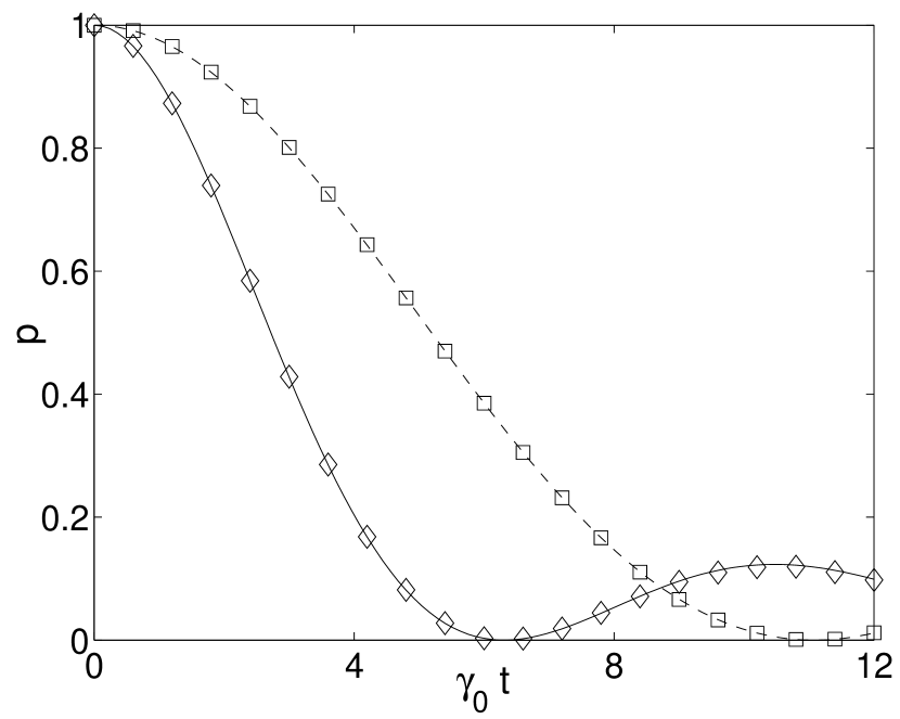
Figure 1: Excited state probability $p(t)$ (Eq. (81)) of the damped Jaynes-Cummings model. Symbols: Monte Carlo simulations of the stochastic differential equations (29) and (30) with ${\mathcal{N}}=5\cdot 10^{6}$ realizations for the parameters $\lambda^{-1}=5\gamma_{0}^{-1}$ (diamonds) and $\lambda^{-1}=20\gamma_{0}^{-1}$ (squares). The corresponding analytical solutions are given by the continuous and the broken line.

The application of the simulation algorithm detailed in Sec. III.1 to this situation is straightforward. In particular, we note that according to Eqs. (70) and (77) the waiting time distribution (40) after an odd number of jumps takes the form

$$F(\tau)=1-\exp\left(-\sqrt{\frac{\gamma_{0}}{2\lambda}}\left[1-e^{-\lambda\tau}\right]\right).$$ (78)

Hence, the probability that no further jumps occur equals

$$q=1-\lim_{\tau\rightarrow\infty}F(\tau)=\exp\left(-\sqrt{\frac{\gamma_{0}}{2\lambda}}\right).$$ (79)

This means that in the case $\eta<q$ no further jumps occur, while in the case $\eta>q$ the random time step is determined by Eq. (71) which yields

$$\tau=-\frac{1}{\lambda}\ln\left(1+\sqrt{\frac{2\lambda}{\gamma_{0}}}\ln\eta\right).$$ (80)

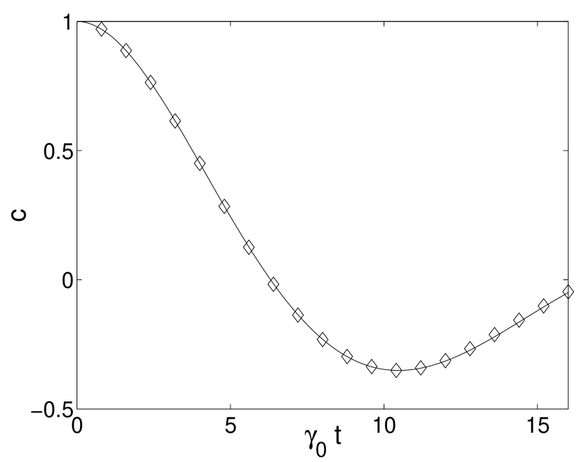
Figure 2: The correlation function $c(t)$ (Eq. (82)) of the damped Jaynes-Cummings model: Analytical solution (continuous line) and Monte Carlo simulation of the stochastic differential equations (29) and (30) (diamonds) for $\lambda^{-1}=5\gamma_{0}^{-1}$ and ${\mathcal{N}}=10^{7}$ realizations.

Results of Monte Carlo simulations of the damped Jaynes-Cummings model are presented in Fig. 1, which shows the population of the excited state,

$$p(t)={\mathrm{E}}\left(\langle e|\psi_{1}\rangle\langle\psi_{2}|e\rangle\langle\chi_{2}|\chi_{1}\rangle\right),$$ (81)

estimated from a sample of realizations of the stochastic process using the estimator described by Eq. (59). As can be seen from the figure, the simulation results reproduce the analytical curves with high accuracy. We note that for the parameter values chosen the reservoir correlation time $\lambda^{-1}$ is larger than the reduced system’s Markovian relaxation time $\gamma_{0}^{-1}$. We therefore observe a pronounced non-Markovian behavior and large deviations form the Born-Markov dynamics. For small and intermediate couplings, the open system dynamics derived from the model described by the interaction Hamiltonian (62) and initial conditions (64) satisfies a time-local master equation of the form $\dot{\rho}_{S}(t)={\mathcal{K}}(t)\rho_{S}(t)$ with a time-dependent super-operator ${\mathcal{K}}(t)$. However, the TCL expansion of the generator ${\mathcal{K}}(t)$ breaks down in the strong coupling regime given by $\lambda^{-1}>\frac{1}{2}\gamma_{0}^{-1}$ for times $t>t_{0}$, where $t_{0}$ denotes the first positive zero of $p(t)$. Beyond the singularity at $t=t_{0}$ the TCL expansion of the master equation is therefore not capable of describing the reduced system dynamics which develops a long memory time of the order $t_{0}$. However, as is exemplified in the figure, the stochastic simulation is seen to describe correctly the full non-Markovian behavior of the reduced system even in the strong coupling regime.

To give an example of the simulation of correlation functions we investigate the quantity $\langle\sigma_{+}(t)\sigma_{-}(0)\rangle$ which can be determined with the help of the method described in Sec. II.3.3. Figure 2 shows the simulation results for the quantity

$$c(t)\equiv e^{-i\omega_{0}t}\langle\sigma_{+}(t)\sigma_{-}(0)\rangle,$$ (82)

which again nicely fit the analytical curve.

III.3 Jaynes-Cummings model with detuning

If the cavity mode is detuned from the atomic transition frequency by an amount $\Delta$ the spectral density becomes

$$J(\omega)=\frac{1}{2\pi}\frac{\gamma_{0}\lambda^{2}}{(\omega_{0}-\Delta-\omega)^{2}+\lambda^{2}},$$ (83)

which leads to the reservoir correlation function

$$f(t^{\prime}-t)=\frac{1}{2}\gamma_{0}\lambda e^{i\Delta(t^{\prime}-t)-\lambda|t^{\prime}-t|}.$$ (84)

We can again use the simulation algorithm described in Sec. III.1, although, by contrast to the previous case, the correlation function (84) is complex-valued. Since the transition rates and the deterministic drift of the process depend on the absolute value of $f$, the only modification of the algorithm for the resonant case appears in Eq. (75) which describes the even jumps into the vacuum state.

An example of the simulation results is shown in Fig. 3. The detuning $\Delta$ influences both the coherent dynamics of the system as well as the dissipation mechanism. This leads to a slower decay and to an oscillatory behavior of the excited state probability, which is correctly reproduced by the stochastic simulation.

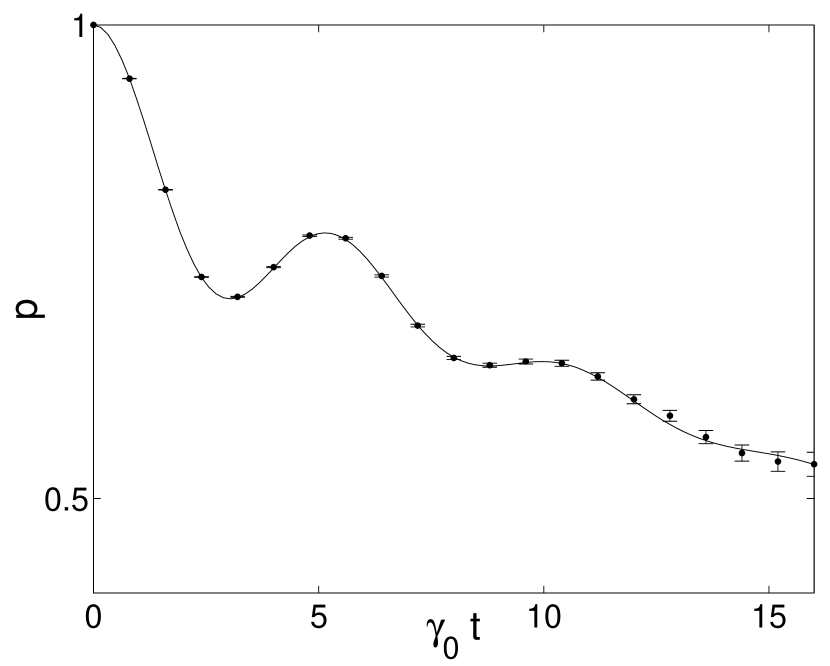
Figure 3: The excited state probability $p(t)$ (Eq. (81)) of the damped Jaynes-Cummings model with detuning: Analytical solution (continuous line) and Monte Carlo simulation of the stochastic differential equations (29) and (30) (dots and errorbars) for $\lambda^{-1}=5\gamma_{0}^{-1}$, $\Delta=\gamma_{0}$ and ${\mathcal{N}}=10^{7}$ realizations.

IV Interaction with a spin bath

The stochastic method developed in Sec. II is not restricted to the treatment of bosonic reservoirs. It is also applicable to the dynamics of open systems coupled to spin environments. As an example, we examine here a specific central spin model which may be used to model the interaction of a single electron spin confined to a quantum dot with a bath of nuclear spins LOSS .

IV.1 Description of the model

The model is defined by the total Hamiltonian

$$H=\frac{\omega_{0}}{2}\sigma_{3}+\sum_{j=1}^{N}A^{(j)}\vec{\sigma}\cdot\vec{\sigma}^{(j)}.$$ (85)

The central spin is represented by the Pauli spin operator $\vec{\sigma}$, while the $N$ bath spins are given by the spin operators $\vec{\sigma}^{(j)}$ with $j=1,2,\ldots,N$. The coupling of the central spin to the $j$th bath spin is described by the constant $A^{(j)}$. For simplicity, the coupling constants are taken to be $A^{(j)}=A/\sqrt{N}$. The corresponding interaction picture Hamiltonian can be written as

$$H_{I}(t)=\sigma_{3}B_{3}(t)+\sigma_{+}B_{-}(t)+\sigma_{-}B_{+}(t)$$ (86)

with

$$B_{3} = \sum_{j}A^{(j)}\sigma_{3}^{(j)},$$ (87)

$$B_{\pm} = \sum_{j}2A^{(j)}\sigma_{\pm}^{(j)}e^{\mp i\omega_{0}t}.$$ (88)

Our aim is to determine the coherence of the central spin,

$$\rho_{+-}(t)=\langle+|\rho_{S}(t)|-\rangle,$$ (89)

where $|\pm\rangle$ are the eigenstates of the 3-component $\sigma_{3}$ of the central spin $\vec{\sigma}$ with eigenvalues $\pm 1$. Within the stochastic simulation technique this quantity is represented through the expectation value (see Eq. (1))

$$\rho_{+-}(t)={\mathrm{E}}\left(\langle+|\psi_{+}\rangle\langle\psi_{-}|-\rangle\langle\chi_{-}|\chi_{+}\rangle\right),$$ (90)

where we write here $|\Phi_{\nu}\rangle\equiv|\Phi_{\pm}\rangle=\psi_{\pm}\otimes\chi_{\pm}$ for the stochastic states, that is the index $\nu$ takes on the values $\nu=\pm$. The initial state is taken to be

$$\rho(0)=|+\rangle\langle-|\otimes\frac{1}{2^{N}}I_{E}.$$ (91)

$I_{E}$ denotes the unit matrix in the $2^{N}$-dimensional state space ${\mathcal{H}}_{E}$ of the spin bath. The spin bath is thus in an unpolarized initial state.

IV.2 Simulation algorithm and results

To apply the simulation technique it is useful to realize the unpolarized initial state $2^{-N}I_{E}$ of the spin bath with the help of an appropriate set of basis states of the Hilbert space ${\cal{H}}_{E}$ spanned by the $N$ bath spins. To this end, we introduce states $|j,m\rangle$ which are defined as simultaneous eigenstates of the square $\vec{J}\,^{2}$ of the total spin angular momentum $\vec{J}$ of the bath and of its 3-component $J_{3}$. The initial state can then be represented by

$$|\Phi_{\pm}(0)\rangle=|\pm\rangle\otimes|j,m\rangle$$ (92)

with an appropriate probability distribution of the corresponding quantum numbers $j$ and $m$ which will be constructed below.

The state $|\Phi_{\pm}(0)\rangle$ defined in (92) is an eigenstate of the 3-component $\frac{1}{2}\sigma_{3}+J_{3}$ of the total spin angular momentum, which is a conserved quantity, corresponding to the eigenvalue $\frac{1}{2}(\pm 1+2m)$. This fact enables us to carry out the canonical transformation $|\Phi_{\pm}(t)\rangle\longrightarrow|\tilde{\Phi}_{\pm}(t)\rangle$ defined by

$$|\Phi_{\pm}(t)\rangle=\exp\left[\frac{-iAt}{\sqrt{N}}\left((\pm 1+2m)\sigma_{3}-1\right)\right]|\tilde{\Phi}_{\pm}(t)\rangle,$$ (93)

which transforms the interaction Hamiltonian (86) into

$$\tilde{H}_{I}(t)=\sigma_{+}B_{-}(t)+\sigma_{-}B_{+}(t).$$ (94)

In this equation the $B_{\pm}(t)$ are given again by Eq. (88), where, however, $\omega_{0}$ must be replaced by the new frequencies $\omega_{\pm}$:

$$\omega_{0}\longrightarrow\omega_{\pm}=\omega_{0}+\frac{2A}{\sqrt{N}}(\pm 1+2m).$$ (95)

In terms of the stochastic states $|\tilde{\Phi}_{\pm}\rangle=\tilde{\psi}_{\pm}\otimes\tilde{\chi}_{\pm}$ the coherence of the central spin is then given by the expectation value

$$\rho_{+-}(t)={\mathrm{E}}\left(e^{-4iAmt/\sqrt{N}}\langle+|\tilde{\psi}_{+}\rangle\langle\tilde{\psi}_{-}|-\rangle\langle\tilde{\chi}_{-}|\tilde{\chi}_{+}\rangle\right).$$ (96)

Summarizing, we can simulate, employing the method developed in Sec. II, the stochastic dynamics corresponding to the new interaction Hamiltonian (94) and estimate the coherence by means of the formula (96). The canonical transformation (93) is accounted for in this formula by the exponential factor $\exp[-4iAmt/\sqrt{N}]$.

In order to see more explicitly how the method works it may be instructive at this point to consider first the simpler model obtained by omitting the terms $\sigma_{\pm}B_{\mp}(t)$ of the interaction Hamiltonian (86). The transformed Hamiltonian (94) is then identically zero and the expression (96) for the coherence of the central spin becomes

$$\rho_{+-}(t)={\mathrm{E}}\left(e^{-4iAmt/\sqrt{N}}\right)=\sum_{m=-N/2}^{+N/2}p_{m}e^{-4iAmt/\sqrt{N}},$$ (97)

where $p_{m}$ is the probability of finding a basis state with quantum number $m$ in the unpolarized initial mixture. Since all basis states are equally likely in this initial mixture, $p_{m}$ is found to be

$$p_{m}=\frac{1}{2^{N}}\binom{N}{\frac{N}{2}+m}.$$ (98)

Here, $2^{N}$ is the total number of basis states of the bath of $N$ spins (the dimension of ${\mathcal{H}}_{E}$), while the binomial coefficient counts the number of basis states corresponding to a given value of $m$. The summation in Eq. (97) can easily be carried out to give

$$\rho_{+-}(t)=\left[\cos\left(\frac{2At}{\sqrt{N}}\right)\right]^{N},$$ (99)

which is the exact expression for the coherence of the central spin. We note that this expression may be approximated by

$$\rho_{+-}(t)=e^{-2A^{2}t^{2}}$$ (100)

in the limit of a large number of bath spins, $N\longrightarrow\infty$, showing an exponential decay of the coherence of the central spin. Thus we see that the stochastic simulation for this simplified model reduces to the generation of a binomially distributed random number $m$ and to the estimation of the expectation value (97).

We turn again to the discussion of the full model described by the Hamiltonian (86). Employing the method described above and using the transformed interaction Hamiltonian (94) we see that the simulation algorithm is quite similar to the one used already in the bosonic case. In fact, the simulation technique turns out to be even simpler. Suppose we have drawn the initial state $|\pm\rangle\otimes|j,m\rangle$. The bath state $\tilde{\chi}_{\pm}(t)$ then jumps between states which are proportional to $|j,m\rangle$ and $|j,m\pm 1\rangle$. The corresponding jump rate

$$\Gamma_{\pm}=2A\sqrt{\frac{j(j+1)-m(m\pm 1)}{N}}$$ (101)

is independent of time. The waiting time of the PDP is therefore always exponentially distributed, which makes the numerical implementation particularly easy for this case. A detailed analysis of the process reveals that the coherence can be represented through the expectation value

$$\rho_{+-}(t) = {\mathrm{E}}\big{(}e^{-4iAmt/\sqrt{N}}(-1)^{(k_{+}+k_{-})/2}e^{(\Gamma_{+}+\Gamma_{-})t}$$ (102)

$$\;\;\;\times\exp(i\omega_{+}(\tau_{2}^{+}+\tau_{4}^{+}\ldots+\tau_{k_{+}}^{+}))$$

$$\;\;\;\times\exp(i\omega_{-}(\tau_{2}^{-}+\tau_{4}^{-}\ldots+\tau_{k_{-}}^{-}))\big{)}.$$

Here, $\tau_{2n}^{\pm}$ denotes the random time step before the $2n$th jump of $|\tilde{\Phi}_{\pm}\rangle$, while $\Gamma_{\pm}$ and $\omega_{\pm}$ have already been defined in Eqs. (101) and (95). The quantity $k_{\pm}$ is defined as the total number of jumps of $|\tilde{\Phi}_{\pm}(t)\rangle$ during the time interval from $0$ to $t$. The integers $k_{\pm}$ may be supposed to be even since only trajectories with an even number of jumps contribute to the expectation value (102).

It remains to explain how to generate, in the general case, the initial states $|j,m\rangle$ in Eq. (92). More precisely, these states should be written as $|\lambda,j,m\rangle$, where $\lambda$ stands for an additional quantum number which, together with $j$ and $m$, uniquely fixes the basis state. The quantum number $\lambda$ corresponds to further observables of the spin bath which commute with $\vec{J}\,^{2}$ and $J_{3}$. If $N$ is even $j$ takes on the values $j=0,1,2,\ldots,\frac{N}{2}$, while $j=\frac{1}{2},\frac{3}{2},\ldots,\frac{N}{2}$ if $N$ is odd. For a given value of $j$ the quantum number $m$ takes on the values $m=-j,-j+1,\ldots,+j$.

In order to achieve that the initial ensemble represents the unpolarized bath state, that is

$${\mathrm{E}}(|\lambda,j,m\rangle\langle\lambda,j,m|)=\frac{1}{2^{N}}I_{E},$$ (103)

all basis states $|\lambda,j,m\rangle$ must occur with the same probability of $2^{-N}$. Since the value of the quantum number $\lambda$ is irrelevant in the simulation scheme, we need the probability $P(j,m)$ of finding the pair of quantum numbers $(j,m)$ in the initial ensemble. This probability can be written as

$$P(j,m)=2^{-N}a_{j}^{N}.$$ (104)

The quantity $a_{j}^{N}$ denotes the number of times a given angular momentum $j$ appears in the decomposition of the Hilbert space ${\mathcal{H}}_{E}$ of $N$ spins into irreducible subspaces of the rotation group. Since a certain $j$-manifold consists of $(2j+1)$ states, distinguished by their values of the quantum number $m$, we can also say that $(2j+1)a_{j}^{N}$ is equal to the number of independent ways the $N$ bath spins can be coupled to give the total angular momentum $j$. For example, the Hilbert space of $N=4$ spins decomposes into two ($j=0$)-manifolds, three ($j=1$)-manifolds, and one ($j=2$)-manifold, that is we have $a_{0}^{4}=2$, $a_{1}^{4}=3$, and $a_{2}^{4}=1$. It may be shown BOSE that $a_{j}^{N}$ is given by the general expression

$$a_{j}^{N}=\binom{N}{\frac{N}{2}+j}-\binom{N}{\frac{N}{2}+j+1}.$$ (105)

We note that $P(j,m)$ is normalized,

$$\sum_{j}\sum_{m=-j}^{+j}P(j,m)=1,$$ (106)

and does of course not depend on $m$. In summary, the quantum numbers $(j,m)$ of the initial ensemble follow the distribution $P(j,m)$ given by the expressions (104) and (105). In the stochastic simulation algorithm one therefore has to generate a sample of random numbers $(j,m)$ with this distribution, which is easily done making use of the inversion method, for example.

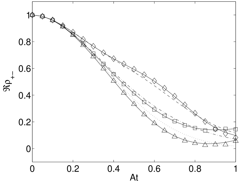
Figure 4: Real part of the coherence (89) of the central spin interacting with a spin bath through the Hamiltonian (86) with $N=10^{3}$. Symbols: Monte Carlo simulation of the stochastic differential equations (29) and (30) using ${\mathcal{N}}=2\cdot 10^{7}$ realizations for the parameters $A/\omega_{0}=0.1$ (diamonds), $A/\omega_{0}=0.2$ (squares), and $A/\omega_{0}=10$ (triangles). Continuous lines: Corresponding solutions of the von Neumann equation (3). The dashed line ($A/\omega_{0}=0.1$), the dashed-dotted line ($A/\omega_{0}=0.2$), and the dotted line ($A/\omega_{0}=10$) show the results obtained from the TCL master equation in second order (Eqs. (108) and (109)).

Examples of Monte Carlo simulations of the central spin model are shown in Fig. 4. One observes that the PDP reproduces the von Neumann dynamics with high accuracy. We do not show errorbars in the figure because the statistical errors are smaller than the size of the symbols. The figure also displays the results found with the help of the second-order TCL master equation of the central spin which is given by

$$\frac{d}{dt}\rho_{S} = -2iA^{2}\frac{1-\cos\omega_{0}t}{\omega_{0}}[\sigma_{3},\rho_{S}]$$

$$-A^{2}t[\sigma_{3},[\sigma_{3},\rho_{S}]]$$

$$+4A^{2}\frac{\sin\omega_{0}t}{\omega_{0}}\left(\sigma_{-}\rho_{S}\sigma_{+}-\frac{1}{2}\{\sigma_{+}\sigma_{-},\rho_{S}\}\right.$$

$$\qquad\qquad\qquad\left.+\sigma_{+}\rho_{S}\sigma_{-}-\frac{1}{2}\{\sigma_{-}\sigma_{+},\rho_{S}\}\right).$$

The solution of this master equation is easily constructed. It yields the expression

$$\rho_{+-}(t)=\exp[-\Gamma(t)]\rho_{+-}(0)$$ (108)

for the coherence of the central spin, where

$$\Gamma(t) = \frac{4iA^{2}t}{\omega_{0}}\left(1-\frac{\sin\omega_{0}t}{\omega_{0}t}\right)$$ (109)

$$+2A^{2}t^{2}\left(1+2\frac{1-\cos\omega_{0}t}{(\omega_{0}t)^{2}}\right).$$

For the parameter values chosen the exact dynamics of the central spin is seen to deviate significantly from the one predicted by the second-order TCL master equation.

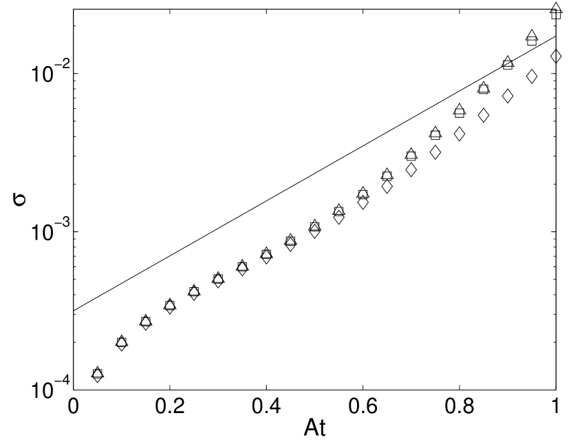
Figure 5: Statistical errors $\sigma(t)$ of Monte Carlo simulations of the central spin model with $10^{7}$ realizations, $A/\omega_{0}=0.5$ and three different values of the number of bath spins: $N=10$ (diamonds), $N=100$ (squares), and $N=1000$ (triangles). The continuous line shows the estimate given by Eq. (111).

Figure 5 presents an example of the behavior of the fluctuations of the stochastic process. The figure shows a plot of the statistical errors $\sigma(t)$ of three Monte Carlo simulations with a fixed number ${\mathcal{N}}$ of realizations, but with three different values of the number $N$ of bath spins. We conclude from the figure that, within the range of time investigated, $\sigma(t)$ is roughly independent of $N$. To understand this behavior we refer to expression (102) which yields

$$\sigma(t)\leq\sqrt{\frac{{\mathrm{E}}\left(\exp[2(\Gamma_{+}+\Gamma_{-})]\right)}{{\mathcal{N}}}}.$$ (110)

The right-hand side of this inequality may be estimated by replacing the random quantities $\Gamma_{\pm}$ by suitable averages using the distribution (104). This gives the estimate

$$\sigma(t)\sim\frac{\exp[4At]}{\sqrt{\mathcal{N}}}.$$ (111)

This expression is indeed independent of $N$ and provides a good estimate of the standard error in the given time interval, as can be seen from the figure. Moreover, this result implies that the fluctuations grow with a rate which is much smaller than the one provided by the strict upper bound $2\Gamma_{0}$ of $\Gamma_{+}+\Gamma_{-}$. In fact, $\Gamma_{0}$ scales with the square root of $N$ which predicts a much stronger increase of the fluctuations.

V Conclusions

It has been shown in this paper that the von Neumann dynamics of a combined quantum system can be formulated in terms of a rather simple piecewise deterministic process which gives rise to a powerful and efficient Monte Carlo simulation method of the exact non-Markovian reduced system behavior. A Markovian representation of the dynamics was achieved through the use of a pair of product states $\psi_{\nu}\otimes\chi_{\nu}$ in the state space of the total system. The stochastic propagation of an ensemble of such pairs then enables one to mimic the exact time-evolution of the reduced system’s density matrix.

The examples discussed in Sec. III and IV illustrate the generality of the method: It is applicable to both bosonic and spin environments and is not restricted to linear dissipation or to a perturbation treatment of the system-environment coupling. Most importantly, the method does not require the derivation, not even the existence of a master equation of the reduced system. At the same time, the technique allows the direct determination of all kinds of multitime quantum correlation functions. Although our discussion was carried out in the interaction picture, it is obvious that the stochastic dynamics can also be formulated in the Schrödinger picture, in which case both $\psi_{\nu}$ and $\chi_{\nu}$ follow, in general, a non-trivial deterministic evolution. Furthermore, it should be clear that, instead of using a PDP, one can also employ a diffusion process (Brownian motion) to construct an unraveling of the von Neumann equation.

The stochastic technique was formulated here as a method of simulating the dynamics of open systems in real time. A potential extension of the method is to re-formulate the dynamics in imaginary time CARUSO2 , in order to determine the properties of the system in thermodynamic equilibrium. With the total Hamiltonian $H=H_{S}+H_{E}+H_{I}$ in the Schrödinger picture the canonical equilibrium density matrix (not normalized) is given by $\rho(\beta)=e^{-\beta H}$, where $\beta=1/k_{\mathrm{B}}T$ is the inverse temperature. At infinite temperature we have $\rho(\beta=0)=I$. This suggests determining the equilibrium density at finite temperature by solving the evolution equation

$$\frac{d}{ds}\rho(s)=-\frac{1}{2}\left\{H,\rho(s)\right\}$$ (112)

over the interval from $s=0$ to $s=\beta$. This imaginary-time dynamics can again be represented in terms of a stochastic process for a pair of product states $|\Phi_{\nu}(s)\rangle=\psi_{\nu}(s)\otimes\chi_{\nu}(s)$. An appropriate system of stochastic differential equations in the Schrödinger picture is given by

$$d\psi_{\nu} = -\frac{1}{2}H_{S}\psi_{\nu}ds$$ (113)

$$+\sum_{\alpha}\left(-\frac{1}{2}L_{\alpha\nu}A_{\alpha}-I\right)\psi_{\nu}dN_{\alpha\nu},$$

$$d\chi_{\nu} = \left(-\frac{1}{2}H_{B}+\Gamma_{\nu}\right)\chi_{\nu}ds$$ (114)

$$+\sum_{\alpha}\left(M_{\alpha\nu}B_{\alpha}-I\right)\chi_{\nu}dN_{\alpha\nu}.$$

Performing a calculation analogous to the one of Sec. II.1 it is easy to verify that the expectation value $\rho(s)={\mathrm{E}}(|\Phi_{1}(s)\rangle\langle\Phi_{2}(s)|)$ satisfies the evolution equation (112). The $dN_{\alpha\nu}(s)$ are again independent Poisson increments satisfying ${\mathrm{E}}(dN_{\alpha\nu}(s))=\Gamma_{\alpha\nu}ds$, and the relations (22) and (23) remain valid.

An important restriction of the Monte Carlo technique is provided by the behavior of the statistical fluctuations. The considerations of Sec. II.2 as well as the example discussed in Sec. IV.2 reveal that the method as formulated in Sec. II.1 is feasible, in general, only for short and intermediate time scales. For large times statistical errors may grow exponentially fast, ruling out the estimation of statistical quantities with reasonable effort. However, this conclusion rests on the assumption that the stochastic states $|\Phi_{\nu}(t)\rangle$ are tensor products of certain system and environment states. This leads to a further potential generalization of the method, namely to introduce a class of stochastic states with a more complicated structure, the aim being a more efficient representation of $\rho(t)$ as the expectation value over the corresponding random process.

Since the interaction generally creates correlations between the states of system and environment it could be advantageous, e. g., to use a class of entangled stochastic states. The spin bath model studied in Sec. IV leads to a trivial example: The class of entangled states defined by ($\alpha$ and $\beta$ are complex amplitudes)

$$\alpha|+\rangle\otimes|j,m\rangle+\beta|-\rangle\otimes|j,m+1\rangle$$ (115)

yields an extremely efficient stochastic representation of the dynamics: As a consequence of the conservation of the 3-component of the total spin angular momentum, the subspaces spanned by the states $|+\rangle\otimes|j,m\rangle$ and $|-\rangle\otimes|j,m+1\rangle$ are invariant under the time-evolution and, thus, the dynamics may be expressed entirely though an appropriate (deterministic) time-dependence of the amplitudes $\alpha$ and $\beta$. Therefore, only the initial state is a random quantity and the statistical errors are constant in time.

In a further possible extension of the method one could employ a stochastic evolution of mixed states instead of pure states. As an example we introduce a stochastic matrix

$$R(t)=|\psi_{1}(t)\rangle\langle\psi_{2}(t)|\otimes R_{E}(t),$$ (116)

where the $\psi_{\nu}(t)$ are random states of the open system and $R_{E}(t)$ is a random operator in ${\mathcal{H}}_{E}$, and try again to find stochastic evolution equations such that the exact von Neumann dynamics is recovered by means of the expectation value $\rho(t)={\mathrm{E}}(R(t))$. This is indeed possible if we use the stochastic differential equations (29) for the $\psi_{\nu}(t)$ and if we replace (30) by the following stochastic differential equation for the random operator $R_{E}(t)$,

$$dR_{E} = \Gamma R_{E}dt+\sum_{\alpha}\left(M_{\alpha 1}B_{\alpha}-I\right)R_{E}dN_{\alpha 1}$$ (117)

$$+\sum_{\alpha}R_{E}\left(M_{\alpha 2}B^{\dagger}_{\alpha}-I\right)dN_{\alpha 2},$$

where $\Gamma=\Gamma_{1}+\Gamma_{2}=\sum_{\alpha\nu}\Gamma_{\alpha\nu}$ is the total jump rate. The further development of the stochastic technique proposed in this paper should include a systematic investigation of the potentialities of the extensions indicated above.

- (1) C. Cohen-Tannoudji, J. Dupont-Roc, and G. Grynberg, Atom-Photon Interactions (John Wiley, New York, 1998).
- (2) C. W. Gardiner and P. Zoller, Quantum Noise (Springer-Verlag, Berlin, 2000).
- (3) S. Nakajima, Progr. Theor. Phys. 20, 948 (1958).
- (4) R. Zwanzig, J. Chem. Phys. 33, 1338 (1960).
- (5) R. P. Feynman and F. L. Vernon, Ann. Phys. (N.Y.) 24, 118 (1963).
- (6) A. O. Caldeira and A. J. Leggett, Physica 121A, 587 (1983).
- (7) H. P. Breuer and F. Petruccione, The Theory of Open Quantum Systems (Oxford University Press, Oxford, 2002).
- (8) G. M. Moy, J. J. Hope, and C. M. Savage, Phys. Rev. A 59, 667 (1999); Phys. Rev. A 61, 023603 (2000).
- (9) G. M. Palma, K.-A. Suominen, A. K. Ekert, Proc. R. Soc. Lond. A 452, 567 (1996).
- (10) N. V. Prokof’ev and P. C. E. Stamp, Rep. Prog. Phys. 63, 669 (2000).
- (11) J. Dalibard, Y. Castin, and K. Mølmer, Phys. Rev. Lett. 68, 580 (1992); R. Dum, P. Zoller, and H. Ritsch, Phys. Rev. A 45, 4879 (1992); N. Gisin and I. C. Percival, J. Math. Phys. A: Math. Gen. 25, 5677 (1992); H. Carmichael, An Open Systems Approach to Quantum Optics, Lecture Notes in Physics m18 (Springer-Verlag, Berlin, 1993); M. B. Plenio and P. L. Knight, Rev. Mod. Phys. 70, 101 (1998); A. Imamoglu and Y. Yamamoto, Phys. Lett. A 191, 425 (1994); A. Imamoglu, Phys. Rev. A 50, 3650 (1994).
- (12) L. Diosi, N. Gisin, and W. T. Strunz, Phys. Rev. A 58, 1699 (1998); W. T. Strunz, L. Diosi, and N. Gisin, Phys. Rev. Lett. 82, 1801 (1999).
- (13) H. P. Breuer, B. Kappler, and F. Petruccione, Phys. Rev. A 59, 1633 (1999).
- (14) J. T. Stockburger and H. Grabert, Phys. Rev. Lett. 88, 170407 (2002).
- (15) H. P. Breuer, quant-ph/0308052.
- (16) I. Carusotto, Y. Castin, and J. Dalibard, Phys. Rev. A 63, 023606 (2001).
- (17) O. Juillet and Ph. Chomaz, Phys. Rev. Lett. 88, 142503 (2002).
- (18) H. P. Breuer, B. Kappler, and F. Petruccione, Phys. Rev. A 56, 2334 (1997).
- (19) A. V. Khaetskii, D. Loss, and L. Glazman, Phys. Rev. Lett. 88, 186802 (2002).
- (20) A. Hutton and S. Bose, quant-ph/0208114.
- (21) I. Carusotto and Y. Castin, J. Phys. B: At. Mol. Opt. Phys. 34, 4589 (2001).