Robust quantum parameter estimation: coherent magnetometry with feedback

Abstract

We describe the formalism for optimally estimating and controlling both the state of a spin ensemble and a scalar magnetic field with information obtained from a continuous quantum limited measurement of the spin precession due to the field. The full quantum parameter estimation model is reduced to a simplified equivalent representation to which classical estimation and control theory is applied. We consider both the tracking of static and fluctuating fields in the transient and steady state regimes. By using feedback control, the field estimation can be made robust to uncertainty about the total spin number.

I Introduction

As experimental methods for manipulating physical systems near their fundamental quantum limits improve Armen et al. (2002); Geremia et al. (2003a); Smith et al. (2002); Morrow et al. (2002); Fischer et al. (2002), the need for quantum state and parameter estimation methods becomes critical. Integrating a modern perspective on quantum measurement theory with the extensive methodologies of classical estimation and control theory provides new insight into how the limits imposed by quantum mechanics affect our ability to measure and control physical systems Verstraete et al. (2001); Gambetta and Wiseman (2001); Mabuchi (1996); Belavkin (1999).

In this paper, we illustrate the processes of state estimation and control for a continuously-observed, coherent spin ensemble (such as an optically pumped cloud of atoms) interacting with an external magnetic field. In the situation where the magnetic field is either zero or well-characterized, continuous measurement (e.g., via the dispersive phase shift or Faraday rotation of a far off-resonant probe beam) can produce a spin-squeezed Kitagawa and Ueda (1993) state conditioned on the measurement record Kuzmich et al. (2000). Spin-squeezing indicates internal entanglement between the different particles in the ensemble Stockton et al. (2003) and promises to improve precision measurements Wineland et al. (1994). When, however, the ambient magnetic environment is either unknown or changing in time, the external field can be estimated by observing Larmor precession in the measurement signal Geremia et al. (2003a); Smith et al. (2003); Kominis et al. (2003); Budker et al. (2002), see Figure 1. Recently, we have shown that uncertainty in both the magnetic field and the spin ensemble can be simultaneously reduced through continuous measurement and adequate quantum filtering Geremia et al. (2003b).

Here, we expand on our recent results Geremia et al. (2003b) involving Heisenberg-limited magnetometry by demonstrating the advantages of including feedback control in the estimation process. Feedback is a ubiquitous concept in classical applications because it enables precision performance despite the presence of potentially large system uncertainty. Quantum optical experiments are evolving to the point where feedback can been used, for example, to stabilize atomic motion within optical lattices Morrow et al. (2002) and high finesse cavities Fischer et al. (2002). Recently, we demonstrated the use of feedback on a polarized ensemble of laser-cooled Cesium atoms to robustly estimate an applied magnetic field Geremia et al. (2003a). In this work, we investigate the theoretical limits of such an approach and demonstrate that an external magnetic field can be measured with high precision despite substantial ignorance of the size of the spin ensemble.

The paper is organized as follows. In Section II, we provide a general introduction to quantum parameter estimation followed by a specialization to the case of a continuously measured spin ensemble in a magnetic field. By capitalizing on the Gaussian properties of both coherent and spin-squeezed states, we formulate the parameter estimation problem in such a way that techniques from classical estimation theory apply to the quantum system. Section III presents basic filtering and control theory in a pedagogical manner with the simplified spin model as an example. This theory is applied in Section IV, where we simultaneously derive mutually dependent magnetometry and spin-squeezing limits in the ideal case where the observer is certain of the spin number. We consider the optimal measurement of both constant and fluctuating fields in the transient and steady state regimes. Finally, we show in Section V that the estimation can be made robust to uncertainty about the total spin number by using precision feedback control.

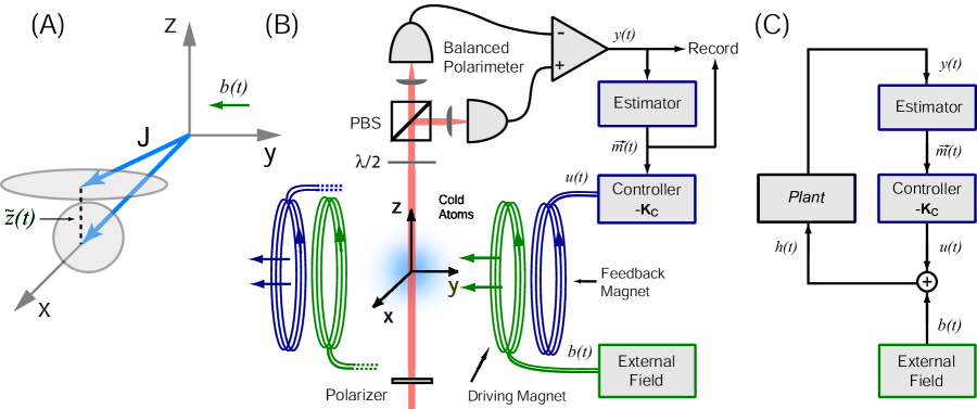
Figure 1: (A) A spin ensemble is initially prepared in a coherent state polarized along x, with symmetric variance in the y and z directions. Subsequently, a field along y causes the spin to rotate as the z-component is continuously measured. (B) Experimental schematic for the measurement process. A far off resonant probe beam traverses the sample and measures the z-component of spin via Faraday rotation. The measurement strength could be improved by surrounding the ensemble with a cavity. (C) Experimental apparatus subsumed by the Plant block, which serves to map the total field to the photocurrent, $h(t)\rightarrow y(t)$.

II Quantum parameter estimation

First, we present a generic description of quantum parameter estimation Verstraete et al. (2001); Gambetta and Wiseman (2001); Mabuchi (1996); Belavkin (1999). This involves describing the quantum system with a density matrix and our knowledge of the unknown parameter with a classical probability distribution. The objective of parameter estimation is then to utilize information gained about the system through measurement to conditionally update both the density matrix and the parameter distribution. After framing the general case, our particular example of a continuously measured spin ensemble is introduced.

II.1 General problem

The following outline of the parameter estimation process could be generalized to treat a wide class of problems (discrete measurement, multiple parameters), but for simplicity, we will consider a continuously measured quantum system with scalar Hamiltonian parameter $\theta$ and measurement record $y(t)$.

Suppose first that the observer has full knowledge of the parameter $\theta$. The proper description of the system would then be a density matrix $\rho_{\theta}(t)$ conditioned on the measurement record $y(t)$. The first problem is to find a rule to update this density matrix with the knowledge obtained from the measurement. As in the problem of this paper, this mapping may take the form of a stochastic master equation (SME). The SME is by definition a filter that maps the measurement record to an optimal estimate of the system state.

Now if we allow for uncertainty in $\theta$, then a particularly intuitive choice for our new description of the system is

$$\rho(t) \equiv \int_{\theta}\rho_{\theta}(t)p(\theta,t)\,d\theta$$ (1)

where $p(\theta,t)$ is a probability distribution representing our knowledge of the system parameter. In addition to the rule for updating each $\rho_{\theta}(t)$, we also need to find a rule for updating $p(\theta,t)$ according to the measurement record. By requiring internal consistency, it is possible to find a Bayes rule for updating $p(\theta,t)$ Verstraete et al. (2001). These two update rules in principle solve the estimation problem completely.

Because evolving $\rho(t)$ involves performing calculations with the full Hilbert space in question, which is often computationally expensive, it is desirable to find a reduced description of the system. Fortunately, it is often possible to find a closed set of dynamical equations for a small set of moments of $\rho(t)$. For example, if $c$ is an observable, then we can define the estimate moments

$$\langle c\rangle(t) \equiv \textrm{Tr}[\rho(t)c]$$

$$\langle\Delta c^{2}\rangle(t) \equiv \textrm{Tr}[\rho(t)(c-\langle c\rangle)^{2}]$$

$$\langle\theta\rangle(t) \equiv \int p(\theta,t)\theta d\theta$$

$$\langle\Delta\theta^{2}\rangle(t) \equiv \int p(\theta,t)(\theta-\langle\theta\rangle)^{2}d\theta$$

and derive their update rules from the full update rules, resulting in a set of $y(t)$-dependent differential equations. If those differential equations are closed, then this reduced description is adequate for the parameter estimation task at hand. This situation (with closure and Gaussian distributions) is to be expected when the system is approximately linear.

II.2 Continuously measured spin system

This approach can be applied directly to the problem of magnetometry considered in this paper. The problem can be summarized by the situation illustrated in Figure 1: a spin ensemble of possibly unknown number is initially polarized along the x-axis (e.g., via optical pumping), an unknown possibly fluctuating scalar magnetic field $b$ directed along the y-axis causes the spins to then rotate within the x-z plane, and the z-component of the collective spin is measured continuously. The measurement can, for example, be implemented as shown, where we observe the difference photocurrent, $y(t)$, in a polarimeter which measures the Faraday rotation of a linearly polarized far off resonant probe beam travelling along z Geremia et al. (2003a); Smith et al. (2003); Silberfarb and Deutsch (2003). The goal is to optimally estimate $b(t)$ via the measurement record and unbiased prior information. If a control field $u(t)$ is included, as it will be eventually, the total field is represented by $h(t)=b(t)+u(t)$.

In terms of our previous discussion, we have here the observable $c=\sqrt{M}J_{z}$, where $M$ is the measurement rate (defined in terms of probe beam parameters), and the parameter $\theta=b$. When $b$ is known, our state estimate evolves by the stochastic master equation Thomsen et al. (2002)

$$d\rho_{b}(t)=-i[H(b),\rho_{b}(t)]dt+\mathcal{D}[\sqrt{M}J_{z}]\rho_{b}(t)dt$$

$$+\sqrt{\eta}\mathcal{H}[\sqrt{M}J_{z}]\left(2\sqrt{M\eta}[y(t)dt-\langle J_{z}\rangle_{b}dt]\right)\rho_{b}(t)$$ (2)

where $H(b)=\gamma J_{y}b$, $\gamma$ is the gyromagnetic ratio, and

$$\mathcal{D}[c]\rho \equiv c\rho c^{\dagger}-(c^{\dagger}c\rho+\rho c^{\dagger}c)/2$$

$$\mathcal{H}[c]\rho \equiv c\rho+\rho c^{\dagger}-\textrm{Tr}[(c+c^{\dagger})\rho]\rho$$

The stochastic quantity $2\sqrt{M\eta}[y(t)dt-\langle J_{z}\rangle_{b}(t)dt]\equiv d\bar{W}(t)$ is a Wiener increment (Gaussian white noise with variance $dt$) by the optimality of the filter. The sensitivity of the photodetection per $\sqrt{\textrm{Hz}}$ is represented by $1/2\sqrt{M\eta}$, where the quantity $\eta$ represents the quantum efficiency of the detection. If $\eta=0$, we are essentially ignoring the measurement result and the conditional SME becomes a deterministic unconditional master equation. If $\eta=1$, the detectors are maximally efficient. Note that our initial state $\rho(0)=\rho_{b}(0)$ is made equal to a coherent state (polarized in x) and is representative of our prior information.

It can be shown that the unnormalized probability $\bar{p}(b,t)$ evolves according to Verstraete et al. (2001)

$$d\bar{p}(b,t)=4M\eta\langle J_{z}\rangle_{b}(t)\bar{p}(b,t)y(t)dt$$ (3)

The evolution Eqs. (2) and (3) together with Eq. (1) solve the problem completely, albeit in a computationally expensive way. Clearly, for large ensembles it would be advantageous to reduce the problem to a simpler description.

If we consider only the estimate moments $\langle J_{z}\rangle(t)$, $\langle\Delta J_{z}^{2}\rangle(t)$, $\langle b\rangle(t)$, and $\langle\Delta b^{2}\rangle(t)$ and derive their evolution with the above rules, it can be shown that the filtering equations for those variables are closed under certain approximations. First, the spin number $J$ must be large enough that the distributions for $J_{y}$ and $J_{z}$ are approximately Gaussian for an x-polarized coherent state. Second, we only consider times $t\ll 1/M$ because the total spin becomes damped by the measurement at times comparable to the inverse of the measurement rate.

Although this approach is rigorous and fail-safe, the resulting filtering equations for the moments can be arrived at in a more direct manner as discussed in Appendix A. Essentially, the full quantum mechanical mapping from $h(t)$ to $y(t)$ is equivalent to the mapping derived from a model which appears classical, and assumes an actual, but random, value for the $z$ component of spin. This correspondence generally holds for a stochastic master equation corresponding to an arbitrary linear quantum mechanical system with continuous measurement of observables that are linear combinations of the canonical variables Doherty and Wiseman (2003).

From this point on we will only consider the simplified Gaussian representation (used in the next section) since it allows us to apply established techniques from estimation and control theory. The replacement of the quantum mechanical model with a classical noise model is discussed more fully in the appendix. Throughout this treatment, we keep in mind the constraints that the original model imposed. As before, we assume $J$ is large enough to maintain the Gaussian approximation and that time is small compared to the measurement induced damping rate, $t\ll 1/M$. Also, the description of our original problem demands that $\langle\Delta J_{z}^{2}\rangle(0)=J/2$ for a coherent state . Hence our prior information for the initial value of the spin component will always be dictated by the structure of Hilbert space.

III Optimal estimation and control

We now describe the dynamics of the simplified representation. Given a linear state-space model (L), a quadratic performance criterion (Q) and Gaussian noise (G), we show how to apply standard LQG analysis to optimize the estimation and control performance Jacobs (1996).

The system state we are trying to estimate is represented by

State

$$\vec{x}(t) \equiv \begin{bmatrix}z(t)\\ b(t)\end{bmatrix}$$ (4)

where $z(t)$ represents the small z-component of the collective angular momentum and $b(t)$ is a scalar field along the y axis.

Our best guess of $\vec{x}(t)$, as we filter the measurement record, will be denoted

Estimate

$$\vec{m}(t) \equiv \begin{bmatrix}\tilde{z}(t)\\ \tilde{b}(t)\end{bmatrix}$$ (5)

As stated in the appendix, we implicitly make the associations: $\tilde{z}(t)=\langle J_{z}\rangle(t)=\textrm{Tr}[\rho(t)J_{z}]$ and $\tilde{b}(t)=\int p(b,t)b\,db$, although no further mention of $\rho(t)$ or $p(b,t)$ will be made.

We assume the measurement induced damping of $J$ to be negligible for short times ($J\exp[-Mt/2]\approx J$ if $t\ll 1/M$) and approximate the dynamics as

Dynamics

$$d\vec{x}(t) = \textbf{A}\vec{x}(t)dt+\textbf{B}u(t)dt+\begin{bmatrix}0\\ \sqrt{\sigma_{bF}}\end{bmatrix}dW_{1}$$ (6)

A $$\equiv \begin{bmatrix}0&\gamma J\\ 0&-\gamma_{b}\end{bmatrix}$$

B $$\equiv \begin{bmatrix}\gamma J\\ 0\end{bmatrix}$$

$$\mathbf{\Sigma_{0}} \equiv \begin{bmatrix}\sigma_{z0}&0\\ 0&\sigma_{b0}\end{bmatrix}$$

$$\mathbf{\Sigma_{1}} \equiv \begin{bmatrix}0&0\\ 0&\sigma_{bF}\end{bmatrix}$$

where the initial value $\vec{x}(0)$ for each trial is drawn randomly from a Gaussian distribution of mean zero and covariance matrix $\mathbf{\Sigma}_{0}$. The initial field variance $\sigma_{b0}$ is considered to be due to classical uncertainty, whereas the initial spin variance $\sigma_{z0}$ is inherently non-zero due to the original quantum state description. Specifically, we impose $\sigma_{z0}=\langle\Delta J_{z}^{2}\rangle(0)$. The Wiener increment $dW_{1}(t)$ has a Gaussian distribution with mean zero and variance $dt$. $\mathbf{\Sigma_{1}}$ represents the covariance matrix of the last vector in Eq. (6).

We have given ourselves a magnetic field control input, $u(t)$, along the same axis, y, of the field to be measured, $b(t)$. We have allowed $b(t)$ to fluctuate via a damped diffusion (Ornstein-Uhlenbeck) process Gardiner (1985)

$$db(t) = -\gamma_{b}b(t)\,dt+\sqrt{\sigma_{bF}}\,dW_{1}$$ (7)

The $b(t)$ fluctuations are represented in this particular way because Gaussian noise processes are amenable to LQG analysis. The variance of the field at any particular time is given by the expectation $\sigma_{bFree}\equiv\textrm{E}[b(t)^{2}]=\sigma_{bF}/2\gamma_{b}$. (Throughout the paper we use the notation $\textrm{E}[x(t)]$ to represent the average of the generally stochastic variable $x(t)$ at the same point in time, over many trajectories.) The bandwidth of the field is determined by the frequency $\gamma_{b}$ alone. When considering the measurement of fluctuating fields, a valid choice of prior might be $\sigma_{b0}=\sigma_{bFree}$, but we choose to let $\sigma_{b0}$ remain independent. For constant fields, we set $\sigma_{bFree}=0$, but $\sigma_{b0}\neq 0$.

Note that only the small angle limit of the spin motion is considered. Otherwise we would have to consider different components of the spin vector rotating into each other. The small angle approximation would be invalid if a field caused the spins to rotate excessively, but using adequate control ensures this will not happen. Hence, we use control for essentially two reasons in this paper: first to keep our small angle approximation valid, and, second, to make our estimation process robust to our ignorance of $J$. The latter point will be discussed in Section V.

Our measurement of $z$ is described by the process

Measurement

$$y(t)dt = \textbf{C}\vec{x}(t)dt+\sqrt{\sigma_{M}}dW_{2}(t)$$ (8)

C $$\equiv \begin{bmatrix}1&0\end{bmatrix}$$

$$\mathbf{\Sigma_{2}} \equiv \sigma_{M}\equiv 1/4M\eta$$

where the measurement shot-noise is represented by the Wiener increment $dW_{2}(t)$ of variance $dt$. Again, $\sqrt{\sigma_{M}}$ represents the sensitivity of the measurement, $M$ is the measurement rate (with unspecified physical definition in terms of probe parameters), and $\eta$ is the quantum efficiency of the measurement. The increments $dW_{1}$ and $dW_{2}$ are uncorrelated.

Following Jacobs (1996), the optimal estimator for mapping $y(t)$ to $\vec{m}(t)$ takes the form

Estimator

$$d\vec{m}(t) = \textbf{A}\vec{m}(t)dt+\textbf{B}u(t)dt$$ (9)

$$+\textbf{K}_{O}(t)[y(t)-\textbf{C}\vec{m}(t)]dt$$

$$\vec{m}(0) = \begin{bmatrix}0\\ 0\end{bmatrix}$$

$$\textbf{K}_{O}(t) \equiv \mathbf{\Sigma}(t)\textbf{C}^{T}\mathbf{\Sigma}_{2}^{-1}$$

$$\frac{d\mathbf{\Sigma}(t)}{dt} = \mathbf{\Sigma}_{1}+\textbf{A}\mathbf{\Sigma}(t)+\mathbf{\Sigma}(t)\textbf{A}^{T}$$ (10)

$$-\mathbf{\Sigma}(t)\textbf{C}^{T}\mathbf{\Sigma}_{2}^{-1}\textbf{C}\mathbf{\Sigma}(t)$$

$$\mathbf{\Sigma}(t) \equiv \begin{bmatrix}\sigma_{zR}(t)&\sigma_{cR}(t)\\ \sigma_{cR}(t)&\sigma_{bR}(t)\end{bmatrix}$$ (11)

$$\mathbf{\Sigma}(0) = \mathbf{\Sigma_{0}}\equiv\begin{bmatrix}\sigma_{z0}&0\\ 0&\sigma_{b0}\end{bmatrix}$$ (12)

Eq. (9) is the Kalman filter which depends on the solution of the matrix Riccati Eq. (10). The Riccati equation gives the optimal observation gain $\textbf{K}_{O}(t)$ for the filter. The estimator is designed to minimize the average quadratic estimation error for each variable: $\textrm{E}[(z(t)-\tilde{z}(t))^{2}]$ and $\textrm{E}[(b(t)-\tilde{b}(t))^{2}]$. If the model is correct, and we assume the observer chooses his prior information $\mathbf{\Sigma}(0)$ to match the actual variance of the initial data $\mathbf{\Sigma_{0}}$, then we have the self-consistent result:

$$\sigma_{zE}(t) \equiv \textrm{E}[(z(t)-\tilde{z}(t))^{2}]=\sigma_{zR}(t)$$

$$\sigma_{bE}(t) \equiv \textrm{E}[(b(t)-\tilde{b}(t))^{2}]=\sigma_{bR}(t)$$

Hence, the Riccati equation solution represents both the observer gain and the expected performance of an optimal filter using that same gain.

Now consider the control problem, which is in many respects dual to the estimation problem. We would like to design a controller to map $y(t)$ to $u(t)$ in a manner that minimizes the quadratic cost function

Minimized Cost

$$H = \int_{0}^{T}\left[\vec{x}^{T}(t)\textbf{P}\vec{x}(t)+u(t)\textbf{Q}u(t)\right]\,dt$$ (13)

$$+\vec{x}^{T}(T)\textbf{P}_{1}\vec{x}(T)$$

$$\mathbf{P} \equiv \begin{bmatrix}p&0\\ 0&0\end{bmatrix}$$

$$\mathbf{Q} \equiv q$$

where $\textbf{P}_{1}$ is the end-point cost. Only the ratio $p/q$ ever appears, of course, so we define the parameter $\lambda\equiv\sqrt{p/q}$ and use it to represent the cost of control. By setting $\lambda\rightarrow\infty$, as we often choose to do in the subsequent analysis to simplify results, we are putting no cost on our control output. This is unrealistic because, for example, making $\lambda$ arbitrarily large implies that we can apply transfer functions with finite gain at arbitrarily high frequencies, which is not experimentally possible. Despite this, we will often consider the limit $\lambda\rightarrow\infty$ to set bounds on achievable estimation and control performance. The optimal controller for minimizing Eq. (13) is

Controller

$$u(t) = -\textbf{K}_{C}(t)\vec{m}(t)$$ (14)

$$\textbf{K}_{C}(t) \equiv \textbf{Q}^{-1}\textbf{B}^{T}\textbf{V}(T-t)$$

$$\frac{d\textbf{V}(T)}{dT} = \textbf{P}+\textbf{A}^{T}\textbf{V}(T)+\textbf{V}(T)\textbf{A}$$ (15)

$$-\textbf{V}(T)\textbf{B}\textbf{Q}^{-1}\textbf{B}^{T}\textbf{V}(T)$$

$$\textbf{V}(T=0) \equiv \textbf{P}_{1}$$

Here $\textbf{V}(T)$ is solved in reverse time $T$, which can be interpreted as the time left to go until the stopping point. Thus if $T\rightarrow\infty$, then we only need to use the steady state of the V Riccati Eq. (15) to give the steady state controller gain $\textbf{K}_{C}$ for all times. In this case, we can ignore the (reverse) initial condition $P_{1}$ because the controller is not designed to stop. Henceforth, we will make $\textbf{K}_{C}$ equal to this constant steady state value, such that the only time varying coefficients will come from $\textbf{K}_{O}(t)$.

In principle, the above results give the entire solution to the ideal estimation and control problem. However, in the non-ideal case where our knowledge of the system is incomplete, e.g. $J$ is unknown, our estimation performance will suffer. Notation is now introduced which produces trivial results in the ideal case, but is helpful otherwise. Our goal is to collect the above equations into a single structure which can be used to solve the non-ideal problem. We define the total state of the system and estimator as

Total State

$$\vec{\theta}(t) \equiv \begin{bmatrix}\vec{x}(t)\\ \vec{m}(t)\end{bmatrix}=\begin{bmatrix}z(t)\\ b(t)\\ \tilde{z}(t)\\ \tilde{b}(t)\end{bmatrix}$$ (16)

Consider the general case where the observer assumes the plant contains spin $J^{\prime}$, which may or may not be equal to the actual $J$. All design elements depending on $J^{\prime}$ instead of $J$ are now labelled with a prime. Then it can be shown that the total state dynamics from the above estimator-controller architecture are a time-dependent Ornstein-Uhlenbeck process

Total State Dynamics

$$d\vec{\theta}(t) = \mathbf{\alpha}(t)\vec{\theta}(t)dt+\mathbf{\beta}(t)d\vec{W}(t)$$ (17)

$$\mathbf{\alpha}(t) \equiv \begin{bmatrix}\textbf{A}&-\textbf{B}\textbf{K}^{\prime}_{C}\\ \textbf{K}^{\prime}_{O}(t)\textbf{C}&\textbf{A}^{\prime}-\textbf{B}^{\prime}\textbf{K}^{\prime}_{C}-\textbf{K}^{\prime}_{O}(t)\textbf{C}\end{bmatrix}$$

$$\mathbf{\beta}(t) \equiv \begin{bmatrix}0&0&0&0\\ 0&\sqrt{\sigma_{bF}}&0&0\\ 0&0&\sqrt{\sigma_{M}}K^{\prime}_{O1}(t)&0\\ 0&0&\sqrt{\sigma_{M}}K^{\prime}_{O2}(t)&0\end{bmatrix}$$

where the covariance matrix of $d\vec{W}$ is $dt$ times the identity. Now the quantity of interest is the following covariance matrix

Total State Covariance

$$\mathbf{\Theta}(t) \equiv \textrm{E}[\vec{\theta}(t)\vec{\theta}^{T}(t)]$$ (18)

$$\equiv \begin{bmatrix}\sigma_{zz}&\sigma_{zb}&\sigma_{z\tilde{z}}&\sigma_{z\tilde{b}}\\ \sigma_{zb}&\sigma_{bb}&\sigma_{b\tilde{z}}&\sigma_{b\tilde{b}}\\ \sigma_{z\tilde{z}}&\sigma_{b\tilde{z}}&\sigma_{\tilde{z}\tilde{z}}&\sigma_{\tilde{z}\tilde{b}}\\ \sigma_{z\tilde{b}}&\sigma_{b\tilde{b}}&\sigma_{\tilde{z}\tilde{b}}&\sigma_{\tilde{b}\tilde{b}}\end{bmatrix}$$

$$\sigma_{zz} \equiv \textrm{E}[z(t)^{2}]$$

$$\sigma_{zb} \equiv \textrm{E}[z(t)b(t)]$$

$$\vdots \equiv \vdots$$

It can be shown that this total covariance matrix obeys the deterministic equations of motion

Total State Covariance Dynamics

$$\frac{d\mathbf{\Theta}(t)}{dt} = \mathbf{\alpha}(t)\mathbf{\Theta}(t)+\mathbf{\Theta}(t)\mathbf{\alpha}^{T}(t)+\mathbf{\beta}(t)\mathbf{\beta}^{T}(t)$$ (19)

$$\mathbf{\Theta}(t) = \exp\left[-\int_{0}^{t}\mathbf{\alpha}(t^{\prime})dt^{\prime}\right]\mathbf{\Theta}_{0}\exp\left[-\int_{0}^{t}\mathbf{\alpha}^{T}(t^{\prime})dt^{\prime}\right]$$ (20)

$$+\int_{0}^{t}dt^{\prime}\exp\left[-\int_{t^{\prime}}^{t}\mathbf{\alpha}(s)ds\right]\mathbf{\beta}(t^{\prime})\mathbf{\beta}^{T}(t^{\prime})$$

$$\quad\times\exp\left[-\int_{t^{\prime}}^{t}\mathbf{\alpha}^{T}(s)ds\right]$$

$$\mathbf{\Theta}_{0} = \begin{bmatrix}\sigma_{z0}&0&0&0\\ 0&\sigma_{b0}&0&0\\ 0&0&0&0\\ 0&0&0&0\end{bmatrix}$$

Eq. (20) is the matrix form of the standard integrating factor solution for time-dependent scalar ordinary differential equations Gardiner (1985). Whether we solve this problem numerically or analytically, the solution provides the quantity that we ultimately care about

Average Magnetometry Error

$$\sigma_{bE}(t) \equiv \textrm{E}[(\tilde{b}(t)-b(t))^{2}]$$ (21)

$$= \textrm{E}[b^{2}(t)]+\textrm{E}[\tilde{b}^{2}(t)]-2\textrm{E}[b(t)\tilde{b}(t)]$$

$$= \sigma_{bb}(t)+\sigma_{\tilde{b}\tilde{b}}(t)-2\sigma_{b\tilde{b}}(t)$$

When all parameters are known (and $J^{\prime}=J$), this total state description is unnecessary because $\sigma_{bE}(t)=\sigma_{bR}(t)$. This equality is by design. However, when the wrong parameters are assumed (e.g., $J^{\prime}\neq J$) the equality does not hold $\sigma_{bE}(t)\neq\sigma_{bR}(t)$ and either Eq. (19) or Eq. (20) must be used to find $\sigma_{bE}(t)$. Before addressing this problem, we consider in detail the performance in the ideal case, where all system parameters are known by the observer, including $J$.

At this point, we have defined several variables. For clarity, let us review the meaning of several before continuing. Inputs to the problem include the field fluctuation strength $\sigma_{bF}$, Eq. (7), and the measurement sensitivity $\sigma_{M}$, Eq. (8). The prior information for the field is labelled $\sigma_{b0}$, Eq. (12). The solution to the Riccati equation is $\sigma_{bR}(t)$, Eq. (11), and is equal to the estimation variance $\sigma_{bE}(t)$, Eq. (21), when the estimator model is correct. In the next section, we additionally use $\sigma_{bS}$, Eq. (24), and $\sigma_{bT}(t)$, Eq. (25), to represent the steady state and transient values of $\sigma_{bE}(t)$ respectively.

IV Optimal performance: $J$ known

We start by observing qualitative characteristics of the $b$-estimation dynamics. Figure 2 shows the average estimation performance, $\sigma_{bR}(t)$, as a function of time for a realistic set of parameters. Notice that $\sigma_{bR}$ is constant for small and large times, below $t_{1}$ and above $t_{2}$. If $\sigma_{b0}$ is non-infinite then the curve is constant for small times, as it takes some time to begin improving the estimate from the prior. If $\sigma_{b0}$ is infinite, then $t_{1}=0$ and the sloped transient portion extends towards infinity as $t\rightarrow 0$. At long times, $\sigma_{bR}$ will become constant again, but only if the field is fluctuating ($\sigma_{bF}\neq 0$ and $\gamma_{b}\neq 0$). The performance saturates because one can track a field only so well if the field is changing and the signal-to-noise ratio is finite. If the field to be tracked is constant, then $t_{2}=\infty$ and the sloped portion of the curve extends to zero as $t\rightarrow\infty$ (given the approximations discussed in Section II.2). After the point where the performance saturates ($t\gg t_{2}$), all of the observer and control gains have become time-independent and the filter can be described by a transfer function.

Figure 2: The Riccati equation solution gives the ideal field estimation performance. The parameters used here are $J=10^{6}$, $\sigma_{z0}=J/2$ (for ensemble of spin-$1/2$’s), $\gamma=10^{6}$, $M=10^{4}$, $\sigma_{b0}=\sigma_{bFree}=1$. The solution starts at the free field fluctuation variance and saturates at $\sigma_{bS}$. The plot is not valid at times $t>1/M$.

However, as will be shown, applying only this steady state transfer function is non-optimal in the transient regime ($t_{1}\ll t\ll t_{2}$), because the time dependence of the gains is clearly crucial for optimal transient performance.

IV.1 Steady state performance

We start by examining the steady state performance of the filter. At large enough times (where we have yet to define large enough), $\textbf{K}_{O}$ becomes constant and if we set $T\rightarrow\infty$ (ignoring the end point cost), then $\textbf{K}_{C}$ is always constant. Setting $d\mathbf{\Sigma}/dt=0$ and $d\textbf{V}/dt=0$ we find:

$$\textbf{K}_{O}(t) \rightarrow \begin{bmatrix}\sqrt{2\gamma J\sqrt{\frac{\sigma_{bF}}{\sigma_{M}}}+\gamma_{b}^{2}}-\gamma_{b}\\ \sqrt{\frac{\sigma_{bF}}{\sigma_{M}}}-\frac{\gamma_{b}}{\gamma J}(\sqrt{2\gamma J\sqrt{\frac{\sigma_{bF}}{\sigma_{M}}}+\gamma_{b}^{2}}-\gamma_{b})\end{bmatrix}$$

$$\textbf{K}_{C}(t) \rightarrow \begin{bmatrix}\lambda&1/(1+\frac{\gamma_{b}}{\gamma J\lambda})\end{bmatrix}$$

where $\lambda=\sqrt{\frac{p}{q}}$.

Now assuming the gains to be constant, we can derive the three relevant transfer functions from $y(t)$ to $\vec{m}(t)$ ($\tilde{z}$ and $\tilde{b}$) and $u$. We proceed as follows. First, we express the estimates in terms of only themselves and the photocurrent

$$\frac{d\vec{m}(t)}{dt} = \textbf{A}\vec{m}(t)+\textbf{B}u(t)+\textbf{K}_{O}(y(t)-\textbf{C}\vec{m}(t))$$

$$= \textbf{A}\vec{m}(t)+\textbf{B}(-\textbf{K}_{C}\vec{m}(t))+\textbf{K}_{O}(y(t)-\textbf{C}\vec{m}(t))$$

$$= (\textbf{A}-\textbf{B}\textbf{K}_{C}-\textbf{K}_{O}\textbf{C})\vec{m}(t)+\textbf{K}_{O}y(t)$$

To get the transfer functions, we take the Laplace transform of the entire equation, use differential transform rules to give $s$ factors (where $s=j\omega$, $j=\sqrt{-1}$), ignore initial condition factors, and rearrange terms. However, this process only gives meaningful transfer functions if the coefficients $\textbf{K}_{O}$ and $\textbf{K}_{C}$ are constant. Following this procedure, we have

$$\vec{m}(s) = (s\textbf{I}-\textbf{A}+\textbf{B}\textbf{K}_{C}+\textbf{K}_{O}\textbf{C})^{-1}\textbf{K}_{O}y(s)$$

$$= \vec{G}_{m}(s)y(s)$$

$$u(s) = -\textbf{K}_{C}\vec{m}(s)$$

$$= -\textbf{K}_{C}(s-\textbf{A}+\textbf{B}\textbf{K}_{C}+\textbf{K}_{O}\textbf{C})^{-1}\textbf{K}_{O}y(s)$$

$$= G_{u}(s)y(s)$$

where

$$\vec{G}_{m}(s)=\begin{bmatrix}G_{z}(s)\\ G_{b}(s)\end{bmatrix}$$

The three transfer functions ($G_{z}(s)$, $G_{b}(s)$, and $G_{u}(s)$) serve three different tasks. If estimation is the concern, then $G_{b}(s)$ will perform optimally in steady state. Notice that, while the Riccati solution is the same with and without control ($\textbf{K}_{C}$ non-zero or zero), this transfer function is not the same in the two cases. So, even though the transfer functions are different, they give the same steady state performance.

Let us now consider the controller transfer function $G_{u}(s)$ in more detail. We find the controller to be of the form

$$G_{u}(s)=G_{u,DC}\frac{1+s/\omega_{H}}{1+(1+s/\omega_{Q})s/\omega_{L}}\\$$ (22)

Here each frequency $\omega$ represents a transition in the Bode plot of Figure 3. A similar controller transfer function is derived via a different method in Appendix C.

If we are not constrained experimentally, we can make the approximations $\lambda^{2}\gg\sqrt{\sqrt{\sigma_{bF}/\sigma_{M}}/2\gamma J}$ and $\gamma J\gg\gamma_{b}^{2}\sqrt{\sigma_{M}/\sigma_{bF}}$ giving

$$G_{u}(s) \rightarrow G_{u,DC}\frac{1+s/\omega_{H}}{1+s/\omega_{L}}$$

$$\omega_{L} \rightarrow \gamma_{b}$$

$$\omega_{H} \rightarrow \sqrt{\frac{\gamma J}{2}\sqrt{\frac{\sigma_{bF}}{\sigma_{M}}}}$$

$$\omega_{C} \rightarrow \sqrt{2\gamma J\sqrt{\frac{\sigma_{bF}}{\sigma_{M}}}}=2\omega_{H}$$

$$\omega_{Q} \rightarrow \lambda\gamma J$$

$$G_{u,DC} \rightarrow -\frac{1}{\gamma_{b}}\sqrt{\frac{\sigma_{bF}}{\sigma_{M}}}$$

$$G_{u,AC} \rightarrow G_{u,DC}\frac{\omega_{L}}{\omega_{H}}=-\sqrt{\frac{2}{\gamma J}\sqrt{\frac{\sigma_{bF}}{\sigma_{M}}}}$$

where $G_{u,AC}$ is the gain at high frequencies ($\omega>\omega_{H}$) and we find the closing frequency $\omega_{C}$ from the condition $|P_{z}(j\omega_{C})G_{u}(j\omega_{C})|=1$, with the plant transfer function being the normal integrator $P_{z}(s)=\gamma J/s$. Notice that the controller closes in the very beginning of the flat high frequency region (hence with adequate phase margin) because $\omega_{C}=2\omega_{H}$.

Figure 3: The Bode plot of $G_{u}(s)$, the transfer function of the filter in steady state, for a typical parameter regime. Notice that the controller closes the plant with adequate phase margin to avoid closed-loop instability. At high frequencies the controller rolls off at $\omega_{Q}$ if $\lambda\neq\infty$.

Finally, consider the steady state estimation performance. These are the same with and without control (hence $\lambda$-independent) and, under the simplifying assumption $\gamma J\gg\gamma_{b}^{2}\sqrt{\sigma_{M}/\sigma_{bF}}$, are given by

$$\sigma_{zR}(t) \rightarrow \sqrt{2\gamma J}\sigma_{M}^{3/4}\sigma_{bF}^{1/4}\equiv\sigma_{zS}$$ (23)

$$\sigma_{bR}(t) \rightarrow \sqrt{\frac{2}{\gamma J}}\sigma_{bF}^{3/4}\sigma_{M}^{1/4}\equiv\sigma_{bS}$$ (24)

If the estimator reaches steady state at $t\ll 1/M$, then the above variance $\sigma_{zR}$ represents a limit to the amount of spin-squeezing possible in the presence of fluctuating fields.

Also the $J$ scaling of the saturated field sensitivity $\sigma_{bR}\propto J^{-1/2}$ is not nearly as strong as the $J$ scaling in the transient period $\sigma_{bR}\propto J^{-2}$. Next, we demonstrate this latter result as we move from the steady state analysis to calculating the estimation performance during the transient period.

IV.2 Transient performance

We now consider the transient performance of the ideal filter: how quickly and how well the estimator-controller will lock onto the signal and achieve steady state performance. In many control applications, the transient response is not of interest because the time it takes to acquire the lock is negligible compared to the long steady state period of the system. However, in systems where the measurement induces continuous decay, this transient period can be a significant portion of the total lifetime of the experiment.

Table 1: Field tracking error, $\sigma_{bR}(t)$, for different initial variances of $b$ and $z$.

	$\sigma_{b0}$ = 0	$\sigma_{b0}$	$\sigma_{b0}\rightarrow\infty$
$\sigma_{z0}$ = 0	$0$	$3\sigma_{b0}\sigma_{M}\left(3\sigma_{M}+\gamma^{2}J^{2}\sigma_{b0}t^{3}\right)^{-1}$	$3\sigma_{M}\left(\gamma^{2}J^{2}t^{3}\right)^{-1}$
$\sigma_{z0}$	$0$	$\frac{12\sigma_{b0}\sigma_{M}(\sigma_{M}+\sigma_{z0}t)}{12\sigma_{M}^{2}+\gamma^{2}J^{2}\sigma_{b0}\sigma_{z0}t^{4}+4\sigma_{M}(3\sigma_{z0}t+\gamma^{2}J^{2}t^{3}\sigma_{b0})}$	$12\sigma_{M}(\sigma_{M}+\sigma_{z0}t)\left(\gamma^{2}J^{2}t^{3}(4\sigma_{M}+\sigma_{z0}t)\right)^{-1}$
$\sigma_{z0}\rightarrow\infty$	$0$	$12\sigma_{b0}\sigma_{M}\left(12\sigma_{M}+\gamma^{2}J^{2}t^{3}\sigma_{b0}\right)^{-1}$	$12\sigma_{M}\left(\gamma^{2}J^{2}t^{3}\right)^{-1}$

Table 2: Spin tracking error, $\sigma_{zR}(t)$, for different initial variances of $b$ and $z$.

	$\sigma_{b0}=0$	$\sigma_{b0}$	$\sigma_{b0}\rightarrow\infty$
$\sigma_{z0}=0$	$0$	$3\gamma^{2}J^{2}\sigma_{b0}\sigma_{M}t^{2}\left(3\sigma_{M}+\gamma^{2}J^{2}\sigma_{b0}t^{3}\right)^{-1}$	$3\sigma_{M}t^{-1}$
$\sigma_{z0}$	$\sigma_{M}\sigma_{z0}\left(\sigma_{M}+\sigma_{z0}t\right)^{-1}$	$\frac{4\sigma_{M}(\gamma^{2}J^{2}\sigma_{b0}\sigma_{z0}t^{3}+3\sigma_{M}(\sigma_{z0}+\gamma^{2}J^{2}t^{2}\sigma_{b0}))}{12\sigma_{M}^{2}+\gamma^{2}J^{2}\sigma_{b0}\sigma_{z0}t^{4}+4\sigma_{M}(3\sigma_{z0}t+\gamma^{2}J^{2}t^{3}\sigma_{b0})}$	$4\sigma_{M}(3\sigma_{M}+\sigma_{z0}t)\left(t(4\sigma_{M}+\sigma_{z0}t)\right)^{-1}$
$\sigma_{z0}\rightarrow\infty$	$\sigma_{M}t^{-1}$	$4\sigma_{M}(3\sigma_{M}+\gamma^{2}J^{2}t^{3}\sigma_{b0})\left(12\sigma_{M}t+\gamma^{2}J^{2}t^{4}\sigma_{b0}\right)^{-1}$	$4\sigma_{M}t^{-1}$

We will evaluate the transient performance of two different filters. First, we look at the ideal dynamic version, with time dependent observer gains derived from the Riccati equation. This limits to a transfer function at long times when the gains have become constant. Second, we numerically look at the case where the same steady state transfer functions are used for the entire duration of the measurement. Because the gains are not adjusted smoothly, the small time performance of this estimator suffers. Of course, for long times the estimators are equivalent.

IV.2.1 Dynamic estimation and control

Now consider the transient response of $\mathbf{\Sigma}(t)$ (giving $\textbf{K}_{O}(t)$). We will continue to impose that V (thus $\textbf{K}_{C}$) is constant because we are not interested in any particular stopping time.

The Riccati equation for $\mathbf{\Sigma}(t)$ (Eq. (10)) appears difficult to solve because it is non-linear. Fortunately, it can be reduced to a much simpler linear problem. See Appendix B for an outline of this method.

The solution to the fluctuating field problem ($\sigma_{bF}\neq 0$ and $\gamma_{b}\neq 0$) is represented in Figure 2. This solution is simply the constant field solution ($\sigma_{bF}=0$ and $\gamma_{b}=0$) smoothly saturating at the steady state value of Eq. (24) at time $t_{2}$. Thus, considering the long time behavior of the constant field solution will tell us about the transient behavior when measuring fluctuating fields. Because the analytic form for the constant field solution is simple, we consider only it and disregard the full analytic form of the fluctuating field solution.

The analytic form of $\mathbf{\Sigma}(t)$ is highly instructive. The general solutions to $\sigma_{bR}(t)$ and $\sigma_{zR}(t)$, with arbitrary prior information $\sigma_{b0}$ and $\sigma_{z0}$, are presented in the central entries of Tables 1 and 2 respectively. The other entries of the tables represent the limits of these somewhat complicated expressions as the prior information assumes extremely large or small values. Here, we notice several interesting trade-offs.

First, the left hand column of Table 1 is zero because if a constant field is being measured, and we start with complete knowledge of the field ($\sigma_{b0}=0$), then our job is completed trivially. Now notice that if $\sigma_{b0}$ and $\sigma_{z0}$ are both non-zero, then at long times we have the lower right entry of Table 1

$$\sigma_{bR}(t)=\frac{12\sigma_{M}}{\gamma^{2}J^{2}t^{3}}\equiv\sigma_{bT}(t)$$ (25)

This is the same result one gets when the estimation procedure is simply to perform a least-squares line fit to the noisy measurement curve for constant fields. (Note that all of these results are equivalent to the solutions of Geremia et al. (2003b), but without $J$ damping.) If it were physically possible to ensure $\sigma_{z0}=0$, then our estimation would improve by a factor of four to the upper right result. However, quantum mechanics imposes that this initial variance is non-zero (e.g., $\sigma_{z0}=J/2$ for a coherent state and less, but still non-zero, for a squeezed state), and the upper right solution is unattainable.

Now consider the dual problem of spin estimation performance $\sigma_{zR}(t)$ as represented in Table 2, where we can make analogous trade-off observations. If there is no field present, we set $\sigma_{b0}=0$ and

$$\sigma_{zR}(t) = \frac{\sigma_{z0}\sigma_{M}}{\sigma_{M}+t\sigma_{z0}}$$ (26)

When $\sigma_{zR}(t)$ is interpreted as the quantum variance $\langle\Delta J_{z}^{2}\rangle(t)$, this is the ideal (non-damped) conditional spin-squeezing result which is valid at $t\ll 1/M$, before damping in $J$ begins to take effect Thomsen et al. (2002). If we consider the solution for $t\gg 1/JM$, we have the lower left entry of Table 2, $\sigma_{zR}(t)=\sigma_{M}/t$. However, if we must include constant field uncertainty in our estimation, then our estimate becomes the lower right entry $\sigma_{zR}(t)=4\sigma_{M}/t$ which is, again, a factor of four worse.

If our task is field estimation, intrinsic quantum mechanical uncertainty in $z$ limits our performance just as, if our task is spin-squeezed state preparation, field uncertainty limits our performance.

IV.2.2 Transfer function estimation and control

Suppose that the controller did not have the capability to adjust the gains in time as it tracked a fluctuating field. One approach would then be to apply the steady state transfer functions derived above for the entire measurement. While this approach performs optimally in steady state, it approaches the steady state in a non-optimal manner compared to the dynamic controller. Figure 4 demonstrates this poor transient performance for tracking fluctuating fields of differing bandwidth. Notice that the performance only begins to improve around the time that the dynamic controller saturates.

Also notice that the transfer function $G_{b}(s)$ is dependent on whether or not the state is being controlled, i.e. whether or not $\lambda$ is zero. The performance shown in Figure 4 is for one particular value of $\lambda$, but others will give different estimation performances for short times. Still, all of the transfer functions generated from any value of $\lambda$ will limit to the same performance at long times. Also, all of them will perform poorly compared to the dynamic approach during the transient time.

V Robust performance: $J$ unknown

Until this point, we have assumed the observer has complete knowledge of the system parameters, in particular the spin number $J$. We will now relax this assumption and consider the possibility that, for each measurement, the collective spin $J$ is drawn randomly from a particular distribution. Although we will be ignorant of a given $J$, we may still possess knowledge about the distribution from which it is derived. For example, we may be certain that $J$ never assumes a value below a minimal value $J_{min}$ or above a maximal value $J_{max}$. This is a realistic experimental situation, as it is unusual to have particularly long tails on, for example, trapped atom number distributions. We do not explicitly consider the problem of $J$ fluctuating during an individual measurement, although the subsequent analysis can clearly be extended to this problem.

Given a $J$ distribution, one might imagine completely re-optimizing the estimator-controller with the full distribution information in mind. Our initial approach is more basic and in line with robust control theory: we design our filter as before, assuming a particular $J^{\prime}$, then analyze how well this filter performs on an ensemble with $J\neq J^{\prime}$. With this information in mind, we can decide if estimator-controllers built with $J^{\prime}$ are robust, with and without control, given the bounds on $J$. We will find that, under certain conditions, using control makes our estimates robust to uncertainty about the total spin number.

Figure 4: Estimation performance for estimators based on the dynamic gain solution of the Riccati equation, compared against estimators with constant estimation gain. The latter are the transfer function limits of the former, hence they have the same long term performance. Three different bandwidth $b$ processes are considered.

The essential reason for this robustness is that when a control field is applied to zero the measured signal, that control field must be approximately equal to the field to be tracked. Because $J$ is basically an effective gain, variations in $J$ will affect the performance, but not critically, so the error signal will still be approximately zero. If the applied signal is set to be the estimate, then the tracking error must also be approximately zero. (See Appendix C for a robustness analysis along these lines in frequency space. These methods were used in Geremia et al. (2003a), but neglect the transient behavior.)

Of course, this analysis assumes that we can apply fields with the same precision that we measure them. While the precision with which we can apply a field is experimentally limited, we here consider the ideal case of infinite precision. In this admittedly idealized problem, our estimation is limited by only the measurement noise and our knowledge of $J$.

First, to motivate this problem, we describe how poorly our estimator performs given ignorance about $J$ without control.

V.1 Uncontrolled ignorance

Let us consider the performance of our estimation procedure at estimating constant fields when $J^{\prime}\neq J$. In general, this involves solving the complicated total covariance matrix Eq. (20). However, in the long time limit ($t\gg 1/JM$) of estimating constant fields, the procedure amounts to simply fitting a line to the noisy measurement with a least-squares estimate. Suppose we record an open-loop measurement which appears as a noisy sloped line for small angles of rotation due to the Larmor precession. Regardless of whether or not we know $J$, we can measure the slope of that line and estimate it to be $\tilde{m}$. If we knew $J$, we would know how to extract the field from the slope correctly: $\tilde{b}=\tilde{m}/\gamma J$. If we assumed the wrong spin number, $J^{\prime}\neq J$, we would get the non-optimal estimate: $\tilde{b}^{\prime}=\tilde{m}/\gamma J^{\prime}=\tilde{b}J/J^{\prime}$.

First assume that this is a systematic error and $J$ is unknown, but the same, on every trial. We assume that the constant field is drawn randomly from the $\sigma_{b0}$ distribution for every trial. In this case, if we are wrong, then we are always wrong by the same factor. It can be shown that the error always saturates

$$\sigma_{bE}\rightarrow(1-f)^{2}\sigma_{b0}$$

where $f=J/J^{\prime}$. Of course, because this error is systematic, the variance of the estimate does not saturate, only the error. This problem is analogous to ignorance of the constant electronic gains in the measurement and can also be calibrated away.

However, a significant problem arises when, on every trial, a constant $b$ is drawn at random and $J$ is drawn at random from a distribution, so the error is no longer systematic. In this case, we would not know whether to attribute the size of the measured slope to the size of $J$ or to the size of $b$. Given the same $b$ every trial, all possible measurement curves fan out over some angle due to the variation in $J$. After measuring the slope of an individual line to beyond this fan-out precision, it makes no sense to continue measuring.

We should also point out procedures for estimating fields in open-loop configuration, but without the small angle approximation. For constant large fields, we could observe many cycles before the spin damped significantly. By fitting the amplitude and frequency independently, or computing the Fourier transform, we could estimate the field somewhat independently of $J$, which only determines the amplitude. However, the point here is that $b$ might not be large enough to give many cycles before the damping time or any other desired stopping time. In this case, we could not independently fit the amplitude and frequency because they appear as a product in the initial slope. Similar considerations apply for the case of fluctuating $b$ and fluctuating $J$. See Bretthorst (1988), for a complete analysis of Bayesian spectrum analysis with free induction decay examples.

Fortunately, using precise control can make the estimation process relatively robust to such spin number fluctuations.

V.2 Controlled ignorance: steady state performance

We first analyze how the estimator designed with $J^{\prime}$ performs on a plant with $J$ at tracking fluctuating fields with and without control. To determine this we calculate the steady state of Eq. (19).

For the case of no control ($\lambda=0$), we simplify the resulting expression by taking the same large $J^{\prime}$ approximation as before. This gives the steady state uncontrolled error

$$\sigma_{bE} \rightarrow (1-f)^{2}\frac{\sigma_{bF}}{2\gamma_{b}}$$

$$=(1-f)^{2}\sigma_{bFree}$$

where $f=J/J^{\prime}$. Because the variance of the fluctuating $b$ is $\sigma_{bFree}$, the uncontrolled estimation performs worse than no estimation at all if $f>2$.

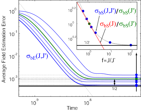
Figure 5: Steady state estimation performance for estimator designed with $J^{\prime}=10^{6}$, and actual spin numbers: $J=J^{\prime}\times[0.5,\,0.75,\,1,\,1.25,\,2,\,10,\,100]$. Other parameters: $\gamma=10^{6}$, $M=10^{4}$, $\gamma_{b}=10^{5}$, $\sigma_{bFree}=1$ (fluctuating field), $\lambda=0.1$ (this is large enough to satisfy large-$\lambda$ limits discussed in text). The inset compares the normalized robust estimation performance (curve) at a particular time, to the ideal performance (line) when $J$ is known.

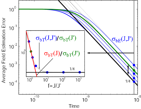
Figure 6: Transient estimation performance for controller designed with $J^{\prime}=10^{6}$, and actual spin numbers: $J=J^{\prime}\times[0.75,\,1,\,1.25,\,2,\,10,\,100,\,1000]$. Other parameters: $\gamma=10^{6}$, $M=10^{4}$, $\gamma_{b}=0$, $\sigma_{bFree}=0$ (constant field), $\lambda=1$. Note that this behavior is valid for $t<1/M=10^{-4}$. The inset compares the normalized robust estimation performance (curve) at a particular time, to the ideal performance (line) when $J$ is known.

On the other hand, when we use precise control the performance improves dramatically. We again simplify the steady state solution with the large $J^{\prime}$ and $\lambda$ assumptions from before, giving

$$\sigma_{bS}(J,J^{\prime}) \rightarrow \left(\frac{1+f}{2f}\right)\sqrt{\frac{2}{\gamma J^{\prime}}}\sigma_{bF}^{3/4}\sigma_{M}^{1/4}$$

$$= \left(\frac{1+f}{2f}\right)\sigma_{bS}(J^{\prime})$$

where $\sigma_{bS}(J,J^{\prime})$ is the steady state controlled error when a plant with $J$ is controlled with a $J^{\prime}$ controller and $\sigma_{bS}(J^{\prime})$ is the error when $J=J^{\prime}$. One simple interpretation of this result is that if we set $J^{\prime}$ to be the minimum of the $J$ distribution ($f>1$) then we never do worse than $\sigma_{bS}(J^{\prime})$ and we never do better than twice as well ($f\rightarrow\infty$). See Figure 5 for a demonstration of this performance.

V.3 Controlled ignorance: transient performance

Now consider measuring constant fields with the wrong assumed $J^{\prime}$. Again, when control is not used, the error saturates at

$$\sigma_{bE}\rightarrow(1-f)^{2}\sigma_{b0}$$

When control is used, the transient performance again improves under certain conditions. The long time transient solution of Eq. (19) is difficult to manage analytically, yet the behavior under certain limits is again simple. For large $\lambda$ and $J^{\prime}$, and for $f>1/2$, we numerically find the transient performance to be approximately

$$\sigma_{bT}(J,J^{\prime}) \rightarrow \left(\frac{f^{2}+2}{4f^{2}-1}\right)\frac{12\sigma_{M}}{\gamma^{2}J^{\prime 2}t^{3}}$$ (27)

$$= \left(\frac{f^{2}+2}{4f^{2}-1}\right)\sigma_{bT}(J^{\prime})$$

where $\sigma_{bT}(J,J^{\prime})$ is the transient controlled error when a plant with $J$ is controlled with a $J^{\prime}$ controller and $\sigma_{bT}(J^{\prime})$ is the error when $J=J^{\prime}$. See Figure 6 for a demonstration of this performance for realistic parameters. As $f\rightarrow\infty$ the $f$-dependent pre-factor saturates at a value of $1/4$. However, as $f\rightarrow 1/2$ then the system takes longer to reach such a simple asymptotic form, and the solution of Eq. (27) becomes invalid.

Accordingly, one robust strategy would be the following. Suppose that the lower bound of the $J$-distribution was known and equal to $J_{min}$. Also assume that $\sigma_{bT}(J_{min})$ represents an acceptable level of performance. In this case, we could simply design our estimator based on $J^{\prime}=J_{min}$ and we would be guaranteed at least the performance $\sigma_{bT}(J_{min})$ and at best the performance $\sigma_{bT}(J_{min})/4$.

This approach would be suitable for experimental situations because typical $J$ distributions are narrow: the difference between $J_{min}$ and $J_{max}$ is rarely greater than an order of magnitude. Thus, the overall sacrifice in performance between the ideal case and the robust case would be small. The estimation performance still suffers because of our ignorance of $J$, but not nearly as much as in the uncontrolled case.

VI Conclusion

The analysis of this paper contained several key steps which should be emphasized. Our first goal was to outline the proper approach to quantum parameter estimation. The second was to demonstrate that reduced representations of the full filtering problem are relevant and convenient because, if a simple representation can be found, then existing classical estimation and control methods can be readily applied. The characteristic that led to this simple description was the approximately Gaussian nature of the problem. Next, we attempted to present basic classical filtering and control methodology in a self-contained, pedagogical format. The results emphasized the inherent trade-offs in simultaneous estimation of distinct, but dynamically coupled, system parameters. Because these methods are potentially critical in any field involving optimal estimation, we consider the full exposition of this elementary example to be a useful resource for future analogous work.

We have also demonstrated the general principle that precision feedback control can make estimation robust to the uncertainty of system parameters. Despite the need to assume that the controller produced a precise cancellation field, this approach deserves further investigation because of its inherent ability to precisely track broadband field signals Geremia et al. (2003a). It is anticipated that these techniques will become more pervasive in the experimental community as quantum systems are refined to levels approaching their fundamental limits of performance.

Appendix A Simplified representation of the plant

In Section II we outlined a general approach to quantum parameter estimation based on the stochastic master equation (SME), but subsequently we derived optimal observer and controller gains from an explicit representation of the plant dynamics (Eq. (6)). This representation appears classical in that the plant state is given by a scalar variable, $z$, rather than a density operator. In this Section we present a derivation of this simplified representation and discuss the equivalence of our approach to the original quantum estimation problem.

From the perspective of quantum filtering theory we will simply show that a Gaussian approximation to the relevant SME can be viewed as a Kalman filter, which in turn induces a simplified representation of the dynamics of the spin state. In this simplified representation the quantum state of the spin system is replaced by a scalar variable, $z$, and $\langle J_{z}\rangle(t)$ is viewed as the optimal estimate of the random process $z(t)$. Equations for $dz(t)$ and its relation to the observed photocurrent $y(t)dt$ are given in Eqs. (30) and (33), which have the convenient property of being formally time-invariant. The technical approach in the main body of the text is then to replace Eq. (28), which is derived from the SME, by a state-space observer derived directly from the simplified model of Eq. (30). By doing so we achieve transparent correspondence with classical estimation and control theory. We should note that the diagrams in Figure 7 indicate signal flows and dependencies in a way that is quite at odds with the quantum filtering perspective. This Figure is meant solely to motivate the simplified model (Eq. (30)) for readers who prefer a more traditional quantum optics perspective, in which the Ito increment in the SME corresponds to optical shot-noise (as opposed to an innovation process derived from the photocurrent) and the SME itself plays the role of a ‘physical’ evolution equation mapping $h(t)$ to $y(t)dt$.

Adopting the latter perspective, let us briefly discuss (with reference to the top diagram in Figure 7) the overall structure of our estimation problem. The physical system that exists in the laboratory (the spins and optical probe beam) acts as a transducer, whose key role in the magnetometry scheme is to imprint a statistical signature of the magnetic field $h(t)$ onto the observable photocurrent, $y(t)dt$. Hence whatever theoretical model we adopt for describing the spin and probe dynamics must provide an accurate description of the mapping from $h(t)$ to $y(t)dt$, as represented by the Plant in Figure 1C. An open-loop estimator, designed on the basis of this plant model, would construct a conditional probability distribution for $h(t)$ based on passive observation of $y(t)dt$. In a closed-loop estimation procedure we would allow the controller to apply compensation fields to the system in order to gain accuracy and/or robustness. In either case, the essential role of the spin-probe (plant) model in the design process is to provide an accurate description of the influence of an arbitrary time-dependent field $h(t)$ on the photocurrent $y(t)dt$. Note that the consideration of arbitrary $h(t)$ subsumes all possible effects of real-time feedback.

Figure 7: Equivalent models for the filtering problem (see discussion at the beginning of Appendix A). Each version can be inserted into the Plant block of Figure 1 C. The filters all presume complete knowledge of $h(t)=b(t)+u(t)$.

Thomsen and co-workers Thomsen et al. (2002) have derived an accurate plant model for our magnetometry problem, in the form of an SME (Eq. (2)). Following a common convention in quantum optics, let us here write this SME and the corresponding photocurrent equation in the form

$$d\rho(t) = -i\,dt[H(h),\rho(t)]+\mathcal{D}[\sqrt{M}J_{z}]\rho(t)\,dt$$

$$+\sqrt{\eta}\mathcal{H}[\sqrt{M}J_{z}]\rho(t)d\bar{W}(t),$$

$$y(t)dt = \langle J_{z}\rangle(t)dt+\sqrt{\sigma_{M}}\,d\bar{W}(t),$$

where $H(h)=\gamma hJ_{y}$ and $\rho(t)$ is the state of the spin system conditioned on the measurement record $y(t)dt$. The quantity $d\bar{W}(t)$ is a Wiener increment that heuristically represents shot-noise in the photodetection process Wiseman and Milburn (1993), and these are to be interpreted as Ito stochastic differential equations. If $h(t)$ and $y(t)dt$ are considered as input and output signals, respectively, this pair of equations jointly implement a plant transfer function as depicted in Figure 7, with $\rho(t)$ taking on the role of the plant state.

For a large spin ensemble, however, $\rho(t)$ will have very high dimension and it would be impractical to utilize the full SME for design purposes. It is straightforward to derive a reduced model by employing a moment expansion for the observable of interest. Extracting the conditional expectation values of the first two moments of $J_{z}$ from SME gives the following scalar stochastic differential equations:

$$d\langle J_{z}\rangle(t) = \gamma\langle J_{x}\rangle(t)h(t)\,dt+\frac{\langle\Delta J_{z}^{2}\rangle(t)}{\sqrt{\sigma_{M}}}d\bar{W}(t)$$

$$d\langle\Delta J_{z}^{2}\rangle(t) = -\frac{\langle\Delta J_{z}^{2}\rangle^{2}(t)}{\sigma_{M}}\,dt$$

$$-i\gamma\langle[\Delta J_{z}^{2},J_{y}]\rangle(t)h(t)\,dt$$

$$+\frac{\langle\Delta J_{z}^{3}\rangle(t)}{\sqrt{\sigma_{M}}}d\bar{W}(t)$$

If the spins are initially fully polarized along $x$ and the spin angle $\sim\langle J_{z}\rangle/\langle J_{x}\rangle$ is kept small (e.g., by active control), then, by using the evolution equation for the $x$ component, we can show $\langle J_{x}\rangle(t)\approx J\exp[-Mt/2]\approx J$ for times $t<1/M$. Making the Gaussian approximation at small times, the third order terms $\langle\Delta J_{z}^{3}\rangle$ and $-i\gamma\langle[\Delta J_{z}^{2},J_{y}]\rangle(t)h(t)$ can be neglected. The Holstein-Primakoff transformation Holstein and Primakoff (1940), commonly used in the condensed matter physics literature, makes it possible to derive this Gaussian approximation as an expansion in $1/J$. Both of the removed terms can be shown to be approximately $1/J\sqrt{J}$ smaller than the retained non-linear term. Additionally, the second removed term will be reduced if $h(t)\approx 0$ by active control.

These approximations give

$$d\langle J_{z}\rangle(t) = \gamma Jh(t)\,dt+\frac{\langle\Delta J_{z}^{2}\rangle(t)}{\sqrt{\sigma_{M}}}d\bar{W}(t)$$ (28)

$$d\langle\Delta J_{z}^{2}\rangle(t) = -\frac{\langle\Delta J_{z}^{2}\rangle^{2}(t)}{\sigma_{M}}\,dt$$ (29)

which constitute a Gaussian, small-time approximation to the full SME that represents the essential dynamics for magnetometry. Note that we can analytically solve

$$\langle\Delta J_{z}^{2}\rangle(t) = \frac{\langle\Delta J_{z}^{2}\rangle(0)\sigma_{M}}{\sigma_{M}+\langle\Delta J_{z}^{2}\rangle(0)t},$$

where $\langle\Delta J_{z}^{2}\rangle(0)=J/2$ for an initial coherent spin state.

At this point we may note that Eqs. (28) and (29) have the algebraic form of a Kalman filter. (This is not at all surprising since the SME, as written in Eq. (2), represents an optimal nonlinear filter for the reduced spin state Belavkin (1999); Verstraete et al. (2001) and our subsequent approximations have enforced both linearity and sufficiency of second-order moments.) Viewed as such, the quantity $\langle J_{z}\rangle(t)$ would represent an optimal (least square) estimate of some underlying variable $z(t)$ based on observation of a signal $d\xi(t)$, and $\langle\Delta J_{z}^{2}\rangle(t)$ would represent the uncertainty (variance) of this estimate. It thus stands to reason that we might be able to simplify our magnetometry model even further if we could find an ‘underlying’ model for the evolution of $z(t)$ and $d\xi(t)$, for which our equations derived from the SME would be the Kalman filter.

It is not difficult to do so, and indeed a very simple model suffices:

$$dz(t) = \gamma Jh(t)dt$$

$$d\xi(t) = z(t)dt+\sqrt{\sigma_{M}}dW(t)$$ (30)

where $dW(t)$ is an Wiener increment that is distinct from (though related to) $d\bar{W}(t)$. In order to match initial conditions with the equations derived from the SME, we should assume that the expected value of $z(t=0)$ is zero and that the variance of our prior distribution for $z(0)$ is $J/2$. Written in canonical form, the Kalman filter for this hypothetical system is then

$$d\tilde{z}(t) = \gamma Jh(t)dt+\frac{\sigma_{zR}(t)}{\sqrt{\sigma_{M}}}\frac{\left[d\xi(t)-\tilde{z}(t)dt\right]}{\sqrt{\sigma_{M}}},$$

$$d\sigma_{zR}(t) = -\frac{\sigma_{zR}^{2}(t)}{\sigma_{M}}\,dt.$$

Here $\tilde{z}(t)$ is the optimal estimate of $z(t)$ and $\sigma_{zR}(t)$ is the variance. We exactly recover the SME model, Eqs. (28) and (29), by the identifications

$$\tilde{z}(t) \leftrightarrow \langle J_{z}\rangle(t)$$

$$\sigma_{zR}(t) \leftrightarrow \langle\Delta J_{z}^{2}\rangle(t)$$

$$\frac{\left[d\xi(t)-\tilde{z}(t)dt\right]}{\sqrt{\sigma_{M}}} \leftrightarrow d\bar{W}(t).$$ (31)

It is important to note that the quantity $\left[d\xi(t)-\tilde{z}dt\right]/\sqrt{\sigma_{M}}$ represents the so-called innovation process of this Kalman filter, and it is thus guaranteed (by least-squares optimality of the filter Oksendal (1998)) to have Gaussian white-noise statistics. Hence we have solid grounds for identifying it with the Ito increment appearing in the SME.

Given this insight, we see that our original magnetometry problem can equivalently be viewed in a way that corresponds to the middle diagram of Figure 7. In this version, we posit the existence of a hidden transducer that imprints statistical information about the magnetic field $h(t)$ onto a signal $d\xi(t)$. A Kalman filter receives this signal, and from it computes an estimate $\tilde{z}(t)$ as well as an innovation process $d\bar{W}(t)$. (Note that as indicated in the diagram, the Kalman filter will only function correctly if it ‘has knowledge of’ the true magnetic field $h(t)$ in the way that a physical system would, but this is not an important point for what follows.) According to the model equations, the Kalman filter then emits the following signal to be received by our photo-detector:

$$y(t)dt = \tilde{z}(t)dt+\sqrt{\sigma_{M}}\,d\bar{W}(t).$$ (32)

Note that $d\bar{W}(t)$ now appears as an internal variable to the Kalman filter, computed from the input signal $d\xi(t)$ and the recursive estimate $\tilde{z}(t)$, while the inherent randomness is referred back to $dW(t)$. Although this may seem like an unnecessarily complicated story, it should be noted that the compound model with $z(t)$ and the Kalman filter predicts an identical transfer function from $h(t)$ to the experimentally-observed signal $y(t)dt$ to that of the equations originally derived from the SME (top diagram in Figure 7). Hence, for the purposes of analyzing and designing magnetometry schemes, these are equivalent models.

Combining several definitions above we find

$$y(t)dt = \tilde{z}(t)dt+\sqrt{\sigma_{M}}\frac{\left[d\xi(t)-\tilde{z}(t)dt\right]}{\sqrt{\sigma_{M}}}$$ (33)

$$= d\xi(t).$$

It thus follows that in the compound model, the Kalman filter actually implements a trivial transfer function and can in fact be eliminated from the diagram. Doing this, we obtain the simplified representation in the bottom diagram of Figure 7. Here the perspective is to pretend that the internal dynamics of the transducing physical system corresponds to the simplified model (Eq. (30)), since we can do so without making any error in our description of the effect of $h(t)$ on the recorded signal. We thus conclude that for the purposes of open- or closed-loop estimation of $h(t)$, filters and controllers can in fact be designed—without loss of performance—using the simplified model (Eq. (30)).

It is interesting to note that $z(t)$ can loosely be interpreted as a ‘classical value’ of the spin projection $J_{z}$. Since the operator $J_{z}$ is a back-action evading observable, the continuous measurement we consider is quantum non-demolition and its backaction on the system state is minimal (conditioning without disturbance). Hence if $h(t)=0$, we may think of the measurement process as gradually ‘collapsing’ the quantum state of the spin system from an initial coherent state towards an eigenstate of $J_{z}$; the hidden variable $z(t)$ in the simplified model Eq. (30) would then represent the eigenvalue corresponding to the ultimate eigenstate, and $\tilde{z}(t)=\langle J_{z}\rangle(t)$ in the Kalman filter would be our converging estimate of it. (Again, this is as expected from the abstract perspective of quantum filtering theory for open quantum systems.) Conditional spin-squeezing in this case can then be understood as nothing more than the reduction of our uncertainty as to the underlying value of $z$ — as we acquire information about $z$ through observation of $d\xi(t)=y(t)dt$, our uncertainty $\sigma_{zR}(t)\leftrightarrow\langle\Delta J_{z}^{2}\rangle(t)$ naturally decreases below its initial coherent-state value of $J/2$. Still, the quantum-mechanical nature of the spin system is not without consequence, as it is known that continuous QND measurement produces entanglement among the spins in the ensemble Stockton et al. (2003).

It seems worth commenting on the fact that Eq. (30) clearly predicts stationary statistics for the photocurrent $y(t)dt$, whereas Eq. (28) contains a time-dependent diffusion coefficient that might color the statistics of $y(t)dt=\langle J_{z}\rangle(t)dt+\sqrt{\sigma_{M}}\,d\bar{W}(t)$. In fact there is no discrepancy. It is possible Wiseman and Milburn (1993) to derive the second order time correlation function of the observed signal $y(t)dt$ directly from the stochastic master Eq. (2),

$$\langle y(t)y(t+\tau)\rangle = (\langle J_{z}(t)J_{z}(t+\tau)\rangle+\langle J_{z}(t+\tau)J_{z}(t)\rangle)/2$$

$$+\frac{1}{4\eta M}\delta(\tau)$$

(This result could also be obtained from the standard input-output theory of quantum optics.) Since the master equation results in linear equations for the mean values $\langle J_{x}(t)\rangle$ and $\langle J_{z}(t)\rangle$ the quantum regression theorem Walls and Milburn (1994) allows the correlation functions $\langle J_{z}(t)J_{z}(t+\tau)\rangle$  and $\langle J_{z}(t+\tau)J_{z}(t)\rangle$ to be calculated explicitly. In this paper we are most interested in the early time evolution for which we obtain the expressions

$$\langle y(t)\rangle=\langle J_{z}(t)\rangle = \gamma bJt+O(t^{2})$$

$$\langle y(0)y(t)\rangle-\langle y(0)\rangle\langle y(t)\rangle = \frac{1}{4\eta M}\delta(t)+\langle\Delta J_{z}^{2}\rangle(0)$$

$$+O(t^{2}).$$

These correlation functions correspond to a white noise signal which is a linear ramp with gradient $\gamma bJ$ with a random offset of variance $\langle\Delta J_{z}^{2}\rangle(0)$, in perfect agreement with our simplified model Eq. (30). If the statistics of $y(t)$ were Gaussian these first and second order moments would be enough to characterize the signal completely, and indeed for sufficiently large $J$ the problem does become effectively Gaussian.

As a final comment we note that the essential step in the above discussion is to observe that the equations for the first and second order moments of the quantum state derived from the stochastic master equation correspond to a Kalman filter for some classical model of a noisy measurement. This correspondence holds for the stochastic master equation corresponding to an arbitrary linear quantum mechanical systems with continuous measurement of observables that are linear combinations of the canonical variables Doherty and Wiseman (2003). In the general case of measurements that are not QND the equivalent classical model will have noise-driven dynamical equations as well as noise on the measured signal. The noise processes driving the dynamics and the measured signal may also be correlated. The case of position measurement of a harmonic oscillator shows all of these features Doherty et al. (1999).

Appendix B Riccati equation solution method

The matrix Riccati equation is ubiquitous in optimal control. Here, following Reid (1972), we show how to reduce the non-linear problem to a set of linear differential equations. Consider the generic Riccati Equation:

$$\frac{d\textbf{V}(t)}{dt}=\textbf{C}-\textbf{D}\textbf{V}(t)-\textbf{V}(t)\textbf{A}-\textbf{V}(t)\textbf{B}\textbf{V}(t)$$

We propose the decomposition:

$$\textbf{V}(t)=\textbf{W}(t)\textbf{U}^{-1}(t)$$

with the linear dynamics

$\begin{bmatrix}\frac{d\textbf{W}(t)}{dt}\\ \frac{d\textbf{U}(t)}{dt}\end{bmatrix}=\begin{bmatrix}-\textbf{D}&\textbf{C}\\ \textbf{B}&\textbf{A}\end{bmatrix}\begin{bmatrix}\textbf{W}(t)\\ \textbf{U}(t)\end{bmatrix}$

It is straightforward to then show that this linearized solution is equivalent to the Riccati equation

$$\frac{d\textbf{V}(t)}{dt} = \frac{d\textbf{W}(t)}{dt}\textbf{U}^{-1}+\textbf{W}(t)\frac{d\textbf{U}^{-1}(t)}{dt}$$

$$= \frac{d\textbf{W}(t)}{dt}\textbf{U}^{-1}(t)+\textbf{W}(t)(-\textbf{U}^{-1}(t)\frac{d\textbf{U}(t)}{dt}\textbf{U}^{-1}(t))$$

$$= (-\textbf{D}\textbf{W}(t)+\textbf{C}\textbf{U}(t))\textbf{U}^{-1}(t)$$

$$-\textbf{W}(t)\textbf{U}^{-1}(t)(\textbf{B}\textbf{W}(t)+\textbf{A}\textbf{U}(t))\textbf{U}^{-1}(t)$$

$$= \textbf{C}-\textbf{D}\textbf{V}(t)-\textbf{V}(t)\textbf{A}-\textbf{V}(t)\textbf{B}\textbf{V}(t)$$

where we have used the identity

$$\frac{d\textbf{U}^{-1}(t)}{dt}=-\textbf{U}^{-1}(t)\frac{d\textbf{U}(t)}{dt}\textbf{U}^{-1}(t)$$

Thus the proposed solution works and the problem can be solved with a linear set of differential equations.

Appendix C Robust control in frequency space

Here we apply traditional frequency-space robust control methods Doyle et al. (1990); Zhou and Doyle (1997) to the classical version of our system. This analysis is different from the treatment in the body of the paper in several respects. First, we assume nothing about the noise sources (bandwidth, strength, etc.). Also, this approach is meant for steady state situations, with the resulting estimator-controller being a constant gain transfer function. The performance criterion we present here is only loosely related to the more complete estimation description above. Despite these differences, this analysis gives a very similar design procedure for the steady state situation.

We proceed as follows with the control system shown in Figure 8, where we label $h(t)=u(t)+b(t)$ as the total field. Consider the usual spin system but ignore noise sources and assume we can measure $z(t)$ directly, so that $z(t)=y(t)$. For small angles of rotation, the transfer function from $h(t)$ to $y(t)$ is an integrator

$$\frac{dy(t)}{dt} = \frac{dz(t)}{dt}=\gamma Jh(t)$$

$$sy(s) = \gamma Jh(s)$$

$$y(s) = P(s)h(s)$$

$$P(s) = \gamma J/s$$

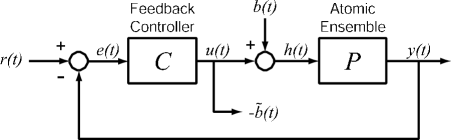
Figure 8: Spin control system with plant transfer function $P(s)=\gamma J/s$. $r(t)$ is the reference signal, which is usually zero. $e(t)$ is the error signal. $u(t)$ is the controller output. $b(t)$ is the external field to be tracked. $h(t)=b(t)+u(t)$ is the total field. $\tilde{b}(t)$ is the field estimate.

Now we define the performance criterion. First notice that the transfer function from the field to be measured $b(t)$ to the total field $h(t)$ is $S(s)$ where

$$h(s) = S(s)b(s)$$

$$S(s) = \frac{1}{1+P(s)C(s)}$$

(Also notice that this represents the transfer function from the reference to the error signal $e(s)=S(s)r(s)$.) Because our field estimate will be $\tilde{b}(t)=-u(t)$, we desire $h(t)$ to be significantly suppressed. Thus we would like $S(s)$ to be small in magnitude (controller gain $|C(s)|$ large) in the frequency range of interest. However, because the gain $|C(s)|$ must physically decrease to zero at high frequencies we must close the feedback loop with adequate phase margin to keep the closed-loop system stable. This is what makes the design of $C(s)$ non-trivial.

Proceeding, we now define a function $W_{1}(s)$ which represents the degree of suppression we desire at the frequency $s=j\omega$. So our controller $C(s)$ should satisfy the following performance criterion

$$\|W_{1}(s)S(s)\|_{\infty} < 1$$

Thus the larger $W_{1}(s)$ becomes, the more precision we desire at the frequency $s$. We choose the following performance function

$$W_{1}(s) = \frac{W_{10}}{1+s/\omega_{1}}$$

such that $\omega_{1}$ is the frequency below which we desire suppression $1/W_{10}$.

Because our knowledge of $J$ is imperfect, we need to consider all plant transfer functions in the range

$$P=\frac{\gamma}{s}\{J_{min}\rightarrow J_{max}\}$$

Our goal is now to find a $C(s)$ that can satisfy the performance condition for any plant in this family. We choose our nominal controller as

$$C_{0}(s) = \frac{\omega_{C}}{\gamma J^{\prime}}$$

So if $J=J^{\prime}$ then the system closes at $\omega_{C}$ (i.e., $|P(i\omega_{C})C_{0}(i\omega_{C})|=1$, whereas in general the system will close at $\omega_{CR}=\omega_{C}\frac{J}{J^{\prime}}$. We choose this controller because $P(s)C(s)$ should be an integrator ($\propto 1/s$) near the closing frequency for optimal phase margin and closed loop stability.

Next we insert this solution into the performance condition. We make the simplifying assumption $\omega_{1}\ll\omega_{C}\frac{J}{J^{\prime}}$ (we will check this later to be self-consistent). Then the optimum of the function is obvious and the condition of Eq. (C) becomes

$$\omega_{1}W_{10}<\omega_{CR}=\omega_{C}\frac{J}{J^{\prime}}$$

We want this condition to be satisfied for all possible spin numbers, so we must have

$$\omega_{1}W_{10}=\min[\omega_{CR}]=\omega_{C}\frac{J_{min}}{J^{\prime}}$$ (34)

Experimentally, we are forced to roll-off the controller at some high frequency that we shall call $\omega_{Q}$. Electronics can only be so fast. Of course, we never want to close above this frequency because the phase margin would become too small, so this determines the maximum $J$ that the controller can reliably handle

$$\omega_{Q}=\max[\omega_{CR}]=\omega_{C}\frac{J_{max}}{J^{\prime}}$$ (35)

Combining Eqs. (34) and (35) we find our fundamental trade-off

$$\omega_{1}W_{10}=\omega_{Q}\frac{J_{min}}{J_{max}}$$ (36)

which is the basic result of this section. Given experimental constraints (such as $J_{min}$, $J_{max}$, and $\omega_{Q}$), it tells us what performance to expect ($1/W_{10}$ suppression) below a chosen frequency $\omega_{1}$.

From Eq. (36), we recognize that the controller gain at the closing frequency needs to be

$$|C|_{C}=\frac{\omega_{C}}{\gamma J^{\prime}}=\frac{\omega_{1}W_{10}}{\gamma J_{min}}=\frac{\omega_{Q}}{\gamma J_{max}}$$

In the final analysis, we do not need to use $J^{\prime}$ and $\omega_{C}$ to parametrize the controller, only the trade-off and the gain. Also, notice that now we can express $\min[\omega_{CR}]=\omega_{1}W_{10}$.

To check our previous assumption

$$\omega_{1} \ll \omega_{C}\frac{J}{J^{\prime}}$$

$$= \omega_{1}W_{10}\frac{J}{J_{min}}$$

which is true if $W_{10}\gg 1$.

Finally, the system will never close below the frequency $\min[\omega_{CR}]$ so we should increase the gain below a frequency $\omega_{H}$ which we might as well set equal to $\min[\omega_{CR}]$. This improves the performance above and beyond the criterion above. Of course we will be forced to level off the gain at some even lower frequency $\omega_{L}$ because infinite DC gain (a real integrator) is unreasonable. So the final controller can be expressed as

$$C(s)=|C|_{C}\frac{1}{1+s/\omega_{Q}}\frac{\omega_{H}(1+s/\omega_{H})}{\omega_{L}(1+s/\omega_{L})}$$

with the frequencies obeying the order

$$\omega_{L} <$$

$$\omega_{H} = \min[\omega_{CR}]=\omega_{1}W_{10}<$$

$$\omega_{CR} = \frac{J}{J_{min}}\omega_{1}W_{10}<$$

$$\omega_{Q} = \max[\omega_{CR}]=\frac{J_{max}}{J_{min}}\omega_{1}W_{10}$$

Notice that the controller now looks like the steady state transfer function in Figure 3 derived from the steady state of the full dynamic filter. (The notation is the same to make this correspondence clear). Here $\omega_{Q}$ was simply stated, whereas there it was a function of $\lambda$ that went to infinity as $\lambda\rightarrow\infty$. Here the high gain due to $\omega_{L}$ and $\omega_{H}$ was added manually, whereas before it came from the design procedure directly.

References

- Armen et al. (2002) M. A. Armen, J. K. Au, J. K. Stockton, A. C. Doherty, and H. Mabuchi, Phys. Rev. Lett 89, 133602 (2002).
- Geremia et al. (2003a) J. M. Geremia, J. K. Stockton, and H. Mabuchi, quant-ph/0309034 (2003a).
- Smith et al. (2002) W. P. Smith, J. E. Reiner, L. A. Orozco, S. Kuhr, and H. M. Wiseman, Phys. Rev. Lett 89, 133601 (2002).
- Morrow et al. (2002) N. V. Morrow, S. K. Dutta, and G. Raithel, Phys. Rev. Lett 88, 093003 (2002).
- Fischer et al. (2002) T. Fischer, P. Maunz, P. W. H. Pinkse, T. Puppe, and G. Rempe, Phys. Rev. Lett 88, 163002 (2002).
- Verstraete et al. (2001) F. Verstraete, A. C. Doherty, and H. Mabuchi, Phys. Rev. A 64, 032111 (2001).
- Gambetta and Wiseman (2001) J. Gambetta and H. M. Wiseman, Phys. Rev. A 64, 042105 (2001).
- Mabuchi (1996) H. Mabuchi, Quantum Semiclass. Opt. 8, 1103 (1996).
- Belavkin (1999) V. Belavkin, Rep. on Math. Phys. 43, 405 (1999).
- Kitagawa and Ueda (1993) M. Kitagawa and M. Ueda, Phys. Rev. A 47, 5138 (1993).
- Kuzmich et al. (2000) A. Kuzmich, L. Mandel, and N. P. Bigelow, Phys. Rev. Lett. 85, 1594 (2000).
- Stockton et al. (2003) J. K. Stockton, J. Geremia, A. C. Doherty, and H. Mabuchi, Phys. Rev. A 67, 022112 (2003).
- Wineland et al. (1994) D. J. Wineland, J. J. Bollinger, W. M. Itano, and D. J. Heinzen, Phys. Rev. A 50, 67 88 (1994).
- Smith et al. (2003) G. A. Smith, S. Chaudhury, and P. S. Jessen, J. Opt. B: Quant. Semiclass. Opt. 5, 323 (2003).
- Kominis et al. (2003) I. K. Kominis, T. W. Kornack, J. C. Allred, and M. Romalis, Nature 422, 596 (2003).
- Budker et al. (2002) D. Budker, W. Gawlik, D. Kimball, S. Rochester, V. Yashchuk, and A. Weiss, Rev. Mod. Phys. 74, 1153 (2002).
- Geremia et al. (2003b) J. M. Geremia, J. K. Stockton, A. C. Doherty, and H. Mabuchi, quant-ph/0306192 (2003b).
- Silberfarb and Deutsch (2003) A. Silberfarb and I. Deutsch, Phys. Rev. A 68, 013817 (2003).
- Thomsen et al. (2002) L. K. Thomsen, S. Mancini, and H. M. Wiseman, Phys. Rev. A 65, 061801 (2002).
- Doherty and Wiseman (2003) A. C. Doherty and H. M. Wiseman, in preparation (2003).
- Jacobs (1996) O. L. R. Jacobs, Introduction to Control Theory (Oxford University Press, New York, 1996), 2nd ed.
- Gardiner (1985) C. W. Gardiner, Handbook of Stochastic Methods (Springer, New York, 1985), 2nd ed.
- Bretthorst (1988) G. L. Bretthorst, Bayesian Spectrum Analysis and Parameter Estimation (Springer Verlag, 1988).
- Wiseman and Milburn (1993) H. M. Wiseman and G. J. Milburn, Phys. Rev. A 47, 642 (1993).
- Holstein and Primakoff (1940) T. Holstein and H. Primakoff, Phys. Rev. 58, 1098 (1940).
- Oksendal (1998) B. Oksendal, Stochastic Differential Equations (Springer Verlag, 1998), 5th ed.
- Walls and Milburn (1994) D. F. Walls and G. J. Milburn, Quantum Optics (Springer Verlag, 1994).
- Doherty et al. (1999) A. C. Doherty, S. M. Tan, A. S. Parkins, and D. F. Walls, Phys. Rev. A 60, 2380 (1999).
- Reid (1972) W. T. Reid, Riccati Differential Equations (Academic Press, New York, 1972).
- Doyle et al. (1990) J. Doyle, B. Francis, and A. Tannenbaum, Feedback Control Theory (Macmillan Publishing Co., 1990).
- Zhou and Doyle (1997) K. Zhou and J. C. Doyle, Essentials of Robust Control (Prentice-Hall, Inc., New Jersey, 1997), 1st ed.