Berry phase in entangled systems: a proposed experiment
with single neutrons

Abstract

The influence of the geometric phase, in particular the Berry phase, on an entangled spin-$\frac{1}{2}$ system is studied. We discuss in detail the case, where the geometric phase is generated only by one part of the Hilbert space. We are able to cancel the effects of the dynamical phase by using the “spin-echo” method. We analyze how the Berry phase affects the Bell angles and the maximal violation of a Bell inequality. Furthermore we suggest an experimental realization of our setup within neutron interferometry.

I Introduction

Entanglement is one of the most profound aspects of quantum mechanics (QM). It occurs in quantum systems that consist of two (or more) parts which can be separated, or typically, in systems whose observables belong to disjoint Hilbert spaces. Its deep meaning has been already realized by Erwin Schrödinger in 1935 in his famous papers on “The present situation of quantum mechanics” Schrodinger . In Schrödinger’s view the whole system is in a definite state whereas the individual parts are not.

In the same year Einstein, Podolsky and Rosen EPR recognized – what nowadays is called “EPR paradox” – that QM exhibits very peculiar correlations between two physically distant parts of the total system. It is possible to predict the outcome of the measurement of one part by looking at the distant part.

About three decades later John S. Bell Bell1964 re-analyzed the “EPR paradox”. He discovered inequalities, commonly known as Bell inequalities (BI), that can be violated by QM but have to be satisfied by (all) local realistic theories BellBook . A violation of a BI demonstrates the presence of entanglement and thus according to Bell’s Theorem the occurrence of nonlocal features in the quantum systems. Generalizations of such inequalities serve as criterion for entanglement or separability BNT .

Experiments with photons (see, e.g., Ref.BertlmannZeilinger for a review) confirm QM with its nonlocality in an impressive way. In the last years there have also been considerable activities to test entangled massive systems in particle physics BertlmannGrimus2001 ; BertlmannHiesmayr2001 ; BertlmannDurstbergerHiesmayr2002 ; BramonNowakowski ; BramonGarbarino ; BramonGarbarinoHiesmayr2003_1 ; GenoveseNoveroPredazzi . Entanglement is the basis for quantum communication and quantum information (see, e.g., Ref.BertlmannZeilinger ) and it became an important issue of investigation nowadays.

Geometric phases such as the Berry phase Berry1 play a considerable role in physics and arise in a quantum system when its time evolution is cyclic and adiabatic. Its deep geometric origin is given by a holonomy of the line bundle of the states where the phase emerges from the integral of the connection (or curvature) of the bundle over the parameter space Simon . The quantum holonomy also appears for mixed states Uhlmann1986 ; DabrowskiGrosse1990 . Generalizations to nonadiabatic evolutions AharonovAnandan and noncyclic and nonunitary settings Pancharatnam ; SamuelBhandari do exist as well as extensions to off-diagonal geometric phases ManiniPistolesi ; FilippSjoqvist . The application of geometric phases in quantum computation has been suggested by several authors ZanardiRasetti ; JonesVedralEkertCastagnoli ; DuanCiracZoller . Experimentally, geometric phases have been tested in various cases, e.g., with photons KwiatChiao ; ChiaoWu ; TomitaChiao , with neutrons HasegawaZawiskyRauchIoffe ; HasegawaLoidlBadurekBaronManiniPistolesiRauch and with atoms WebbGodunSummy .

Whereas the geometric phase in a single particle system is already studied very well, both theoretically and experimentally, its effect on entangled quantum systems is less known. However, there is increasing interest to combine both quantum phenomena, the geometric phase and the entanglement of a system Sjoqvist2000 ; TongKwekOh2003 ; MilmanMosseri2003 ; TongSjoqvistKwekOhEricsson .

In this article we are studying the influence of the Berry phase on the entanglement of a spin-$\frac{1}{2}$ system by considering a BI. The Berry phase is generated by implementing an adiabatically rotating magnetic field into one of the paths of the particles. Our goal is to propose an explicit experimental setup which eliminates the dynamical phase, which would spoil the geometric effect, so that we are sensitive just to the geometric phase. We can achieve this within neutron interferometry BadurekRauchZeilinger ; RauchWerner which is an almost ideal tool to investigate the evolution of a spin-$\frac{1}{2}$ system. In particular, when using a polarized beam BadurekRauchSummhammer we have entanglement between different degrees of freedom, i.e., the spin and the path of the neutron. In this case it is physically rather noncontextuality than locality which is tested experimentally BasuBandyopadhyayKarHome ; HasegawaLoidlBadurekBaronRauch .

Noncontextuality means that the value of an observable does not depend on the experimental context; the measurement of the observable must yield the value independent of other simultaneous measurement. The question is whether the properties of individual parts of a quantum system (or ensemble) do have definite or predetermined values before the act of measurement – a main hypothesis in hidden variable theories. The “no-go theorem” of Bell-Kochen-Specker Bell1966 ; KochenSpecker states that noncontextual theories are incompatible with QM. More precisely, it is in general impossible to assign to an individual quantum system a definite value for each set of observables (see, e.g., Refs.Mermin1993 ; SimonZukowskiWeinfurterZeilinger ).

In our case the observables, which belong to mutually disjoint Hilbert spaces, are the spin and the path of the neutron in the interferometer and we use a BI containing these observables to test noncontextual hidden variable theories versus QM BasuBandyopadhyayKarHome .

II The Berry phase for spin-$\frac{1}{2}$ particles

We concentrate on the spin-$\frac{1}{2}$ system where it is rather simple to implement a geometrical phase and we use Berry’s Berry1 construction for the system evolving adiabatically and cyclically in time.

The scenario is as follows. The particle, without loss of generality moving in $y$-direction, couples to a time dependent magnetic field $\vec{B}(t)$ with unit vector $\vec{n}(\vartheta;t)$ and constant norm $B=|\vec{B}(t)|$. Field $\vec{B}(t)$ rotates adiabatically with an angular velocity $\omega_{0}$ around the $z$-axis under an angle $\vartheta$ (for proper adiabaticity conditions, see Ref.AguiarNemesPeixoto ). The interaction is described by the Hamiltonian

$$H(t)=\frac{\mu}{2}\vec{B}(t)\vec{\sigma}\;,$$ (1)

where the coupling constant is given by $\mu=g\mu_{B}$, the Landé factor $g$ times the Bohr magneton $\mu_{B}=\frac{1}{2}\frac{e}{m}\hbar$.

Consequently, the instantaneous eigenstates of the spin-operator in direction $\vec{n}(\vartheta;t)$ – thus of Hamiltonian (1) – expanded in the $\sigma_{z}$-basis are given by

$$\begin{split}|\Uparrow_{n};t\rangle&=\cos\frac{\vartheta}{2}\;|\Uparrow_{z}\rangle+\sin\frac{\vartheta}{2}\;e^{i\omega_{0}t}\;|\Downarrow_{z}\rangle\\ |\Downarrow_{n};t\rangle&=-\sin\frac{\vartheta}{2}\;|\Uparrow_{z}\rangle+\cos\frac{\vartheta}{2}\;e^{i\omega_{0}t}\;|\Downarrow_{z}\rangle\;.\end{split}$$ (2)

The corresponding time independent energy levels are

$$E_{\pm}=\pm\frac{\mu B}{2}=\pm\hbar\omega_{1}\;,$$ (3)

where $\omega_{1}:=\frac{E_{+}-E_{-}}{2\hbar}=\frac{\mu B}{2\hbar}$ denotes the energy difference of spin $\Uparrow_{n}$ and spin $\Downarrow_{n}$ and represents the characteristic frequency of the system. Let us consider an adiabatic (which means $\frac{\omega_{0}}{\omega_{1}}\ll 1$) and cyclic time evolution for the period $\tau=\frac{2\pi}{\omega_{0}}$ of these eigenstates. Then each eigenstate picks up a phase factor that can be split into a geometrical and dynamical part of the following form

$$\begin{split}\lvert\Uparrow_{n};t=0\rangle\longrightarrow\lvert\Uparrow_{n};t=\tau\rangle&=e^{i\gamma_{+}(\vartheta)}e^{i\theta_{+}}\lvert\Uparrow_{n};t=0\rangle\\ \lvert\Downarrow_{n};t=0\rangle\longrightarrow\lvert\Downarrow_{n};t=\tau\rangle&=e^{i\gamma_{-}(\vartheta)}e^{i\theta_{-}}\lvert\Downarrow_{n};t=0\rangle\;,\end{split}$$ (4)

with

$$\gamma_{+}(\vartheta)=-\pi(1-\cos\vartheta) \gamma_{-}(\vartheta)=-\pi(1+\cos\vartheta)=-\gamma_{+}(\vartheta)-2\pi$$ (5)

$$\theta_{+}=-\frac{1}{\hbar}E_{+}\tau=-2\pi\frac{\omega_{1}}{\omega_{0}} \theta_{-}=+\frac{1}{\hbar}E_{-}\tau=+2\pi\frac{\omega_{1}}{\omega_{0}}=-\theta_{+}\;.$$ (6)

Symbol $\gamma_{\pm}$ denotes the Berry phase which is precisely half of the solid angle $\frac{1}{2}\Omega$ swept out by the magnetic field during the rotation and $\theta_{\pm}$ is the familiar dynamical phase.

Now we are going to eliminate the dynamical effect which would dominate the geometrical one, by using the so called “spin-echo” method. First the propagating particle is subjected to the rotating magnetic field in the direction $\vec{n}(\vartheta)$ for one period and therefore picks up the phases given by Eq.(4). Afterwards the particle passes another rotating field which points in direction $-\vec{n}(\pi-\vartheta)$ again for one period. Then the states change according to

$$\begin{split}\lvert\Uparrow_{n}\rangle\equiv\lvert\Downarrow_{-n}\rangle&\longrightarrow e^{i\gamma_{-}(\pi-\vartheta)}e^{i\theta_{-}}\lvert\Downarrow_{-n}\rangle\equiv e^{i\gamma_{+}(\vartheta)}e^{i\theta_{-}}\lvert\Uparrow_{n}\rangle\\ \lvert\Downarrow_{n}\rangle\equiv\lvert\Uparrow_{-n}\rangle&\longrightarrow e^{i\gamma_{+}(\pi-\vartheta)}e^{i\theta_{+}}\lvert\Uparrow_{-n}\rangle\equiv e^{i\gamma_{-}(\vartheta)}e^{i\theta_{+}}\lvert\Downarrow_{n}\rangle\;.\end{split}$$ (7)

Therefore we get the following net-effect after two rotation-periods

$$\lvert\Uparrow_{n}\rangle\rightarrow e^{2i\gamma_{+}(\vartheta)}\lvert\Uparrow_{n}\rangle\qquad\lvert\Downarrow_{n}\rangle\rightarrow e^{2i\gamma_{-}(\vartheta)}\lvert\Downarrow_{n}\rangle\;,$$ (8)

or for two half-periods of rotation we have

$$\lvert\Uparrow_{n}\rangle\rightarrow e^{i\gamma_{+}(\vartheta)}\lvert\Uparrow_{n}\rangle\qquad\lvert\Downarrow_{n}\rangle\rightarrow e^{i\gamma_{-}(\vartheta)}\lvert\Downarrow_{n}\rangle\;,$$ (9)

where the dynamical effects totally disappear.

III The Berry phase and the entangled state

Let us consider an entangled state of two spin-$\frac{1}{2}$ particles, e.g., the antisymmetric Bell singlet state $\Psi^{(-)}$. One of the particles (e.g., the left side moving particle) interacts twice with the adiabatically rotating magnetic fields as described in Sect.II. Thus only one subspace of the Hilbert space is influenced by the phases.

To locate the Berry phase we decompose the initial Bell singlet state into the eigenstates of the interaction Hamiltonian

$$\lvert\Psi(t=0)\rangle=\lvert\Psi^{(-)}\rangle=\frac{1}{\sqrt{2}}\{\lvert\Uparrow_{n}\rangle_{l}\otimes\lvert\Downarrow_{n}\rangle_{r}-\lvert\Downarrow_{n}\rangle_{l}\otimes\lvert\Uparrow_{n}\rangle_{r}\}\;.$$ (10)

According to our “spin-echo” construction, after one cycle, the state (10) picks up precisely the geometric phase (9)

$$\lvert\Psi(t=\tau)\rangle=\frac{1}{\sqrt{2}}\{e^{i\gamma_{+}}\lvert\Uparrow_{n}\rangle_{l}\otimes\lvert\Downarrow_{n}\rangle_{r}-e^{i\gamma_{-}}\lvert\Downarrow_{n}\rangle_{l}\otimes\lvert\Uparrow_{n}\rangle_{r}\}\;,$$ (11)

which can be rewritten by neglecting an overall phase factor (from now on $\gamma_{+}\equiv\gamma$)

$$\lvert\Psi(t=\tau)\rangle=\frac{1}{\sqrt{2}}\{\lvert\Uparrow_{n}\rangle_{l}\otimes\lvert\Downarrow_{n}\rangle_{r}-e^{-2i\gamma}\lvert\Downarrow_{n}\rangle_{l}\otimes\lvert\Uparrow_{n}\rangle_{r}\}\;.$$ (12)

Increasing the Berry phase $\lvert\gamma\rvert:0\rightarrow\frac{\pi}{2}\rightarrow\pi$, which we achieve by varying the magnetic field angle $\vartheta:0\rightarrow 60^{\circ}\rightarrow 90^{\circ}$, we move continuously from the antisymmetric Bell singlet state $\Psi^{(-)}$ to the symmetric Bell state $\Psi^{(+)}$ and back to $\Psi^{(-)}$.

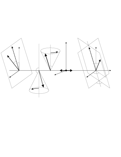
Figure 1: Schematic view of the setup. The vector $\vec{n}$ denotes the quantization direction, $\vec{\alpha}$ and $\vec{\beta}$ are the measurement directions which determine the measurement planes.

As in common Bell experiments we want to measure simultaneously the spin components of the particles on the left and right side, see Fig.1. First we define the projection operator onto an up (+) and down (-) spin state along an arbitrary direction $\vec{\alpha}$

$$P_{\pm}(\vec{\alpha})=\lvert\pm\vec{\alpha}\rangle\langle\pm\vec{\alpha}\rvert$$ (13)

with

$$\begin{split}\lvert+\vec{\alpha}\rangle&=\cos\frac{\alpha_{1}}{2}\lvert\Uparrow_{n}\rangle+\sin\frac{\alpha_{1}}{2}e^{i\alpha_{2}}\lvert\Downarrow_{n}\rangle\\ \lvert-\vec{\alpha}\rangle&=-\sin\frac{\alpha_{1}}{2}\lvert\Uparrow_{n}\rangle+\cos\frac{\alpha_{1}}{2}e^{i\alpha_{2}}\lvert\Downarrow_{n}\rangle\;,\end{split}$$ (14)

where $\alpha_{1}$ denotes the polar angle measured from the $\vec{n}$-direction and $\alpha_{2}$ the azimuthal angle. Then we calculate the joint probability for finding spin-up on the left side under an angle $\vec{\alpha}$ from the quantization axis $\vec{n}$ and spin-up (or spin-down) on the right side under an angle $\vec{\beta}$

$$\begin{split}P(\vec{\alpha}\Uparrow_{n},\vec{\beta}\Uparrow_{n})&=\;\langle\Psi(t=\tau)\rvert P_{+}^{l}(\vec{\alpha})\otimes P_{+}^{r}(\vec{\beta})\lvert\Psi(t=\tau)\rangle\\ &=\;\frac{1}{4}\bigl{(}1-\cos\alpha_{1}\cos\beta_{1}-\cos(\alpha_{2}-\beta_{2}+2\gamma)\sin\alpha_{1}\sin\beta_{1}\bigr{)}\\ &\rightarrow\;\frac{1}{4}\bigl{(}1-\cos(\alpha_{1}-\beta_{1})\bigr{)}\quad\textrm{for}\quad(\alpha_{2}-\beta_{2})\rightarrow-2\gamma\;,\end{split}$$ (15)

$$\begin{split}P(\vec{\alpha}\Uparrow_{n},\vec{\beta}\Downarrow_{n})&=\;\langle\Psi(t=\tau)\rvert P_{+}^{l}(\vec{\alpha})\otimes P_{-}^{r}(\vec{\beta})\lvert\Psi(t=\tau)\rangle\\ &=\;\frac{1}{4}\bigl{(}1+\cos\alpha_{1}\cos\beta_{1}+\cos(\alpha_{2}-\beta_{2}+2\gamma)\sin\alpha_{1}\sin\beta_{1}\bigr{)}\\ &\rightarrow\;\frac{1}{4}\bigl{(}1+\cos(\alpha_{1}-\beta_{1})\bigr{)}\quad\textrm{for}\quad(\alpha_{2}-\beta_{2})\rightarrow-2\gamma\;.\end{split}$$ (16)

Introducing the observable

$$A^{l}(\vec{\alpha})=P_{+}^{l}(\vec{\alpha})-P_{-}^{l}(\vec{\alpha})\;,$$ (17)

and similarly $B^{r}(\vec{\beta})$, we calculate the expectation value of the joint measurement

$$\begin{split}E(\vec{\alpha},\vec{\beta})&=\langle\Psi(t=\tau)\rvert A^{l}(\vec{\alpha})\otimes B^{r}(\vec{\beta})\lvert\Psi(t=\tau)\rangle\\ &=-\cos\alpha_{1}\cos\beta_{1}-\cos(\alpha_{2}-\beta_{2}+2\gamma)\sin\alpha_{1}\sin\beta_{1}\\ &\rightarrow\;-\cos(\alpha_{1}-\beta_{1})\quad\textrm{for}\quad(\alpha_{2}-\beta_{2})\rightarrow-2\gamma\;.\end{split}$$ (18)

We observe that we always can compensate the effect of the Berry phase by simply changing the difference of the azimuthal angles $(\alpha_{2}-\beta_{2})\rightarrow-2\gamma$ of the two measuring directions $\vec{\alpha}$ and $\vec{\beta}$ and regain the familiar expressions without Berry phase.

To test experimentally the influence of a pure geometric phase in the entangled state we have to vary only the opening angle $\vartheta$ of the magnetic field, i.e., the geometry of the setup, which is related to the Berry phase by formula (5). Then we measure expectation value (18) with respect to $\gamma$ at certain fixed directions $\vec{\alpha}$ and $\vec{\beta}$. By rotating the measurement planes by the angle difference $(\alpha_{2}-\beta_{2})=-2\gamma$ the geometric effect is balanced. Experimentally we propose to test this feature within neutron interferometry, see Sect.IV.

When considering a BI to test the local features of the states we find the following behavior, which we want to illustrate by considering the CHSH-inequality (Clauser, Horne, Shimony, Holt) ClauserHorneShimonyHolt , an experimentally testable type of a BI,

$$S\leq 2\;,$$ (19)

where the $S$-function is defined by

$$\begin{split}S(\vec{\alpha},\vec{\alpha}^{\prime},\vec{\beta},\vec{\beta}^{\prime};\gamma)=&\bigl{\lvert}E(\vec{\alpha},\vec{\beta})-E(\vec{\alpha},\vec{\beta}^{\prime})\bigr{\rvert}+\bigl{\lvert}E(\vec{\alpha}^{\prime},\vec{\beta})+E(\vec{\alpha}^{\prime},\vec{\beta}^{\prime})\bigr{\rvert}\\ =&\Bigl{\lvert}-\sin\alpha_{1}\bigl{(}\cos(\alpha_{2}-\beta_{2}+2\gamma)\sin\beta_{1}-\cos(\alpha_{2}-\beta^{\prime}_{2}+2\gamma)\sin\beta^{\prime}_{1}\bigr{)}\\ &\quad-\cos\alpha_{1}\bigl{(}\cos\beta_{1}-\cos\beta^{\prime}_{1}\bigr{)}\Bigr{\rvert}\\ +&\Bigl{\lvert}-\sin\alpha^{\prime}_{1}\bigl{(}\cos(\alpha^{\prime}_{2}-\beta_{2}+2\gamma)\sin\beta_{1}+\cos(\alpha^{\prime}_{2}-\beta^{\prime}_{2}+2\gamma)\sin\beta^{\prime}_{1}\bigr{)}\\ &\quad-\cos\alpha^{\prime}_{1}\bigl{(}\cos\beta_{1}+\cos\beta^{\prime}_{1}\bigr{)}\Bigr{\rvert}\;.\end{split}$$ (20)

Without loss of generality we can eliminate one angle by setting, e.g., $\vec{\alpha}=0$ ($\alpha_{1}=\alpha_{2}=0$), which gives

$$\begin{split}S(\vec{\alpha}^{\prime},\vec{\beta},\vec{\beta}^{\prime};\gamma)=&\Bigl{\lvert}-\sin\alpha^{\prime}_{1}\Bigl{(}\cos(\alpha^{\prime}_{2}-\beta_{2}+2\gamma)\sin\beta_{1}+\cos(\alpha^{\prime}_{2}-\beta^{\prime}_{2}+2\gamma)\sin\beta^{\prime}_{1}\Bigr{)}\\ &-\cos\alpha^{\prime}_{1}(\cos\beta_{1}+\cos\beta^{\prime}_{1})\Bigr{\rvert}+\Bigl{\lvert}-\cos\beta_{1}+\cos\beta^{\prime}_{1}\Bigr{\rvert}\;.\end{split}$$ (21)

We always can reach as maximal value of S the standard value $2\sqrt{2}$. We keep the polar angles $\alpha^{\prime}_{1}$, $\beta_{1}$ and $\beta^{\prime}_{1}$ constant at the Bell angles $\alpha^{\prime}_{1}=\frac{\pi}{2}$, $\beta_{1}=\frac{\pi}{4}$, $\beta^{\prime}_{1}=\frac{3\pi}{4}$ and adjust the azimuthal parts

$$S(\alpha^{\prime}_{2},\beta_{2},\beta^{\prime}_{2};\gamma)=\sqrt{2}+\Bigl{\lvert}-\frac{\sqrt{2}}{2}\Bigl{(}\cos(\alpha^{\prime}_{2}-\beta_{2}+2\gamma)+\cos(\alpha^{\prime}_{2}-\beta^{\prime}_{2}+2\gamma)\Bigr{)}\Bigr{\rvert}\;.$$ (22)

The maximum $2\sqrt{2}$ is reached for $\beta_{2}=\beta^{\prime}_{2}$ and $\alpha^{\prime}_{2}-\beta^{\prime}_{2}=-2\gamma$ (mod $\pi$). For convenience we can choose $\alpha^{\prime}_{2}=0$. The measurement planes on both sides enclose an angle of $2\gamma$, see Fig.1.

On the other hand, keeping the azimuthal angles fixed, e.g., $\alpha_{2}=\alpha^{\prime}_{2}=\beta_{2}=\beta^{\prime}_{2}=0$, the polar Bell angles determined by the maximum of the $S$-function change with respect to the Berry phase $\gamma$. By calculating the derivatives (the extremum condition)

$$\frac{\partial S}{\partial\beta_{1}} = -\sin\beta_{1}\mp\cos\alpha^{\prime}_{1}\sin\beta_{1}\pm\cos(2\gamma)\sin\alpha^{\prime}_{1}\cos\beta_{1}=0$$

$$\frac{\partial S}{\partial\beta^{\prime}_{1}} = \sin\beta^{\prime}_{1}\mp\cos\alpha^{\prime}_{1}\sin\beta^{\prime}_{1}\pm\cos(2\gamma)\sin\alpha^{\prime}_{1}\cos\beta^{\prime}_{1}=0$$ (23)

$$\frac{\partial S}{\partial\alpha^{\prime}_{1}} = \mp\sin\alpha^{\prime}_{1}(\cos\beta_{1}+\cos\beta^{\prime}_{1})\pm\cos(2\gamma)\cos\alpha^{\prime}_{1}(\sin\beta_{1}+\sin\beta^{\prime}_{1})=0\;,$$

the solutions are given by ($\pm$ corresponds to the case either $f_{1}<0$ and $f_{2}<0$ or to $f_{1}<0$ and $f_{2}>0$, when we denote $S=\lvert f_{1}\rvert+\lvert f_{2}\rvert$)

$$\beta_{1} = \pm\arctan(\cos(2\gamma))$$

$$\beta^{\prime}_{1} = \pi-\beta_{1}$$ (24)

$$\alpha^{\prime}_{1} = \frac{\pi}{2}\;,$$

and are plotted in Fig.2 and Fig.3 (of course we may interchange $\beta_{1}\leftrightarrow\beta^{\prime}_{1}$) .

With these angles the $S$-function shows the behavior plotted in Fig.4. We see that the maximal $S$ decreases for $\gamma:0\rightarrow\frac{\pi}{4}$ and touches at $\gamma=\frac{\pi}{4}$ even the limit of the CHSH inequality $S=2$, where we are unable to distinguish between QM and local realistic theories. It increases again to the familiar value $S=2\sqrt{2}$ at $\gamma=\frac{\pi}{2}$, which corresponds to the Bell state $\Psi^{(+)}$.

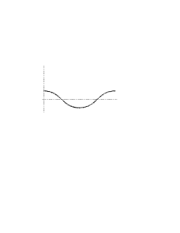
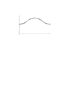
Figure 2: The Bell angles $\beta_{1}$ and $\beta^{\prime}_{1}$ with respect to the Berry phase $\gamma$ for the case $f_{1}<0$ and $f_{2}<0$.

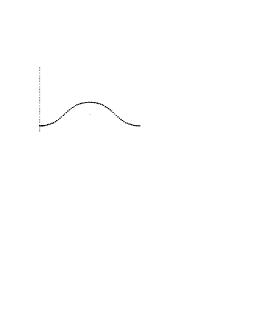
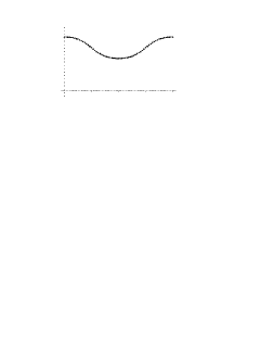
Figure 3: The Bell angles $\beta_{1}$ and $\beta^{\prime}_{1}$ with respect to the Berry phase $\gamma$ for the case $f_{1}<0$ and $f_{2}>0$.

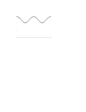
Figure 4: The maximum of the $S$-function (21) with respect to the Berry phase $\gamma$ with the choice of zero azimuthal angles $\alpha^{\prime}_{2}=\beta_{2}=\beta^{\prime}_{2}=0$.

IV Proposed neutron-experiment

Let us now consider how the predicted behavior of $S$ can be measured in practice. In our polarized neutron interferometer experiment the wave function of each neutron is defined over a tensor product of Hilbert spaces which describe the spatial and spin components of the wave function and is entangled analogously to the two spin-$\frac{1}{2}$ system (10)

$$\left|{\Psi}\right\rangle={\frac{1}{\sqrt{2}}}\biggl{\{}\left|{\rm I}\right\rangle\otimes{\left|{s_{\rm I}}\right\rangle-\left|{\rm II}\right\rangle\otimes\left|{s_{\rm II}}\right\rangle}\biggr{\}}\;.$$ (25)

The states $\left|{s_{\rm I}}\right\rangle$ and $\left|{s_{\rm II}}\right\rangle$ denote the spin states of beam-I and -II, as well as $\left|{\rm I}\right\rangle$ and $\left|{\rm II}\right\rangle$ the states in the two beam paths in the interferometer.

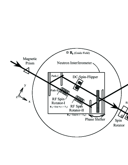
Figure 5: Schematic view of the experimental setup.

A schematic view of the experimental setup is shown in Fig.5. In addition to an auxiliary phase shifter, two radio-frequency (RF) spin-flippers BadurekRauchTuppinger are inserted into one beam path and a direct current (DC) $\pi$-spin-flipper into the other path of the interferometer. The former two flippers enable the neutron spinors to evolve along a particular curve inducing only a geometric phase $\gamma_{B}$ without any dynamical component WaghRakhechaSummhammer ; AllmanKaiserWernerWaghRakhechaSummhammer , see Fig.6. The latter flipper produces the entangled state, like $\left|{\Psi}(t=\tau)\right\rangle$ in Eq.(12). Thus, after the spinor evolution the total wave function is represented by

$$\left|{\Psi(\gamma_{B})}\right\rangle={\frac{1}{\sqrt{2}}}\biggl{\{}\left|{\rm I}\right\rangle\otimes{\left|{\Uparrow_{n}}\right\rangle\rm-\rm{e}^{\mit i\rm\gamma_{B}}\left|{\rm II}\right\rangle\otimes\left|{\Downarrow_{n}}\right\rangle}\biggr{\}}\;,$$ (26)

with the geometrical phase

$$\gamma_{B}=\frac{1}{2}\Omega=\phi_{1}-\phi_{2}.$$ (27)

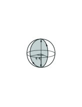
Figure 6: Schematic representation of the spinor evolution with the use of the Poincaré sphere.

Our observables can be decomposed in the following form

$$A^{p}(\chi)=P_{+}^{p}(\chi)-P_{-}^{p}(\chi)\quad\mbox{and}\quad B^{s}(\vec{\delta})=P_{+}^{s}(\vec{\delta})-P_{-}^{s}(\vec{\delta})\;,$$ (28)

where $P_{\pm}^{p}(\chi)$ and $P_{\pm}^{s}(\vec{\delta})$ denote the projection operators onto path and spin states, respectively

$$P_{\pm}^{p}(\chi)=\lvert\pm p\rangle\langle\pm p\,\rvert\quad\mbox{and}\quad P_{\pm}^{s}(\vec{\delta})=\lvert\pm\vec{n}_{\delta}\rangle\langle\pm\vec{n}_{\delta}\rvert\;,$$ (29)

with

$$\begin{split}\lvert+p\rangle&=\cos\frac{\chi}{2}\lvert{\rm I}\rangle+\sin\frac{\chi}{2}\lvert{\rm II}\rangle\qquad\qquad\lvert+\vec{n}_{\delta}\rangle=\cos\frac{\delta_{1}}{2}\lvert\Uparrow_{n}\rangle+\sin\frac{\delta_{1}}{2}e^{i\delta_{2}}\lvert\Downarrow_{n}\rangle\\ \lvert-p\rangle&=-\sin\frac{\chi}{2}\lvert{\rm I}\rangle+\cos\frac{\chi}{2}\lvert{\rm II}\rangle\qquad\quad\lvert-\vec{n}_{\delta}\rangle=-\sin\frac{\delta_{1}}{2}\lvert\Uparrow_{n}\rangle+\cos\frac{\delta_{1}}{2}e^{i\delta_{2}}\lvert\Downarrow_{n}\rangle\;.\end{split}$$ (30)

Once the state $\lvert\Psi(\gamma_{B})\rangle$ is produced joint measurements on the path and spin are performed by choosing the phase shift $\chi$ and the angle $\vec{\delta}$ of the spinor analysis appropriately. Note that $\chi$ and $\vec{\delta}$ play the role of the angles $\vec{\alpha}$ and $\vec{\beta}$ described before in Sect.III.

Experimentally, the joint probabilities are given by the number of counts

$$\begin{split}N_{++}(\chi,\vec{\delta})&=\langle\Psi(\gamma_{B})\rvert P_{+}^{p}(\chi)\otimes P_{+}^{s}(\vec{\delta})\lvert\Psi(\gamma_{B})\rangle\\ N_{+-}(\chi,\vec{\delta})&=\langle\Psi(\gamma_{B})\rvert P_{+}^{p}(\chi)\otimes P_{+}^{s}(\delta_{1}+\pi,\delta_{2})\lvert\Psi(\gamma_{B})\rangle=N_{++}(\chi,(\delta_{1}+\pi,\delta_{2}))\\ N_{-+}(\chi,\vec{\delta})&=\langle\Psi(\gamma_{B})\rvert P_{+}^{p}(\chi+\pi)\otimes P_{+}^{s}(\vec{\delta})\lvert\Psi(\gamma_{B})\rangle=N_{++}(\chi+\pi,\vec{\delta})\\ N_{--}(\chi,\vec{\delta})&=\langle\Psi(\gamma_{B})\rvert P_{+}^{p}(\chi+\pi)\otimes P_{+}^{s}(\delta_{1}+\pi,\delta_{2})\lvert\Psi(\gamma_{B})\rangle=N_{++}(\chi+\pi,(\delta_{1}+\pi,\delta_{2}))\;.\end{split}$$ (31)

Then the expectation value

$$E(\chi,\vec{\delta})=\langle\Psi(\gamma_{B})\rvert A^{p}(\chi)\otimes B^{s}(\vec{\delta})\lvert\Psi(\gamma_{B})\rangle$$ (32)

is experimentally represented by

$$E(\chi,\vec{\delta})=\frac{N_{++}(\chi,\vec{\delta})-N_{+-}(\chi,\vec{\delta})-N_{-+}(\chi,\vec{\delta})+N_{--}(\chi,\vec{\delta})}{N_{++}(\chi,\vec{\delta})+N_{+-}(\chi,\vec{\delta})+N_{-+}(\chi,\vec{\delta})+N_{--}(\chi,\vec{\delta})}\;.$$ (33)

The outcome of (33) coincides with formula (18). Varying the opening angle of the magnetic field – here it is the relative phase of the RF between the two spin rotators – one can demonstrate experimentally the influence of the pure geometric phase of the entangled state on the expectation value (33). Considering the CHSH inequality $S_{\rm max}$ is achieved for $\chi\equiv\alpha_{1}=0$ ($\alpha_{2}=0$), which corresponds to the choice of one path, and $\chi^{\prime}\equiv\alpha^{\prime}_{1}=\frac{\pi}{2}$ ($\alpha^{\prime}_{2}=0$), which means an equal superposition of the states $\lvert{\rm I}\rangle$ and $\lvert{\rm II}\rangle$, whereas the angles $\vec{\delta}\equiv\vec{\beta}$ and $\vec{\delta}^{\prime}\equiv\vec{\beta}^{\prime}$ of the spinor analysis have to be chosen accordingly.

V Summary and conclusion

We have studied the influence of the Berry phase on an entangled spin-$\frac{1}{2}$ system, specifically the case where the Berry phase is generated by one subspace of the system. Due to our special setup with external opposite rotating magnets, the “spin-echo” method, we are able to eliminate the dynamical phase such that only the geometrical part remains. To analyze the effects of the Berry phase we consider the expectation value of spin measurements and test the local feature via a CHSH inequality.

A phase – like our geometrical one – in a pure entangled system does not change the amount of entanglement and therefore not the extent of nonlocality of the system, which is determined by the maximal violation of a BI. Therefore such a phase just affects the Bell angles in a definite way.

We always can achieve the familiar maximum value $2\sqrt{2}$ of the $S$-function by rotating the Bell angles with respect to the Berry phase $\gamma$ by the azimuthal amount $(\alpha_{2}-\beta_{2})=-2\gamma$ as demonstrated in Fig.1. This occurrence of the maximal value is in accordance with Theorems of Horodecki Horodecki2_1996_1 and Gisin Gisin1991 .

On the other hand, keeping the measurement planes fixed the polar Bell angles vary according to formula (III) and the maximum of the $S$-function varies with respect to the Berry phase $\gamma$ as shown in Fig.4. It even touches the boundary of the CHSH inequality at $\gamma=\frac{\pi}{4}$ making any distinction between QM and local realistic theories obsolete for this setup. Other Bell inequalities like Bell’s original one Bell1964 show a similar behavior.

It is our free choice after all whether we rotate the measurement planes accordingly in order to achieve the maximum value $S_{\rm{max}}=2\sqrt{2}$ or keep them fixed at some azimuthal angle and cope with smaller values of $S_{\rm{max}}$. In the second case we show explicitly the dependence of $S_{\rm{max}}$ on the geometric phase.

Entanglement is a quantum property of states defined over a tensor product of Hilbert spaces, no matter what kind of spaces they are. In this sense we certainly can entangle the internal (spin) with the external (space) degrees of freedom of one and the same particle. Then the physical interpretation of a BI, however, differs from the usual nonlocality case and it is the more general concept of contextuality of the states, which is tested, similarly to the Bell-Kochen-Specker Theorem Bell1966 ; KochenSpecker ; Mermin1993 . Noncontextuality here means that the value for the observable spin of the neutron does not depend on the experimental context, i.e., on the other co-measured observable, the path.

Noncontextuality is a rather restrictive demand for a theory, which is incompatible with QM. We propose the experimental test with single particles – the test of noncontextuality versus QM – to be performed within neutron interferometry which is an excellent tool to study the properties of spin-$\frac{1}{2}$ systems. In our case we study both the influence of the Berry phase on entanglement and on contextuality of the states. The neutron experiment which can be easily carried out is in progress.

- (1) E. Schrödinger, Naturwissenschaften 23, 807 (1935); 23, 823 (1935); 23, 844 (1935).
- (2) A. Einstein, B. Podolski and N. Rosen, Phys. Rev. 47, 777 (1935).
- (3) J. S. Bell, Physics 1, 195 (1964).
- (4) J. S. Bell, Speakable and Unspeakable in Quantum Mechanics (Cambridge University Press, Cambridge, 1987).
- (5) R.A. Bertlmann, H. Narnhofer, and W. Thirring, Phys. Rev. A 66, 032319 (2002).
- (6) R. A. Bertlmann and A. Zeilinger (eds.), Quantum [Un]speakables, from Bell to Quantum Information, (Springer Verlag, Heidelberg, 2002).
- (7) R. A. Bertlmann and W. Grimus, Phys. Rev. D 64, 056004 (2001).
- (8) R. A. Bertlmann and B. C. Hiesmayr, Phys. Rev. A 63, 062112 (2001).
- (9) R. A. Bertlmann, K. Durstberger, and B. C. Hiesmayr, Phys. Rev. A 68, 012111 (2003).
- (10) A. Bramon and M. Nowakowski, Phys. Rev. Lett. 83, 1 (1999).
- (11) A. Bramon and G. Garbarino, Phys. Rev. Lett. 88, 04403 (2002).
- (12) A. Bramon, G. Garbarino, and B. C. Hiesmayr, “Quantum marking and quantum erasure for neutral kaons”, quant-ph/0306114 (2003), Phys. Rev. Lett. (in press).
- (13) M. Genovese, C. Novero, and E. Predazzi, Phys. Lett. B 513, 401 (2001).
- (14) M. V. Berry, Proc. R. Soc. Lond. A 392, 45 (1984).
- (15) B. Simon, Phys. Rev. Lett. 51, 2167 (1983).
- (16) A. Uhlmann, Rep. Math. Phys. 24, 229 (1986).
- (17) L. Dabrowski and H. Grosse, Lett. Math. Phys. 19, 205 (1990).
- (18) Y. Aharonov and J. Anandan, Phys. Rev. Lett. 58, 1593 (1987).
- (19) S. Pancharatnam, Proc. Indian Acad. Sci. A 44, 247 (1956).
- (20) J. Samuel and R. Bhandari, Phys. Rev. Lett. 60, 2339 (1988).
- (21) N. Manini and F. Pistolesi, Phys. Rev. Lett. 85, 3067 (2000).
- (22) S. Filipp and E. Sjöqvist, Phys. Rev. Lett. 90, 050403 (2003).
- (23) P. Zanardi and M. Rasetti, Phys. Lett. A 264, 94 (1999).
- (24) J. Jones, V. Vedral, A. Ekert, and G. Castagnoli, Nature 403, 869 (2000).
- (25) L.-M. Duan, J. Cirac, and P. Zoller, Science 292, 1695 (2001).
- (26) P. Kwiat and R. Chiao, Phys. Rev. Lett. 66, 588 (1991).
- (27) R. Chiao and Y.-S. Wu, Phys. Rev. Lett. 57, 933 (1986).
- (28) A. Tomita and R. Chiao, Phys. Rev. Lett. 57, 937 (1986).
- (29) Y. Hasegawa, M. Zawisky, H. Rauch, and A. Ioffe, Phys. Rev. A 53, 2486 (1996).
- (30) Y. Hasegawa, R. Loidl, G. Badurek, M. Baron, N. Manini, F. Pistolesi, and H. Rauch, Phys. Rev. A, 052111 (2002).
- (31) C. L. Webb, R. M. Godun, G. S. Summy, M. K. Oberthaler, P. D. Featonby, C. J. Foot, and K. Burnett, Phys. Rev. A 60, R 1783 (1999).
- (32) E. Sjöqvist, Phys. Rev. A 62, 022109 (2000).
- (33) D. M. Tong, L. C. Kwek, and C. H. Oh, J. Phys. A: Math. Gen. 36, 1149 (2003).
- (34) P. Milman and R. Mosseri, “Topological phase for entangled two-qubit states”, quant-ph/0302202 (2003).
- (35) D. M. Tong, E. Sjöqvist, L. C. Kwek, C. H. Oh, and M. Ericsson, Phys. Rev. A 68, 022106 (2003).
- (36) G. Badurek, H. Rauch, and A. Zeilinger (eds.), Physica B 151, (1988).
- (37) H. Rauch and S. A. Werner, Neutron Interferometry (Oxford Univ. Press, Oxford, 2000).
- (38) G. Badurek, H. Rauch, and J. Summhammer, Physica B 151, 82 (1988).
- (39) S. Basu, S. Bandyopadhyay, G. Kar, and D. Home, Phys. Lett. A 279, 281 (2001).
- (40) Y. Hasegawa, R. Loidl, G. Badurek, M. Baron, and H. Rauch, Nature 425, 45 (2003).
- (41) J. S. Bell, Rev. Mod. Phys. 38, 447 (1966).
- (42) S. Kochen and E. P. Specker, J. Math. Mech. 17, 59 (1967).
- (43) N. D. Mermin, Rev. Mod. Phys. 65, 803 (1993).
- (44) C. Simon, M. Żukowski, H. Weinfurter, and A. Zeilinger, Phys. Rev. Lett. 85, 1783 (2000).
- (45) A. C. Aguiar Pinto, M. C. Nemes, J. G. Peixoto de Faria, and M. T. Thomaz, Am. J. Phys. 68, 955 (2000).
- (46) J. Clauser, M. Horne, A. Shimony, and R. Holt, Phys. Rev. Lett. 23, 880 (1969).
- (47) G. Badurek, H. Rauch, and D. Tuppinger, Phys. Rev. A 34, 2600 (1986).
- (48) A. G. Wagh, V. C. Rakhecha, J. Summhammer, G. Badurek, H. Weinfurter, B. E. Allman, H. Kaiser, K. Hamacher, D. L. Jacobson, and S. A. Werner, Phys. Rev. Lett. 78, 755 (1997).
- (49) B. E. Allman, H. Kaiser, S. A. Werner, A. G. Wagh, V. C. Rakhecha, and J. Summhammer, Phys. Rev. A 56, 4420 (1997).
- (50) R. Horodecki and P. Horodecki, Phys. Lett. A 210, 227 (1996).
- (51) N. Gisin, Phys. Lett. A 154, 201 (1991).