Continuous variable entanglement and quantum state teleportation between optical and macroscopic vibrational modes through radiation pressure

Abstract

We study an isolated, perfectly reflecting, mirror illuminated by an intense laser pulse. We show that the resulting radiation pressure efficiently entangles a mirror vibrational mode with the two reflected optical sideband modes of the incident carrier beam. The entanglement of the resulting three-mode state is studied in detail and it is shown to be robust against the mirror mode temperature. We then show how this continuous variable entanglement can be profitably used to teleport an unknown quantum state of an optical mode onto the vibrational mode of the mirror.

I Introduction

Entanglement is the property possessed by a multipartite quantum systems when it is in a state that cannot be factorized into a product of states or a mixture of these products. In an entangled state the various parties share nonclassical and nonlocal correlations, which are at the basis of the attractive and counterintuitive aspects of quantum mechanics. The study of the properties of entanglement has been recently characterized by an impressive development caused by the discovery that it represents a valuable resource, allowing tasks which are impossible if only separable (unentangled) states are used. In particular, the entanglement shared by two parties significantly increases their communication capabilities. Perhaps the most famous example is quantum state teleportation, i.e. the possibility to send the information contained in a quantum state in a reliable way BEN93 . Other important examples are quantum dense coding, i.e., the possibility to double the classical information transmitted along a channel WIE93 , and the possibility to realize quantum key distribution for cryptography EKE91 . All these schemes for quantum communication have been originally developed for qubits. However, these schemes have been extended quite soon to continuous variable (CV) systems, i.e., quantum systems characterized by observables with a fully continuum spectrum, like position and momentum of a particle, or the quadratures of an e.m. field. In fact, it has been shown, first theoretically VAI94 ; BRA98 and then experimentally FUR98 ; BOW03 how to teleport the quantum state of an e.m. field. Later, most of the quantum communication protocols have been extended to the CV case: dense coding DCOD , quantum key distribution CVCRYP (experimentally demonstrated recently in GRA03 ), and also the possibility to perform CV quantum computation has been discussed CVQCOMP . The interest in CV quantum communication protocols has considerably increased in the last years due to the relative simplicity with which it is possible to generate and manipulate the CV entangled states of the electromagnetic field. The prototype entangled state for CV systems is the simultaneous eigenstate of total momentum and relative distance of two particles, used by Einstein, Podolsky and Rosen (EPR) in their well-known argument EIN35 . The recent development of CV quantum information is mainly due to the fact that its finite-energy version for a two-optical mode system in which the phase and amplitude field quadrature play the role of position and momentum of the particles is just the two-mode squeezed (TMS) state, which can be easily generated by a non degenerate parametric amplifier QO94 . This means that CV entanglement can be generated in a relatively easy way; also its manipulation is not particularly difficult because it requires only linear passive elements as beam splitters and phase shifters. Finally the detection of these entangled state is easy because the Bell measurements (measurements in an entangled basis) in the CV case reduce to homodyne measurements of appropriate quadratures.

However, in any future CV quantum network, it is necessary to have not only light fastly connecting the various nodes, but also physical systems able to store in a stable way and locally manipulate quantum information. This means considering media able to interact and exchange quantum information with optical fields in an efficient way. Moreover this medium should possess entangled states particularly robust and stable against the effects of external noise and imperfections, so that they can be locally manipulated for all the time needed. In the recent literature, various candidates have been proposed for storing CV quantum information. A relatively advanced scheme is the one based on collective atomic spin states POL ; JUL01 , where the involved variable is the total spin, which is actually discrete, but can be safely treated as continuous in the limit of a large number of atoms. In such a case, the presence of entanglement has been already experimentally demonstrated JUL01 . Other schemes are based on mechanical degrees of freedom rather than atomic internal states as, for example, vibrational modes of trapped and cooled ions or atoms PARK , or localized acoustic waves in mirrors PRL02 ; PRL03 . The proposal based on trapped atoms or ions requires the use of traps in conjunction with high-Q cavities, which is technically difficult and for which only preliminary steps have been demonstrated recently CAV . Here we shall discuss in detail the scheme in which CV quantum information is encoded in appropriate acoustic modes of a mirror and for which it has been recently demonstrated the possibility to realize quantum teleportation PRL03 . The radiation pressure of an optical beam incident on a mirror realizes an effective coupling between the electromagnetic modes reflected by the mirror and the vibrational mode of the latter. This coupling can be tuned by varying the intensity of the incident beam. Even though of classical origin, radiation pressure can have important quantum effects: for example, it has been shown that it may be used to generate nonclassical states of both the radiation field FAB ; PRA94 , and the motional degree of freedom of the mirror PRA97 ; marshall .

Moreover, the optomechanical coupling with a vibrating mirror yields an effective nonlinearity for the radiation modes impinging on it. For example optical bistability has been demonstrated in a cavity with a movable mirror bistab . This implies that the mirror, reacting to the radiation pressure, realizes an effective coupling between different optical modes impinging on it. The dynamics of these interacting modes in the case of a driven multi-mode cavity with a movable and perfectly reflecting mirror has been analyzed in detail in Refs. GMT ; ALE ; SILVIA , which studied in particular how CV entanglement between the modes can be generated and characterized. Here, differently from Refs. GMT ; ALE ; SILVIA , we do not consider an optical cavity but only a single mirror, illuminated by an intense and highly monochromatic optical beam. Moreover, we shall not consider only the entanglement between different optical modes but also between the reflected optical modes and the mirror vibrational modes. In particular we shall see that acousto-optical entanglement can be used to teleport the state of an optical mode onto a mirror acoustic mode. This fact opens up the possibility to use a vibrational mode of a mirror as a CV quantum memory and also shows that quantum mechanics can have unexpected manifestations at macroscopic level, involving collective vibrational modes with an effective mass of the order of $\mu$g PRL03 ; marshall .

The paper is organized as follows. In Section II we introduce the system under study, i.e. an isolated mirror illuminated by an intense an quasi-monochromatic light pulse. Under suitable approximations usually satisfied in realistic experimental situations, we derive an effective Hamiltonian for three interacting bosonic modes, the two optical sidebands of the driving mode and one vibrational mode of the mirror. In Section III we exactly solve the three-mode dynamics and in Section IV we perform an extensive study of the CV entanglement between these modes. We shall see that under particular conditions, radiation pressure becomes a source of two-mode squeezing between the two sideband modes. In Section V we then show how the optomechanical entanglement between light and an acoustic mode can be used to teleport a CV state of an optical mode onto the mirror vibrational mode. We shall consider and compare two slightly different protocols, which are both a three-mode adaptation of the protocol by Vaidman, VAI94 and by Braunstein and Kimble BRA98 . Section VI is for concluding remarks.

II The system

The possibility to generate CV entanglement through radiation pressure has been already shown adopting schemes involving a cavity. In Refs. GMT ; ALE ; SILVIA it has been shown how radiation pressure entangles different modes of a driven multi-mode cavity, while Ref. PRL02 has shown how the radiation pressure of an intra-cavity mode entangles the vibrational modes of two oscillating mirrors of a ring cavity. Here we shall consider a simpler scheme with only one vibrating mirror, illuminated by the continuum of travelling electromagnetic modes in free space. This very simple scheme may be useful for quantum communication purposes and moreover it will allow us to study the fundamental aspects of the optomechanical entanglement generated by radiation pressure.

We study for simplicity a perfectly reflecting mirror and consider only the motion and elastic deformations taking place along the spatial direction $x$, orthogonal to its reflecting surface. In the limit of small mirror displacements, and in the interaction picture with respect to the free Hamiltonian of the electromagnetic field and of the mirror displacement field ${\hat{x}({\bf r},t)}$ (${\bf r}$ is the two-dimensional coordinate on the mirror surface), one has the following Hamiltonian PIN99

$${\hat{H}} = -\int\,d^{2}{\bf r}\,{\hat{P}}({\bf r},t){\hat{x}}({\bf r},t)\,,$$ (1)

where ${\hat{P}({\bf r},t)}$ is the radiation pressure force SAM95 . All the continuum of electromagnetic modes with positive longitudinal wave vector $q$, transverse wave vector ${\bf k}$, and frequency $\omega=\sqrt{c^{2}(k^{2}+q^{2})}$ ($c$ being the light speed in the vacuum) contributes to the radiation pressure force. Following Ref. SAM95 , and considering linearly polarized radiation with the electric field parallel to the mirror surface, we have

$${\hat{P}}({\bf r},t) = -\frac{\hbar}{8\pi^{3}}\int d{\bf k}\int dq\int d{\bf k^{\prime}}\int dq^{\prime}\frac{c^{2}qq^{\prime}}{\sqrt{\omega\omega^{\prime}}}({\bf u}_{k}\cdot{\bf u}_{k^{\prime}}){\bf u}_{q}$$ (2)

$$\times \left\{{\hat{a}}({\bf k},q){\hat{a}}({\bf k}^{\prime},q^{\prime})\exp[-i(\omega+\omega^{\prime})t+i({\bf k}+{\bf k}^{\prime})\cdot{\bf r}]\right.$$

$$\left.+{\hat{a}}^{{\dagger}}({\bf k},q){\hat{a}}^{{\dagger}}({\bf k}^{\prime},q^{\prime})\exp[i(\omega+\omega^{\prime})t-i({\bf k}+{\bf k}^{\prime})\cdot{\bf r}]\right.$$

$$\left.+{\hat{a}}({\bf k},q){\hat{a}}^{{\dagger}}({\bf k}^{\prime},q^{\prime})\exp[-i(\omega-\omega^{\prime})t+i({\bf k}-{\bf k}^{\prime})\cdot{\bf r}]\right.$$

$$\left.+{\hat{a}}^{{\dagger}}({\bf k},q){\hat{a}}({\bf k}^{\prime},q^{\prime})\exp[i(\omega-\omega^{\prime})t-i({\bf k}-{\bf k}^{\prime})\cdot{\bf r}]\right\}\,,$$

where ${\hat{a}}({\bf k},q)$ are the continuous mode destruction operators, obeying the commutation relations

$$\left[{\hat{a}}({\bf k},q),{\hat{a}}({\bf k}^{\prime},q^{\prime})\right]=\delta({\bf k}-{\bf k}^{\prime})\delta(q-q^{\prime})\,,$$ (3)

and ${\bf u}_{k}$, ${\bf u}_{q}$ denote dimensionless unit vectors parallel to ${\bf k}$, $q$ respectively.

The mirror displacement ${\hat{x}({\bf r},t)}$ is generally given by a superposition of many acoustic modes PIN99 ; however, a single vibrational mode description can be adopted whenever detection is limited to a frequency bandwidth including a single mechanical resonance. In particular, focused light beams are able to excite Gaussian acoustic modes, in which only a small portion of the mirror, localized at its center, vibrates. These modes have a small waist $w$, a large mechanical quality factor $Q$, a small effective mass $M$ PIN99 , and the simplest choice is to choose the fundamental Gaussian mode with frequency $\Omega$ and annihilation operator $b$, i.e.,

$${\hat{x}}({\bf r},t)=\sqrt{\frac{\hbar}{2M\Omega}}\left[{\hat{b}}e^{-i\Omega t}+{\hat{b}}^{{\dagger}}e^{i\Omega t}\right]\exp(-r^{2}/w^{2})\,.$$ (4)

By inserting Eqs. (2) and (4) into Eq. (1) and integrating over the mirror surface, one gets

$${\hat{H}} = -\frac{\hbar w^{2}}{8\pi^{2}}\sqrt{\frac{\hbar}{2M\Omega}}\int d{\bf k}\int dq\int d{\bf k^{\prime}}\int dq^{\prime}\frac{c^{2}qq^{\prime}}{\sqrt{\omega\omega^{\prime}}}({\bf u}_{k}\cdot{\bf u}_{k^{\prime}}){\bf u}_{q}$$ (5)

$$\times \left\{{\hat{a}}({\bf k},q){\hat{a}}({\bf k}^{\prime},q^{\prime})\exp[-i(\omega+\omega^{\prime})t-({\bf k}+{\bf k}^{\prime})^{2}w^{2}/4]\right.$$

$$\left.+{\hat{a}}^{{\dagger}}({\bf k},q){\hat{a}}^{{\dagger}}({\bf k}^{\prime},q^{\prime})\exp[i(\omega+\omega^{\prime})t-({\bf k}+{\bf k}^{\prime})^{2}w^{2}/4]\right.$$

$$\left.+{\hat{a}}({\bf k},q){\hat{a}}^{{\dagger}}({\bf k}^{\prime},q^{\prime})\exp[-i(\omega-\omega^{\prime})t-({\bf k}-{\bf k}^{\prime})^{2}w^{2}/4]\right.$$

$$\left.+{\hat{a}}^{{\dagger}}({\bf k},q){\hat{a}}({\bf k}^{\prime},q^{\prime})\exp[i(\omega-\omega^{\prime})t-({\bf k}-{\bf k}^{\prime})^{2}w^{2}/4]\right\}\times\left\{{\hat{b}}e^{-i\Omega t}+{\hat{b}}^{{\dagger}}e^{i\Omega t}\right\}\,.$$

The acoustical waist $w$ is typically much larger than optical wavelengths PIN99 , and therefore we can approximate $\exp\left\{-({\bf k}\pm{\bf k^{\prime}})^{2}w^{2}/4\right\}w^{2}/4\pi\simeq\delta({\bf k}\pm{\bf k^{\prime}})$ and then integrate Eq. (5) over ${\bf k^{\prime}}$, obtaining

$${\hat{H}} = -\frac{\hbar}{2\pi}\sqrt{\frac{\hbar}{2M\Omega}}\int d{\bf k}\int dq\int dq^{\prime}\frac{c^{2}qq^{\prime}}{\sqrt{\omega\omega^{\prime}}}$$ (6)

$$\times \left\{-{\hat{a}}({\bf k},q){\hat{a}}(-{\bf k},q^{\prime})\exp[-i(\omega+\omega^{\prime})t]\right.$$

$$\left.-{\hat{a}}^{{\dagger}}({\bf k},q){\hat{a}}^{{\dagger}}(-{\bf k},q^{\prime})\exp[i(\omega+\omega^{\prime})t]\right.$$

$$\left.+{\hat{a}}({\bf k},q){\hat{a}}^{{\dagger}}({\bf k},q^{\prime})\exp[-i(\omega-\omega^{\prime})t]\right.$$

$$\left.+{\hat{a}}^{{\dagger}}({\bf k},q){\hat{a}}({\bf k},q^{\prime})\exp[i(\omega-\omega^{\prime})t]\right\}\times\left\{{\hat{b}}e^{-i\Omega t}+{\hat{b}}^{{\dagger}}e^{i\Omega t}\right\}\,.$$

This is equivalent to consider a very large mirror surface which implies that the transverse momentum of photons is conserved upon reflection.

Here we are considering the time evolution of the continuum of optical modes impinging on the mirror and travelling at the speed of light. The experimental time resolution $\tau$ with which this dynamics is observed is given by the inverse of the detection bandwidth $\Delta\nu_{det}$. Therefore we have to average the Hamiltonian of Eq. (6) over this time resolution $\tau$. We assume $\Delta\nu_{det}\ll\Omega$ which means neglecting all the terms oscillating in time faster than the mechanical frequency $\Omega$, yielding the following replacements in Eq. (6)

$$\exp\left\{\pm i(\omega^{\prime}\pm\omega\pm\Omega)t\right\}\rightarrow\frac{2\pi}{\tau}\delta(\omega^{\prime}\pm\omega\pm\Omega).$$ (7)

Since $\omega$ and $\omega^{\prime}$ are positive and $\Omega$ is much smaller than typical optical frequencies, the two terms $\delta(\omega^{\prime}+\omega\pm\Omega)$ give no contribution, while the other two terms can be rewritten as

$$\frac{2\pi}{\tau}\delta(\omega^{\prime}-\omega\pm\Omega)=2\pi\Delta\nu_{det}\delta(q^{\prime}-\bar{q}_{\pm})\frac{\omega^{\prime}(\bar{q}_{\pm})}{c^{2}\bar{q}_{\pm}},$$ (8)

where $\bar{q}_{\pm}=\sqrt{(\omega\pm\Omega)^{2}/c^{2}-k^{2}}$. Integrating over $q^{\prime}$ we get

$${\hat{H}} = -\hbar\Delta\nu_{det}\sqrt{\frac{\hbar}{2M\Omega}}\int d{\bf k}\int dq\frac{q}{\sqrt{\omega}}\left\{{\hat{a}}({\bf k},q){\hat{a}}^{{\dagger}}\left({\bf k},\bar{q}_{+}\right){\hat{b}}\;\sqrt{\omega+\Omega}+{\hat{a}}({\bf k},q){\hat{a}}^{{\dagger}}\left({\bf k},\bar{q}_{-}\right){\hat{b}}^{{\dagger}}\sqrt{\omega-\Omega}\right.$$ (9)

$$\left.+{\hat{a}}^{{\dagger}}({\bf k},q){\hat{a}}\left({\bf k},\bar{q}_{+}\right){\hat{b}}^{{\dagger}}\sqrt{\omega+\Omega}+{\hat{a}}^{{\dagger}}({\bf k},q){\hat{a}}\left({\bf k},\bar{q}_{-}\right){\hat{b}}\sqrt{\omega-\Omega}\right\}\,,$$

where we have used the fact that $\omega^{\prime}(\bar{q}_{\pm})=\omega\pm\Omega$.

We now consider the situation where the radiation field incident on the mirror is characterized by an intense, quasi-monochromatic, laser field with transversal wave vector ${\bf k_{0}}$, longitudinal wave vector $q_{0}$, cross-sectional area $A$, and power ${\wp}$. Since this component is very intense, it can be treated as classical and one can approximate the bosonic operators ${\hat{a}}({\bf k},q)$ describing the incident field in Eq. (9), with the c-number field

$$\alpha({\bf k},q)=-i\sqrt{\frac{(2\pi)^{3}{\wp}}{\hbar\omega_{0}cA}}\delta({\bf k}-{\bf k_{0}})\delta(q-q_{0})\,,$$ (10)

describing the classical coherent amplitude of the incident field, (it is $\omega_{0}=c\sqrt{{\bf k_{0}}^{2}+q_{0}^{2}}$ in Eq. (10)), while keeping a quantum description for the reflected field ${\hat{a}}({\bf k},\bar{q}_{\pm})$. Inserting Eq. (10) into Eq. (9), the only nonvanishing terms are those involving two back-scattered waves, that is, the sidebands of the driving beam at frequencies $\omega_{0}\pm\Omega$, as described by

$${\hat{H}} = i\hbar\Delta\nu_{det}\sqrt{\frac{\hbar}{2M\Omega}}q_{0}\sqrt{\frac{{\wp}}{\hbar\omega_{0}cA}}\left\{\sqrt{\frac{\omega_{0}+\Omega}{\omega_{0}}}{\hat{a}}^{{\dagger}}\left({\bf k_{0}},\bar{q}_{+}\right){\hat{b}}+\sqrt{\frac{\omega_{0}-\Omega}{\omega_{0}}}{\hat{a}}^{{\dagger}}\left({\bf k_{0}},\bar{q}_{-}\right){\hat{b}}^{\dagger}\right.$$ (11)

$$\left.-\sqrt{\frac{\omega_{0}+\Omega}{\omega_{0}}}{\hat{a}}\left({\bf k_{0}},\bar{q}_{+}\right){\hat{b}}^{\dagger}-\sqrt{\frac{\omega_{0}-\Omega}{\omega_{0}}}{\hat{a}}\left({\bf k_{0}},\bar{q}_{-}\right){\hat{b}}\right\},$$

where now $\bar{q}_{\pm}=\sqrt{(\omega_{0}\pm\Omega)^{2}/c^{2}-k_{0}^{2}}$. The physical process described by this interaction Hamiltonian is very similar to a stimulated Brillouin scattering PER84 , even though in this case the Stokes and anti-Stokes component are back-scattered by the acoustic wave at reflection, and the optomechanical coupling is provided by the radiation pressure and not by the dielectric properties of the mirror (see Fig. 1 for a schematic description).

Figure 1: Schematic description of the system. A laser field at frequency $\omega_{0}$ impinges on the mirror vibrating at frequency $\Omega$. In the reflected field two sideband modes are excited at frequencies $\omega_{1}=\omega_{0}-\Omega$ (Stokes mode) and $\omega_{2}=\omega_{0}+\Omega$ (antiStokes mode).

In practice, either the driving laser beam and the back-scattered modes are never monochromatic, but have a nonzero bandwidth. In general the bandwidth of the back-scattered modes is determined by the bandwidth of the driving laser beam and that of the acoustic mode. However, due to its high mechanical quality factor, the spectral width of the mechanical resonance is negligible (about $1$ Hz) and, in practice, the bandwidth of the two sideband modes $\Delta\nu_{mode}$ coincides with that of the incident laser beam. It is then convenient to consider this nonzero bandwidth to redefine the bosonic operators of the Stokes and anti-Stokes modes to make them dimensionless,

$${\hat{a}}_{1} = 2\pi\sqrt{\frac{2\pi\Delta\nu_{mode}}{cA}}{\hat{a}}\left({\bf k_{0}},\bar{q}_{-}\right)=2\pi\sqrt{\frac{\Delta q}{A}}{\hat{a}}\left({\bf k_{0}},\bar{q}_{-}\right)$$ (12)

$${\hat{a}}_{2} = 2\pi\sqrt{\frac{2\pi\Delta\nu_{mode}}{cA}}{\hat{a}}\left({\bf k_{0}},\bar{q}_{+}\right)=2\pi\sqrt{\frac{\Delta q}{A}}{\hat{a}}\left({\bf k_{0}},\bar{q}_{+}\right),$$ (13)

so that Eq.(11) reduces to an effective Hamiltonian

$${\hat{H}}_{eff}=-i\hbar\chi({\hat{a}}_{1}{\hat{b}}-{\hat{a}}^{{\dagger}}_{1}{\hat{b}}^{{\dagger}})-i\hbar\theta({\hat{a}}_{2}{\hat{b}}^{{\dagger}}-{\hat{a}}^{{\dagger}}_{2}{\hat{b}})\,,$$ (14)

where the couplings $\chi$ and $\theta$ are given by

$$\chi = q_{0}\Delta\nu_{det}\sqrt{\frac{\hbar}{2M\Omega}}\sqrt{\frac{{\wp}}{\Delta\nu_{mode}\hbar\omega_{0}}}\sqrt{\frac{\omega_{0}-\Omega}{\omega_{0}}}=\cos\phi_{0}\sqrt{\frac{{\wp}\Delta\nu_{det}^{2}(\omega_{0}-\Omega)}{2M\Omega c^{2}\Delta\nu_{mode}}}$$ (15)

$$\theta = \chi\sqrt{\frac{\omega_{0}+\Omega}{\omega_{0}-\Omega}},$$ (16)

with $\phi_{0}=\arccos(cq_{0}/\omega_{0})$, is the angle of incidence of the driving beam. It is possible to verify that with the above definitions, the Stokes and anti-Stokes annihilation operators $\hat{a}_{1}$ and $\hat{a}_{2}$ satisfy the usual commutation relations $\left[\hat{a}_{i},\hat{a}_{j}^{\dagger}\right]=\delta_{i,j}$.

III System dynamics

Eq. (14) shows that the radiation pressure of an intense monochromatic laser beam incident on a mirror generates an effective coupling between a given vibrational mode of the mirror and the two first optical sideband modes induced by the vibrations. One has a system of three, bilinearly coupled, bosonic modes, which is formally equivalent to a system of three optical modes interacting through coupled parametric down-conversion and up-conversion with simultaneous phase matching. This system has been experimentally studied in the classical domain in rabin , while the quantum photon statistics has been determined in Ref. smithers . More recently, the same optical system has been proposed for the implementation of symmetrical and asymmetrical quantum telecloning in paris1 . The same three mode dynamics has also been studied within a cavity configuration wong , where however the dissipation associated with cavity losses significantly changes the dynamics. Finally, a similar Hamiltonian describes also the interaction of two atomic modes with opposite momentum in a Bose-Einstein condensate with an off-resonant optical mode scattered by it, and its quantum dynamics has been recently discussed in paris2 .

Eq. (14) contains two interaction terms: the first one, between modes ${\hat{a}}_{1}$ and ${\hat{b}}$, is a parametric-type interaction leading to squeezing in phase space QO94 , and it is able to generate the EPR-like entangled state which has been used in the CV teleportation experiment of Ref. FUR98 . The second interaction term, between modes ${\hat{a}}_{2}$ and ${\hat{b}}$, is a beam-splitter-type interaction QO94 . This purely Hamiltonian description satisfactorily reproduces the dynamics as long as the dissipative coupling of the mirror vibrational mode with its environment is negligible. This happens for vibrational modes with a high-Q mechanical quality factor. In this case we can consider an interaction time, i.e., a time duration of the incident laser pulse, much smaller than the relaxation time of the vibrational mode (which can be of order of one second TIT99 ).

The Hamiltonian (14) leads to a system of linear Heisenberg equations, namely

$$\dot{\hat{a}}_{1} = \chi{\hat{b}}^{{\dagger}}\,,$$ (17)

$$\dot{\hat{b}} = \chi{\hat{a}}_{1}^{{\dagger}}-\theta{\hat{a}}_{2}\,,$$ (18)

$$\dot{\hat{a}}_{2} = \theta{\hat{b}}\,.$$ (19)

The solutions read

$${\hat{a}}_{1}(t) = \frac{1}{\Theta^{2}}\left[\theta^{2}-\chi^{2}\cos\left(\Theta t\right)\right]{\hat{a}}_{1}(0)+\frac{\chi}{\Theta}\sin\left(\Theta t\right){\hat{b}}^{{\dagger}}(0)-\frac{1}{\Theta^{2}}\left[\chi\theta-\chi\theta\cos\left(\Theta t\right)\right]{\hat{a}}_{2}^{{\dagger}}(0)\,,$$ (20)

$${\hat{b}}(t) = -\frac{\chi}{\Theta}\sin\left(\Theta t\right){\hat{a}}_{1}^{{\dagger}}(0)+\cos\left(\Theta t\right){\hat{b}}(0)-\frac{\theta}{\Theta}\sin\left(\Theta t\right){\hat{a}}_{2}(0)\,,$$ (21)

$${\hat{a}}_{2}(t) = \frac{1}{\Theta^{2}}\left[\chi\theta-\chi\theta\cos\left(\Theta t\right)\right]{\hat{a}}_{1}^{{\dagger}}(0)-\frac{\theta}{\Theta}\sin\left(\Theta t\right){\hat{b}}(0)-\frac{1}{\Theta^{2}}\left[\chi^{2}-\theta^{2}\cos\left(\Theta t\right)\right]{\hat{a}}_{2}(0)\,,$$ (22)

where $\Theta=\sqrt{\theta^{2}-\chi^{2}}$.

On the other hand, the system dynamics can be easily studied also through the normally ordered characteristic function $\Phi(\mu,\nu,\zeta)$ QO94 , where $\mu,\nu,\zeta$ are the complex variables corresponding to the operators ${\hat{a}}_{1},{\hat{b}},{\hat{a}}_{2}$ respectively. From the Hamiltonian (14) the dynamical equation for $\Phi$ results

$${\dot{\Phi}} = \chi\left(\mu\nu+\mu^{*}\nu^{*}-\mu^{*}\frac{\partial}{\partial\nu}-\mu\frac{\partial}{\partial\nu^{*}}-\nu^{*}\frac{\partial}{\partial\mu}-\nu\frac{\partial}{\partial\mu^{*}}\right)\Phi$$ (23)

$$+\theta\left(\zeta^{*}\frac{\partial}{\partial\nu^{*}}+\zeta\frac{\partial}{\partial\nu}-\nu^{*}\frac{\partial}{\partial\zeta^{*}}-\nu\frac{\partial}{\partial\zeta}\right)\Phi\,,$$

with the initial condition

$$\Phi(t=0)=\exp\left[-\overline{n}|\nu|^{2}\right]\,,$$ (24)

corresponding to the vacuum for the modes ${\hat{a}}_{1}$, ${\hat{a}}_{2}$ and to a thermal state for the mode ${\hat{b}}$. The latter is characterized by an average number of excitations $\overline{n}=[\coth(\hbar\Omega/2k_{B}T)-1]/2$, $T$ being the equilibrium temperature and $k_{B}$ the Boltzmann constant. Since the initial condition is a Gaussian state of the three-mode system, and the system is linear, the joint state of the whole system at time $t$ is still Gaussian, with characteristic function

$$\Phi=\exp\left[-{\cal A}|\mu|^{2}-{\cal B}|\nu|^{2}-{\cal E}|\zeta|^{2}+{\cal C}\mu\nu+{\cal C}\mu^{*}\nu^{*}+{\cal F}\mu\zeta+{\cal F}\mu^{*}\zeta^{*}+{\cal D}\nu\zeta^{*}+{\cal D}\nu^{*}\zeta\right]\,,$$ (25)

where

$${\cal A}(t) = \frac{1}{2(r^{2}-1)^{2}}\left\{\left[1-\cos\left(2\Theta t\right)\right]\left[\overline{n}(r^{2}-1)-1\right]\right.$$ (26)

$$\left.+4r^{2}\left[1-\cos\left(\Theta t\right)\right]\right\}\,,$$

$${\cal B}(t) = \frac{1}{2(r^{2}-1)}\left\{\left[1+\cos\left(2\Theta t\right)\right]\overline{n}(r^{2}-1)+1-\cos\left(2\Theta t\right)\right\}\,,$$ (27)

$${\cal C}(t) = \frac{1}{2(r^{2}-1)^{3/2}}\left\{2r^{2}\sin\left(\Theta t\right)\right.$$ (28)

$$\left.+\left[\overline{n}(r^{2}-1)-1\right]\sin\left(2\Theta t\right)\right\}\,,$$

$${\cal D}(t) = \frac{-r}{2(r^{2}-1)^{3/2}}\left\{2\sin\left(\Theta t\right)+\left[\overline{n}(r^{2}-1)-1\right]\sin\left(2\Theta t\right)\right\}\,,$$ (29)

$${\cal E}(t) = \frac{r^{2}}{2(r^{2}-1)^{2}}\left\{\left[1-\cos\left(2\Theta t\right)\right]\left[\overline{n}(r^{2}-1)-1\right]\right.$$ (30)

$$\left.+4\left[1-\cos\left(\Theta t\right)\right]\right\}\,,$$

$${\cal F}(t) = \frac{r}{2(r^{2}-1)^{2}}\left\{\left[1-\cos\left(2\Theta t\right)\right]\left[\overline{n}(r^{2}-1)-1\right]\right.$$ (31)

$$\left.+2(1+r^{2})\left[1-\cos\left(\Theta t\right)\right]\right\}\,,$$

and $r=\theta/\chi=\left[(\omega_{0}+\Omega)/(\omega_{0}-\Omega)\right]^{1/2}$. Eqs. (26-31) show that the system dynamics depends upon three dimensionless parameters: the initial vibrational mean thermal excitation number $\bar{n}$; the scaled time $t^{\prime}\equiv\Theta t$; the ratio between coupling constants $r$, which depends only upon the ratio between the vibrational frequency and the optical driving frequency and it is always very close to one. Since within the approximations introduced in the preceding Section, the system can be described as a closed system of three interacting oscillators, the resulting dynamics is periodic, with period $2\pi$ for the scaled variable $t^{\prime}$. For this reason we shall consider only $0\leq t^{\prime}\leq 2\pi$ in the following.

The state of the system can be equivalently described also in terms of its correlation matrix (CM) $V$, defined by $V_{ij}=\langle\Delta\hat{\xi}_{i}\Delta\hat{\xi}_{j}+\Delta\hat{\xi}_{j}\Delta\hat{\xi}_{i}\rangle/2$, where $\Delta\hat{\xi}_{i}=\hat{\xi}_{i}-\langle\hat{\xi}_{i}\rangle$ and $\hat{\xi}$ denotes the following vector of quadratures, $\hat{\xi}=(\hat{X}_{1},\hat{P}_{1},\hat{X}_{b},\hat{P}_{b},\hat{X}_{2},\hat{P}_{2})$, defined by $\hat{X}_{k}=(\hat{a}_{k}+\hat{a}_{k}^{\dagger})/\sqrt{2}$, $\hat{P}_{k}=(\hat{a}_{k}-\hat{a}_{k}^{\dagger})/i\sqrt{2}$ ($k=1,2$), and $\hat{X}_{b}=(\hat{b}+\hat{b}^{\dagger})/\sqrt{2}$, $\hat{P}_{b}=(\hat{b}-\hat{b}^{\dagger})/i\sqrt{2}$. In fact, the CM of a Gaussian state is directly connected with the symmetrically ordered correlation function $\Phi_{sym}(\mu,\nu,\zeta)=\exp\left\{-(|\mu|^{2}+|\nu|^{2}+|\zeta|^{2})/2\right\}\Phi(\mu,\nu,\zeta)$. In the present case, the three mode system is at all times a zero-mean Gaussian state and therefore this connection can be written as

$$\Phi_{sym}(\xi)=\exp\left\{-\sum_{i,j=1}^{6}\xi_{i}V_{ij}\xi_{j}\right\},$$ (32)

where $\xi$ is the six-dimensional vector of phase space coordinates corresponding to the quadratures $\hat{\xi}$. Using Eq. (25), one gets

0𝒜+120−𝒞0−ℱ𝒞0ℬ+120−𝒟00−𝒞0ℬ+120−𝒟ℱ0−𝒟0ℰ+1200−ℱ0−𝒟0ℰ+12).𝑉fragments 0fragmentsA120fragmentsC0fragmentsF𝒞0fragmentsB120fragmentsD00fragmentsC0fragmentsB120fragmentsDℱ0fragmentsD0fragmentsE1200fragmentsF0fragmentsD0fragmentsE12V=\left(\begin{tabular}[c]{cc|cc|cc}${\cal A}+\frac{1}{2}$&$0$&${\cal C}$&$0$&${\cal F}$&$0$\\ $0$&${\cal A}+\frac{1}{2}$&$0$&$-{\cal C}$&$0$&$-{\cal F}$\\ \hline\cr${\cal C}$&$0$&${\cal B}+\frac{1}{2}$&$0$&$-{\cal D}$&$0$\\ $0$&$-{\cal C}$&$0$&${\cal B}+\frac{1}{2}$&$0$&$-{\cal D}$\\ \hline\cr${\cal F}$&$0$&$-{\cal D}$&$0$&${\cal E}+\frac{1}{2}$&$0$\\ $0$&$-{\cal F}$&$0$&$-{\cal D}$&$0$&${\cal E}+\frac{1}{2}$\\ \end{tabular}\right)\;.

+A120C0F0+A120C0F0 (33)

IV Separability properties of the tripartite CV system

In the preceding Section we have completely determined the dynamics of the system and these results allow us to perform a complete characterization of the separability properties of this tripartite CV system. For systems composed of more than two parties, one has many “types” of entanglement due to the many ways in which the different subsystems may be entangled with each other. As a first task we classify the entanglement possessed by the system as a function of the various parameters.

IV.1 Entanglement classification

Following the scheme introduced in dur , one has five different entanglement classes for a tripartite system:

Class 1. Fully inseparable states, i.e. not separable for any grouping of the parties.

Class 2. One-mode biseparable states, which are separable if two of the parties are grouped together, but inseparable with respect to the other groupings.

Class 3. Two-mode biseparable states, which are separable with respect to two of the three possible bipartite splits but inseparable with respect to the third.

Class 4. Three-mode biseparable states, which are separable with respect to all three bipartite splits but cannot be written as a mixture of tripartite product states.

Class 5. Fully separable states, which can be written as a mixture of tripartite product states.

The state of our tripartite system is easy to determine at some specific time instants. Due to periodicity, at $t^{\prime}=0,2\pi$ the state is simply the chosen initial state, i.e. the tripartite product of a thermal state for the mirror and the vacuum state for the Stokes and the antiStokes sideband modes. Therefore at these isolated time instants the state belongs to class $5$ simply because of the assumed fully separable initial state. The state of the system is easy to determine also at $t^{\prime}=\pi$, i.e. just in the middle of its periodic evolution. In fact, choosing $t^{\prime}=\pi$ in Eq. (33), the CM becomes

04​r2(r2−1)2+12000−2​r​(r2+1)(r2−1)200n¯+12000000n¯+12002​r​(r2+1)(r2−1)20004​r2(r2−1)2+1200−2​r​(r2+1)(r2−1)20004​r2(r2−1)2+12)=V12T​M​S⊕Vbn¯,𝑉superscript𝑡′𝜋fragments 0fragments4superscript𝑟2superscriptsuperscript𝑟21212000fragments2𝑟superscript𝑟21superscriptsuperscript𝑟21200fragments¯𝑛12000000fragments¯𝑛1200fragments2𝑟superscript𝑟21superscriptsuperscript𝑟212000fragments4superscript𝑟2superscriptsuperscript𝑟2121200fragments2𝑟superscript𝑟21superscriptsuperscript𝑟212000fragments4superscript𝑟2superscriptsuperscript𝑟21212direct-sumsuperscriptsubscript𝑉12𝑇𝑀𝑆superscriptsubscript𝑉𝑏¯𝑛V\left(t^{\prime}=\pi\right)=\left(\begin{tabular}[c]{cc|cc|cc}$\frac{4r^{2}}{\left(r^{2}-1\right)^{2}}+\frac{1}{2}$&$0$&$0$&$0$&$\frac{2r\left(r^{2}+1\right)}{\left(r^{2}-1\right)^{2}}$&$0$\\ $0$&$\frac{4r^{2}}{\left(r^{2}-1\right)^{2}}+\frac{1}{2}$&$0$&$0$&$0$&$-\frac{2r\left(r^{2}+1\right)}{\left(r^{2}-1\right)^{2}}$\\ \hline\cr$0$&$0$&$\bar{n}+\frac{1}{2}$&$0$&$0$&$0$\\ $0$&$0$&$0$&$\bar{n}+\frac{1}{2}$&$0$&$0$\\ \hline\cr$\frac{2r\left(r^{2}+1\right)}{\left(r^{2}-1\right)^{2}}$&$0$&$0$&$0$&$\frac{4r^{2}}{\left(r^{2}-1\right)^{2}}+\frac{1}{2}$&$0$\\ $0$&$-\frac{2r\left(r^{2}+1\right)}{\left(r^{2}-1\right)^{2}}$&$0$&$0$&$0$&$\frac{4r^{2}}{\left(r^{2}-1\right)^{2}}+\frac{1}{2}$\end{tabular}\right)=V_{12}^{TMS}\oplus V_{b}^{\bar{n}},

+4r2(-r21)2120002r(+r21)(-r21)20+4r2(-r21)2120002r(+r21)(-r21)20 (34)

where $V_{12}^{TMS}$ is the $4\times 4$ CM of a TMS state for the two optical sidebands and $V_{b}^{\bar{n}}$ is the one-mode CM of a thermal state with mean excitation number $\bar{n}$ for the mirror. Therefore at half period the mirror vibrational mode factorizes from the two optical modes which are instead in a TMS state with a two-mode squeezing parameter given by $\sinh^{-1}\left[2r(r^{2}+1)/(r^{2}-1)^{2}\right]$. This means that at $t^{\prime}=\pi$ the state is a one-mode biseparable state, i.e. belongs to class $2$, for any value of the mirror temperature and of the ratio $r$.

It is important to notice that the reduced state of the two sideband modes at $t^{\prime}=\pi$ is independent of the mirror temperature and, being a TMS state, its entanglement can be arbitrarily increased by increasing the squeezing parameter, which in this case is realized by letting $r\to 1\Leftrightarrow\Omega/\omega_{0}\to 0$. This means that when the interaction time, i.e. the duration of the driving laser pulse, is carefully chosen so that $t^{\prime}=\pi$, the two reflected sideband modes are entangled in the same way as the twin beams at the output of a nondegenerate parametric amplifier and this entanglement is insensitive with respect to the mirror temperature. Therefore, under appropriate conditions, radiation pressure becomes an alternative tool for the generation of CV entanglement between optical modes JOPB .

For interaction times different from the above special cases, we can still determine the entanglement class of the system state by applying the results of Ref. entcirac , which has provided a necessary and sufficient criterion for the determination of the class in the case of tripartite CV Gaussian states and which is directly computable. This classification criterion is mostly based on the nonpositive partial transposition (NPT) criterion proved in entwerner , which is necessary and sufficient for $1\times N$ bipartite CV Gaussian states. The NPT criterion of entwerner can be expressed in terms of the symplectic matrix

$${\cal J}=\bigoplus_{i=1}^{3}J_{i},\;\;\;\;\;\;J_{i}=\left(\begin{array}[c]{cc}0&1\\ -1&0\end{array}\right)\;\;\;\;\;{\rm i=1,2,3}$$ (35)

expressing the commutation rules between the canonical coordinates $[\hat{\xi}_{\alpha},\hat{\xi}_{\beta}]=i{\cal J}_{\alpha\beta}$, and of the partial transposition transformation $\Lambda_{k}$, acting on system $k$ only. Transposition is equivalent to time reversal and therefore in phase space is equivalent to change the sign of the momentum operators, i.e. $\Lambda_{k}(\ldots,X_{k},P_{k},\ldots)=(\ldots,X_{k},-P_{k},\ldots)$. The NPT criterion states that a $1\times N$ CV Gaussian state is separable if and only if the “test matrix” $\tilde{V}_{k}=\Lambda_{k}V\Lambda_{k}+i{\cal J}/2\geq 0$. Therefore by evaluating the sign of the eigenvalues of the three matrices $\tilde{V}_{k}$, $k=1,2,b$ and using the NPT criterion one can discriminate states belonging to class $1$ (none of the three matrices $\tilde{V}_{k}$ is positive), class $2$ (only one of the $\tilde{V}_{k}$ is positive), and class $3$ (two of the $\tilde{V}_{k}$ are positive). When all the $\tilde{V}_{k}$ are positive, NPT criterion is not able to distinguish between class $4$ and $5$ and a specific criterion for this case has been derived in entcirac . However in the present case this latter result is not needed and the entanglement classification is simple also for interaction times $t^{\prime}\neq m\pi$ (integer $m$). In fact, denoting with $\eta_{j}(t^{\prime},r,\bar{n})$ the minimum eigenvalue of $\tilde{V}_{j}$, we have numerically checked that $\eta_{j}(t^{\prime},r,\bar{n})$ is always negative for $j=1,2,b$, $\forall t^{\prime}\neq m\pi$ and for a very large range of $\bar{n}$ and $r$ footn , and therefore the state of the system is fully inseparable. For example, in the case $r=1+2.5\times 10^{-7}$, $\forall t^{\prime}\neq m\pi$ we have $\eta_{1}(t^{\prime},\bar{n})\simeq\eta_{2}(t^{\prime},\bar{n})\simeq-0.5$ independent of $\bar{n}$, with only $\eta_{b}(t^{\prime},\bar{n})$ significantly depending on the mirror temperature. By taking the logarithm of the modulus of this negative eigenvalues as a measure of entanglement (a sort of logarithmic negativity loga ), this means that only the entanglement between the vibrational mode and the subsystem formed by the two optical modes is sensitive to temperature, while the entanglement between one sideband mode and the other two modes is not. This example of logarithmic negativity $\log_{10}\left\{|\eta_{b}(t^{\prime})|\right\}$ is shown in Fig. 2 for different values of $\bar{n}$. As expected, the entanglement between the mirror mode and the two optical mode decreases with increasing temperature. We conclude that our tripartite state is almost everywhere fully entangled (class 1) except for the isolated time instants $t^{\prime}=2k\pi$ when it is fully separable (class 5) and at instants $t^{\prime}=(2k+1)\pi$ when it is one-mode biseparable (class 2).

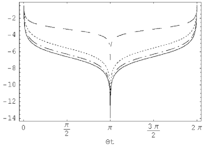
Figure 2: Logarithmic negativity $\log_{10}\left\{|\eta_{b}(t^{\prime})|\right\}$ (see text) vs the scaled time $t^{\prime}=\Theta t$. The values of other parameters are: $r=1+2.5\times 10^{-7}$ and $\bar{n}=0$ dashed line, $\bar{n}=10^{-1}$ dotted line, $\bar{n}=1$ dotted-dashed line, $\bar{n}=10^{7}$ solid line.

IV.2 Entanglement of the bipartite reduced systems

It is also interesting to study the entanglement properties of the bipartite system which is obtained when one of the three modes is traced out. This study may be interesting for possible applications of the present simple optomechanical scheme for quantum information processing.

The Gaussian nature of the state is preserved after the partial trace operation and the CM of the bipartite reduced state is immediately obtained from the original three-mode CM of Eq. (33) by eliding the blocks relative to the traced out mode. To study the entanglement of the three Gaussian bipartite states we use the Simon’s necessary and sufficient criterion for entanglement entsimon , which is just the NPT criterion discussed above in the special case of $1\times 1$ CV Gaussian states. This criterion can be expressed in a compact form valid for all the three possible bipartite reduced systems by redefining the index $j=b$ as $j=3$ and defining

$$\begin{array}[c]{cccccc}\alpha_{1}=\alpha_{4}\equiv{\cal E}&\alpha_{2}\equiv{\cal B}&\alpha_{3}\equiv{\cal A}&\alpha_{5}\equiv{\cal D}&\alpha_{6}\equiv{\cal C}&\alpha_{7}\equiv{\cal F}.\end{array}$$

One has three markers of entanglement $\Upsilon^{(j)}$ ($j$ denotes the traced mode) and the state of the corresponding bipartite system is entangled when

$$\Upsilon^{(j)}\equiv\left(\alpha_{j}\alpha_{j+1}+\frac{1}{4}+\frac{\alpha_{j}+\alpha_{j+1}}{2}-\alpha_{j+4}^{2}\right)^{2}+\frac{1}{16}-\frac{\alpha_{j+4}^{2}}{2}$$

$$-\left(\frac{\alpha_{j}}{2}+\frac{1}{4}\right)^{2}-\left(\frac{\alpha_{j+1}}{2}+\frac{1}{4}\right)^{2}<0.$$ (36)

First of all one has $\Upsilon^{(1)}(t^{\prime})\geq 0$ $\forall t^{\prime},\bar{n}$, i.e. the antiStokes mode $\hat{a}_{2}$ and the mirror vibrational mode are never entangled. This is not surprising if we take into account that the two modes interact with each other with the beam-splitter-like interaction proportional to $\chi$ in Eq. (14) and that, as shown in kim , nonclassical input states are needed for a beam splitter to generate entanglement between two modes. Since the chosen initial state is classical, we do not expect to have any entanglement between the antiStokes sideband and the vibrational mode.

On the contrary, if we instead trace out the vibrational mode, we find $\Upsilon^{(3)}(t^{\prime})<0$ , $\forall t^{\prime}\neq 0,2\pi$ and for a wide range of mirror temperatures, from $\bar{n}=0$ to $n=10^{7}$. This means that the entanglement between the two optical modes, created by the ponderomotive interaction with the vibrating mirror, is extremely robust with respect to the mirror temperature (see Fig. 3). This is an indirect effect of the one-mode biseparable state assumed by the system at half period $t^{\prime}=\pi$ discussed in the preceding subsection, in which the two sideband modes are in a TMS state unaffected by the mirror temperature. Departing from the $t^{\prime}=\pi$ condition, the reduced state of the reflected modes becomes temperature-dependent and is no more a pure TMS state. However the two modes remain entangled and this entanglement persists even at very high temperatures. Therefore an interesting result of our analysis is that the radiation pressure of an intense driving beam incident on a vibrating mirror is able to entangle in a robust way the two reflected sideband modes JOPB .

Finally, if we trace out the antiStokes mode $a_{2}$ we still find time intervals in which the Stokes mode and the vibrational mode are entangled, i.e. $\Upsilon^{(2)}(t^{\prime})<0$ , but now this entanglement is very sensitive to the mirror temperatures. In fact. the time intervals for which $\Upsilon^{(2)}(t^{\prime})<0$ becomes soon very narrow even for very small but nonzero $\bar{n}$ (see Fig. 4). This is consistent with the sensitivity upon temperature of the logarithmic negativity shown in Fig. 2. It is important to notice however that, even for large values of $\bar{n}$, a small time interval around $t^{\prime}=2\pi$ of negative values of $\Upsilon^{(2)}(t^{\prime})$ still exists (see Fig. 5). This small interval of interaction times where the mirror vibrational mode and the Stokes sideband mode remain entangled even at high temperatures is very important because such an entanglement is necessary for the implementation of any scheme able to transfer CV quantum information between optical modes and the vibrational mode of the mirror. In the next section we shall see how this optomechanical entanglement can be used to teleport an unknown CV quantum state of an optical mode onto the vibrational mode of a mirror.

Figure 3: Marker of entanglement $\Upsilon^{(3)}$ between the two sideband modes vs scaled time $t^{\prime}\equiv\Theta t$. The two modes are always entangled except for $t^{\prime}=0,2\pi$. The values of other parameters are: $r=1+2.5\times 10^{-7}$ and $\bar{n}=0$ (solid line), $\bar{n}=10^{5}$ (dashed line), $\bar{n}=5\times 10^{6}$ (dotted-dashed line), $\bar{n}=10^{7}$ (dotted line).

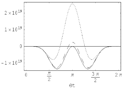
Figure 4: Marker of entanglement $\Upsilon^{(2)}$ between the Stokes sideband and the vibrational mode vs scaled time $t^{\prime}\equiv\Theta t$. The values of other parameters are: $r=1+2.5\times 10^{-7}$ and $\bar{n}=0$ (solid line), $\bar{n}=10^{-8}$ (dashed line), $\bar{n}=10^{-7}$ (dotted line).

Figure 5: Marker of entanglement $\Upsilon^{(2)}$ between the Stokes sideband and the vibrational mode vs scaled time $t^{\prime}\equiv\Theta t$ around $t^{\prime}=2\pi$. The values of other parameters are: $r=1+2.5\times 10^{-7}$ and $\bar{n}=10^{3}$. This shows that entanglement between the two modes persists even at high temperatures in this small time interval.

V Teleportation onto the state of the vibrational mode

We have seen that radiation pressure realizes an effective coupling between optical and acoustic modes. Since optical travelling beams are the typical playground for CV quantum information applications, this fact gives the possibility to involve also the vibrational modes of a mirror in the manipulation and storage of CV quantum information. The first experimental demonstration of a CV quantum information protocol has been the quantum teleportation of an unknown coherent state of an optical mode onto another optical mode illustrated in FUR98 and recently refined in BOW03 . We shall discuss how this CV quantum teleportation protocol can be adapted to the optomechanical system studied here in order to realize the teleportation of an unknown state of an optical field onto a vibrational mode of the mirror. This will allow us to present and discuss in more detail the optomechanical teleportation scheme of PRL03 . Quantum teleportation requires the use of shared entanglement between two distant stations, Alice and Bob, and of a classical channel for the transmission of the results of the Bell measurement from Alice to Bob BEN93 . The entanglement required is therefore that between the mirror vibrational mode and one optical mode. However, it is evident from the Hamiltonian of Eq. (14) and the bipartite entanglement analysis of the preceding Section that the relevant optical sideband mode is the Stokes mode. In fact, it interacts with the vibrational mode through the same parametric interaction generating two-mode squeezing which is at the basis of the optical version of the CV quantum teleportation protocol proposed in BRA98 and realized in FUR98 ; BOW03 . With this respect, the presence of the additional beam-splitter-like interaction with the antiStokes mode can only degrade the bipartite entanglement between the Stokes mode and the vibrational mode. The most straightforward way to implement teleportation in this optomechanical setting is just to apply the protocol of BRA98 and ignoring (i.e. tracing out) the disturbing antiStokes sideband mode. A schematic description of this solution is shown in Fig. 6. An unknown quantum state of a radiation field is prepared by a verifier (Victor) and sent to Alice, where it is mixed at a balanced beam splitter with the Stokes sideband mode with frequency $\omega_{0}-\Omega$. This latter mode is the only one reaching Alice station after reflection upon the mirror because the driving beam and the antiStokes mode are filtered out. The radiation pressure of the driving beam on the mirror establishes the required quantum channel, i.e. the shared entangled state between the mirror vibrational mode in Bob’s hand and the Stokes sideband at Alice station. It is evident from the analysis of Sections III and IV that this bipartite reduced state is still Gaussian, with CM

$$V_{1b}=\left(\begin{array}[]{cccc}{\cal A}+\frac{1}{2}&0&{\cal C}&0\\ 0&{\cal A}+\frac{1}{2}&0&-{\cal C}\\ {\cal C}&0&{\cal B}+\frac{1}{2}&0\\ 0&-{\cal C}&0&{\cal B}+\frac{1}{2}\end{array}\right)\,.$$ (37)

Then Alice carries out a balanced homodyne detection at each output port of the beam splitter, thereby measuring two commuting quadratures ${\hat{X}}_{+}=({\hat{X}}_{in}+{\hat{X}}_{1})/\sqrt{2}$ and ${\hat{P}}_{-}=({\hat{P}}_{in}-{\hat{P}}_{1})/\sqrt{2}$, with measurement results $X_{+}$ and $P_{-}$. The final step at the sending station is to transmit the classical information, corresponding to the result of the homodyne measurements she performed, to the receiving terminal. Upon receiving this information, Bob displaces his part of entangled state (the mirror acoustic mode) as follows: ${\hat{X}}_{b}\to{\hat{X}}_{b}+\sqrt{2}X_{+}$, ${\hat{P}}_{b}\to{\hat{P}}_{b}-\sqrt{2}P_{-}$. To actuate the phase-space displacement, Bob can use again the radiation pressure force. In fact, if the mirror is shined by a bichromatic intense laser field with frequencies $\varpi_{0}$ and $\varpi_{0}+\Omega$, it is easy to understand that, after averaging over the rapid oscillations, the radiation pressure force yields an effective interaction Hamiltonian $H_{act}\propto{\hat{b}}e^{-i\varphi}+{\hat{b}}^{{\dagger}}e^{i\varphi}$, where $\varphi$ is the relative phase between the two frequency components. Any phase space displacement of the mirror vibrational mode can be realized by adjusting this relative phase and the intensity of the laser beam.

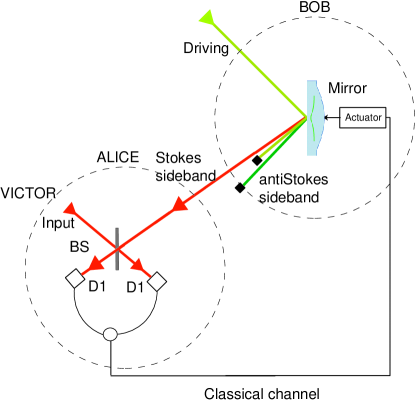
Figure 6: Scheme for the teleportation of an unknown quantum state of the optical mode provided by Victor to Alice onto the vibrational mode of the mirror. Only the Stokes sideband reaches Alice’s station and is mixed in the 50-50 beam splitter BS with the unknown input given by Victor. A Bell-like measurement $D1$ using homodyne detection is then performed on this combination and the result is fed-forward to Bob through the classical channel. Finally, he actuates the phase space displacement on the moving mirror.

In the case when Victor provides an input Gaussian state characterized by a $2\times 2$ CM $V^{in}$, the output state at Bob site is again Gaussian, with CM $V^{out}$. The input-output relation for these matrices can be found as follows. In terms of symmetrically ordered characteristic functions we have

$$\exp\left[-\sum_{i,j=1}^{2}u_{i}V^{out}_{ij}u_{j}\right]=\tilde{K}(u_{1},u_{2})\exp\left[-\sum_{i,j=1}^{2}u_{i}V^{in}_{ij}u_{j}\right]$$ (38)

where ${\bf u}$ is the variable vector of the characteristic functions and $\tilde{K}(u_{1},u_{2})$ can be written in terms of the symmetrically ordered characteristic function of the entangled state shared by Alice and Bob $\Phi_{sym}^{1b}(\mu,\nu)$ as

$$\tilde{K}(u_{1},u_{2}) = \int d^{2}kd^{2}\lambda d^{2}\mu d^{2}\nu\Phi_{sym}^{1b}(\mu,\nu)\exp\left\{-ik_{1}u_{1}-ik_{2}u_{2}+i\mu_{1}\lambda_{1}-i\mu_{2}\lambda_{2}+i\nu_{1}(k_{1}-\lambda_{1})+i\nu_{2}(k_{2}-\lambda_{2})\right\}$$ (39)

$$= \exp\left[-\sum_{i,j=1}^{4}w_{i}V^{1b}_{ij}w_{j}\right]\,,$$

where ${\bf w}=(u_{1},-u_{2},u_{1},u_{2})$. Then, it is easy to derive the input-output relation for these matrices (see also CHI02 )

$$V_{11}^{out} = V_{11}^{in}+\left(V^{1b}_{11}+2V^{1b}_{13}+V^{1b}_{33}\right)\,,$$ (40)

$$V_{12}^{out} = V_{12}^{in}+\left(V^{1b}_{14}-V^{1b}_{12}+V^{1b}_{34}-V^{1b}_{23}\right)\,,$$ (41)

$$V_{22}^{out} = V_{22}^{in}+\left(V^{1b}_{22}-2V^{1b}_{24}+V^{1b}_{44}\right)\,.$$ (42)

The fidelity $F$ of the described teleportation protocol, which is the probability to obtain the input state at Bob site, can be written, with the help of Eqs. (40)-(42) and (37), as

$$F=\{1+\left[1+{\cal A}+{\cal B}+2{\cal C}\right]\}^{-1}$$ (43)

where we have specialized to the case of an input coherent state. In such a case, the upper bound for the fidelity achievable with only classical means and no quantum resources is $F=1/2$ BRA99 . Fig. 7 shows the fidelity as a function of the interaction time $t^{\prime}$ only in the short time interval around $t^{\prime}=\Theta t=2\pi$ where it is appreciably different from zero. Different values of the initial mean thermal phonon number of the mirror acoustic mode $\overline{n}$ are considered ($\overline{n}=0$, 1, 10, $10^{3}$), and we have fixed again $r=1+2.5\times 10^{-7}$, as we have done in the preceding Section. The fidelity is appreciably different from zero only for interaction times $t^{\prime}$ slightly smaller than $2\pi$ and this time region corresponds just to the interaction time interval considered in Fig. 5 where the entanglement between the Stokes mode and the vibrational mode persists even at high mirror temperatures. The interesting result shown in Fig. 7 is that $F$ reaches a maximum value, $F_{max}\simeq 0.80$, which is well above the classical bound $F=0.5$ and that it is surprisingly independent of the initial temperature of the acoustic mode. This effect could be ascribed to quantum interference phenomena, and opens the way for the demonstration of quantum teleportation of states of mesoscopic massive systems composed of very many atoms. However the mirror temperature still has important disturbing effects, since by increasing $\overline{n}$, the useful time interval over which $F>1/2$ soon becomes extremely narrow, similarly to what happens to the visibility in the interference experiment proposed in marshall to detect the linear superposition of two macroscopically distinct states of a mirror. In the present proposal that means the need of designing precise driving laser pulses in order to have a well defined interaction time corresponding to the maximum of fidelity. This is however feasible using available pulse shaping techniques, since what is required here is simply a control of the laser pulse duration at the level of hundreds of nanoseconds.

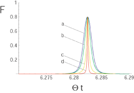
Figure 7: Fidelity $F$ vs the scaled time $t^{\prime}=\Theta t$ for the teleportation protocol of Fig. 6 in which the antiStokes mode is traced out. Curves a, b, c, d are for $\overline{n}=0$, 1, 10, $10^{3}$, respectively.

The results of Fig. 7 refer however to the straightforward procedure of ignoring the antiStokes mode. The fact that the teleportation process is not optimal, i.e. $F$ never reaches $1$, even asymptotically, can be ascribed to the fact that this “spectator” sideband mode carries away part of the quantum correlations which could be useful for teleportation. One could try therefore to adapt the original teleportation protocol of BRA98 to the present situation. A modified CV quantum teleportation protocol has been introduced in PRL03 : the antiStokes mode is not traced out but it is sent to Alice site as the Stokes mode and it is then subjected to a heterodyne measurement YUE80 (see Fig. (8)). Such a measurement serves the purpose of acquiring as much quantum information as possible about the tripartite entanglement between the two sideband modes and the vibrational mode and using it in a profitable way for teleportation. Performing an additional heterodyne measurement at Alice site certainly improves the protocol with respect to the scheme discussed above discarding the second sideband. Moreover it has the additional advantages of being easily implementable experimentally and of preserving the Gaussian nature of the entangled state of the Stokes and vibrational modes. On the other hand we have not proved that this is the best measurement Alice can perform on the $a_{2}$ mode to improve teleportation and therefore one cannot exclude that Alice, with appropriate measurements and local operations could get an even better result.

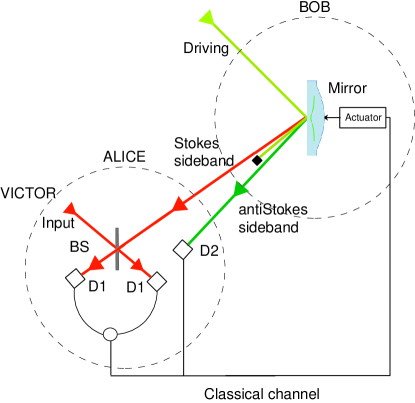
Figure 8: Improved scheme for the teleportation of an unknown quantum state of the optical mode provided by Victor to Alice onto the vibrational mode of the mirror. Both the Stokes and the antiStokes modes reach Alice’s station. The Stokes mode is mixed in the 50-50 beam splitter BS with the unknown input given by Victor as in the previous scheme of Fig. 6. The antiStokes mode is instead subject to a heterodyne measurement. The results of both the homodyne and heterodyne measurements are sent to Bob through the classical channel and he then uses this information to perform the appropriate phase-space displacement of the mirror.

When Alice performs the heterodyne measurement on the mode ${\hat{a}}_{2}$, the latter is projected onto a coherent state of complex amplitude $\alpha$ YUE80 . The Gaussian entangled state for the optical Stokes mode ${\hat{a}}_{1}$ and the vibrational mode $\hat{b}$, is now conditioned to this measurement result, which however explicitly appears only in first order moments, i.e. only the mean values of the quadratures. The CM of the resulting entangled state is instead independent of $\alpha$, and it is given by

$$V_{1b}^{het}=\left(\begin{array}[]{cccc}{\cal A}+\frac{1}{2}-\frac{{\cal F}^{2}}{{\cal E}+1}&0&{\cal C}+\frac{\cal FD}{{\cal E}+1}&0\\ 0&{\cal A}+\frac{1}{2}-\frac{{\cal F}^{2}}{{\cal E}+1}&0&-{\cal C}-\frac{\cal FD}{{\cal E}+1}\\ {\cal C}+\frac{\cal FD}{{\cal E}+1}&0&{\cal B}+\frac{1}{2}-\frac{{\cal D}^{2}}{{\cal E}+1}&0\\ 0&-{\cal C}-\frac{\cal FD}{{\cal E}+1}&0&{\cal B}+\frac{1}{2}-\frac{{\cal D}^{2}}{{\cal E}+1}\end{array}\right)\,.$$ (44)

Then the protocol proceeds in the same way as above. Alice carries out the homodyne measurement of the commuting quadratures ${\hat{X}}_{+}$ and ${\hat{P}}_{-}$, with measurement results $X_{+}$ and $P_{-}$ and then she sends the information corresponding to the results of both homodyne and heterodyne measurements to Bob, who now displaces his part of entangled state as follows: ${\hat{X}}_{b}\to{\hat{X}}_{b}+\sqrt{2}X_{+}+\sqrt{2}{\rm Re}\{\alpha\}({\cal F}-{\cal D})/({\cal E}+1)$, ${\hat{P}}_{b}\to{\hat{P}}_{b}-\sqrt{2}P_{-}+\sqrt{2}{\rm Im}\{\alpha\}({\cal F}+{\cal D})/({\cal E}+1)$. Notice that now Bob’s local operation depends on all Alice’s measurement results ($X_{+}$, $P_{-}$, $\alpha$). The final phase-space displacement of the mirror is realized in the same way as before. Also the input-output relation between the CM of the input state provided by Victor and the output state in Bob’s hands is the same as above, except that now the $4\times 4$ CM matrix of the shared entangled state $V^{1b}$ of Eq. (37) is replaced by the CM $V^{het}_{1b}$ of Eq. (44) in Eqs. (40)-(42).

The fidelity $F$ of this modified protocol, referred again to the case of an input coherent state, can be written as

$$F=\{1+\left[1+{\cal A}+{\cal B}+2{\cal C}-({\cal F}-{\cal D})^{2}/({\cal E}+1\right)]\}^{-1}\;,$$ (45)

and its behavior in the same interaction time interval around $t^{\prime}=2\pi$ and for the same four different values of $\bar{n}$ considered in Fig. 7 is shown in Fig. 9. Comparing Figs. 7 and 9, one sees that the improvement brought by this second protocol exploiting the additional heterodyne measurement is evident. Due to quantum interference, one has again a temperature-independent maximum fidelity, which is however larger than before, since it is $F_{max}\simeq 0.85$. The modified protocol is much more robust with respect to temperature and the time interval over which the fidelity is appreciably nonzero is now significantly larger, even though, at high temperatures, the time interval in which one has quantum teleportation, i.e. $F>1/2$, is still quite narrow and an accurate shaping of the driving laser pulse is still needed.

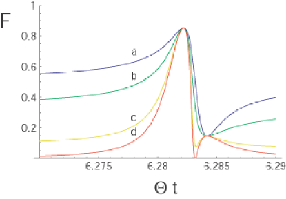
Figure 9: Fidelity $F$ vs the scaled time $t^{\prime}\equiv\Theta t$ for the improved teleportation protocol of Fig. 8 with the additional heterodyne measurement of the antiStokes mode. Curves a, b, c, d are for $\overline{n}=0$, 1, 10, $10^{3}$, respectively.

A quantitative comparison of the improvement brought by the additional heterodyne measurement on the antiStokes mode to the teleportation protocol can be made by evaluating the additional quantum information acquired by Alice with this measurement. This information can be evaluated in terms of the von Neumann entropies of the involved bipartite entangled states shared by Alice and Bob. In fact, we have seen that the effect of the heterodyne measurement on the antiStokes mode is to change the CM of the entangled state used as quantum channel for the teleportation. Therefore the quantum information gained by Alice with the heterodyne measurement is given by

$$\Delta S=S_{1b}-S_{1b}^{het}$$ (46)

where $S_{1b}=-$Tr$\left\{\rho_{1b}\log\rho_{1b}\right\}$ is the von Neumann entropy of the Gaussian entangled state of the Stokes mode and the vibrational mode when the antiStokes mode is traced out, with CM given by Eq. (37) and $S_{1b}^{het}=-$Tr$\left\{\rho_{1b}^{het}\log\rho_{1b}^{het}\right\}$ is the von Neumann entropy of the bipartite state conditioned to the result of the heterodyne measurement and with CM given by Eq. (44). These two entropies can be easily evaluated in terms of the CM of the two bipartite entangled states. In fact, using the results of serafini one has that the von Neumann entropy $S(V)$ of a bipartite Gaussian state with $4\times 4$ CM $V$, which is divided in $2\times 2$ blocks $A$, $B$ and $C$ as

$$V=\left(\begin{array}[]{cc}A&C\\ C^{T}&B\\ \end{array}\right)\,,$$ (47)

can be written as

$$S(V)=\sum_{i=+,-}\left[\left(n_{i}+\frac{1}{2}\right)\log\left(n_{i}+\frac{1}{2}\right)-\left(n_{i}-\frac{1}{2}\right)\log\left(n_{i}-\frac{1}{2}\right)\right]\;,$$ (48)

where

$$n_{\pm}=\sqrt{\frac{\Delta(V)\pm\sqrt{\Delta(V)^{2}-4{\rm Det}V}}{2}}$$ (49)

and

$$\Delta(V)={\rm Det}A+{\rm Det}B+2{\rm Det}C\;.$$ (50)

The behavior of the quantum information gained by Alice $\Delta S$ of Eq. (46) versus the interaction time $t^{\prime}$, in the same small time interval around $t^{\prime}=2\pi$ considered in Figs. 7 and 9 and for different values of the initial mean vibrational number $\bar{n}$ is plotted in Fig. 10. We see that the information acquired through the heterodyne measurement increases for larger temperatures, i.e., the modified protocol becomes particularly useful at higher temperatures. This is in agreement with the fact that the modified protocol with the additional heterodyne measurement is much more robust with respect to temperature than the one based on tracing out the antiStokes mode, as showed by Figs. 7 and 9. In Fig. 10 we see also that the quantum information gain $\Delta S$ drops to zero at all temperatures at exactly $t^{\prime}=2\pi$, because at this interaction time the bipartite reduced state of the Stokes and the vibrational modes becomes the chosen factorized initial state of Eq. (24), i.e. the product of a thermal equilibrium state for the vibrational mode and the vacuum state for the optical sideband, either with or without the additional heterodyne measurement.

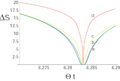
Figure 10: Information gain $\Delta S$ brought by the heterodyne measurement vs the scaled time $t^{\prime}\equiv\Theta t$ in the same small time interval around $t=2\pi$ considered in Figs. 7 and 9 for different values of the mirror mean vibrational number $\bar{n}$. Curves a, b, c, d are for $\overline{n}=0$, 1, 10, $10^{3}$, respectively.

VI Discussion of the results and concluding remarks

We have seen that the optomechanical entanglement between the Stokes sideband mode and a vibrational mode of a mirror can be profitably used for the teleportation of an arbitrary state of a radiation mode onto the quantum state of the vibrational mode. This would imply the remarkable capability of manipulating CV quantum information with objects with a macroscopic number of atoms. For example, the possibility to “write” the state of an optical beam onto an acoustic mode implies the possibility to perform a very fast ground state cooling of the mirror vibrational mode. In fact, in this case, cooling is nothing but the teleportation of the optical vacuum state provided by Victor onto the state of the mirror vibrational mode. This “telecooling” is very fast and it exploits the optomechanical entanglement created by radiation pressure. As a matter of fact, the effective number of thermal excitations of the vibrational mode soon after the two homodyne and the heterodyne measurements at Alice station (in the improved protocol of Fig. 8) becomes $\overline{n}_{eff}=1+{\cal A}+{\cal B}+2{\cal C}-({\cal F}-{\cal D})^{2}/({\cal E}+1)$. It reduces to $\overline{n}+1$ in absence of entanglement, where $1$ represents the noise introduced by the protocol. Instead, the optomechanical interaction for a proper time permits to achieve $\overline{n}_{eff}=0.17$ at once, at the moment of Alice’s measurement, thanks to the nonlocal quantum correlations between the mirror mode and the light mode at Alice’s station.

A remarkable aspect of the present scheme is the robustness of the tripartite entanglement between the two motional sidebands and the vibrational mode with respect to the mirror temperature. In fact, the three modes are almost always entangled, at any temperature, and this holds provided that the interaction time, i.e. the duration of the driving laser pulse is much smaller than the mirror mode decay rate. In this case, the coupling of the mirror with its environment can be neglected and the dynamics of the three-mode system is purely Hamiltonian, so that quantum coherence effects can still survive even for a highly mixed mirror initial state. On the other hand, thermal noise has still important effects: i) the interaction time window in which the protocol is efficient becomes narrower and narrower for increasing temperature (see the previous Section); ii) the time interval within which the classical communication from Alice to Bob, and the phase space displacement by Bob have to be made, becomes shorter and shorter with increasing temperature, because the vibrational state projected by Alice’s Bell measurement heats up in a time of the order of $(\gamma_{m}\overline{n})^{-1}$, where $\gamma_{m}$ is the mechanical damping constant. Therefore, despite this robustness, in practice, any experimental implementation will still need an acoustic mode cooled at low temperatures (see however Refs. COH99 ; VIT02 for effective cooling mechanism of acoustic modes).

The effects of mechanical damping can be neglected during the back-scattering process stimulated by the intense laser beam when the parameter $\Theta$, whose inverse fixes the dynamical timescale of the process, is much larger than the decay rate $\gamma_{m}$. Mechanical damping rates of about $\gamma_{m}\simeq 1$ Hz are available TIT99 , and therefore choosing $\chi\simeq\theta\simeq 5\times 10^{5}$ Hz, and $r-1=2.5\times 10^{-7}$ one has $\Theta=\sqrt{\theta^{2}-\chi^{2}}\simeq 10^{3}$ Hz, which means using a highly monochromatic laser pulse with a duration of milliseconds. Such values for the coupling constants $\chi$ and $\theta$ can be obtained for example choosing ${\wp}=10$W, $\omega_{0}\sim 2\times 10^{15}$ Hz, $\Omega\sim 5\times 10^{8}$ Hz, $\Delta\nu_{det}\sim 10^{7}$ Hz, $\Delta\nu_{mode}\sim t^{-1}\sim 10^{3}$ Hz, and $M\sim 10^{-10}$ Kg. These parameters are partly different from those of already performed optomechanical experiments TIT99 ; COH99 . However, using a thinner silica crystal and considering higher frequency modes, the parameters we choose could be obtained. On the other hand performing a quantum teleportation experiment on a collective mode of a mirror involving about $10^{15}$ atoms is not trivial at all and the technical difficulties in the realization of this experiment are not surprising. Such low effective masses of the involved vibrational mode could be achieved for example in micro-opto-electro-mechanical systems (MOEMS), which possess vibrational modes with a very high oscillation frequency $\Omega$ ROU03 .

There are also other sources of imperfection besides the thermal noise acting on the mechanical resonator. Other fundamental noise sources are the shot noise and the radiation pressure noise. Shot noise affects the detection of the sideband modes but its effect is already taken into account by our treatment (it is responsible for the $1/2$ terms in the diagonal entries of the correlation matrix of Eqs. (37) and (44)). The radiation pressure noise due to the intensity fluctuations of the incident laser beam yields fluctuations of the optomechanical coupling. However, the chosen parameter values give $\Delta\wp/\wp=\Delta(\Theta t)/2\Theta t\simeq 10^{-8}$, which is negligibly small with respect to the width of the window where the fidelity attains its maximum (see Figs. 7 and 9).

Finally, one has also to verify that the teleportation has been effectively realized, that is, that the state provided by Victor has been transferred to the mirror vibrational mode. This implies measuring the final state of the acoustic mode, and this can be done by considering a second, intense “reading” laser pulse, and exploit again the optomechanical interaction given by Eq. (14), where now $a_{1}$ and $a_{2}$ are output meter modes. It is in fact possible to perform a heterodyne measurement of an appropriate combination of the two back-scattered modes, ${\hat{Z}}={\hat{a}}_{1}-{\hat{a}}_{2}^{{\dagger}}$, if the driving laser beam at frequency $\omega_{0}$ is used as local oscillator and the resulting photocurrent is mixed with a signal oscillating at the frequency $\Omega$. The behaviour of $Z(t)$ as a function of the time duration of the second “measuring” driving beam can be derived from Eqs. (17)-(19), that is

$${\hat{Z}}(t)\equiv{\hat{a}}_{1}(t)-{\hat{a}}_{2}^{{\dagger}}(t) = \frac{1}{\Theta}\left[\chi+\theta\right]\sin(\Theta t){\hat{b}}^{{\dagger}}(0)$$ (51)

$$+ \frac{1}{\Theta^{2}}\left[\theta^{2}-\chi^{2}\cos(\Theta t)-\chi\theta+\chi\theta\cos(\Theta t)\right]{\hat{a}}_{1}(0)$$

$$- \frac{1}{\Theta^{2}}\left[\chi\theta+\chi\theta\cos(\Theta t)-\chi^{2}-\theta^{2}\cos(\Theta t)\right]{\hat{a}}_{2}^{{\dagger}}(0)\,.$$

It is easy to see that for $\cos(\Theta t)=0$ and $\Theta(\theta+\chi)\gg\theta(\theta-\chi)$ the measured quantity practically coincides with the mode oscillation operator $b^{{\dagger}}(0)$, thus revealing information on the state of the mechanical oscillator.

To summarize, we have seen that the radiation pressure of an intense and quasi-monochromatic laser pulse incident on a perfectly reflecting mirror is able to entangle a mirror vibrational mode with the two first optical sidebands of the driving mode. The three-mode CV system shows almost always fully tripartite entanglement for any value of the mirror temperature, provided that the coupling of the mirror mode with its environment can be neglected during the optomechanical interaction. In particular, the bipartite entanglement between the Stokes sideband mode and the mirror vibrational mode can be used to implement the teleportation of an unknown quantum state of a radiation field onto a macroscopic, collective vibrational degree of freedom of a massive mirror.

The present result could be challenging tested with present technology, and opens new perspectives towards the use of quantum mechanics in macroscopic world.

References

- (1) C. H. Bennett, et al., Phys. Rev. Lett. 70, 1895 (1993).
- (2) C. H. Bennett and S. Wiesner, Phys. Rev. Lett. 69, 2881 (1992).
- (3) A.K. Ekert, Phys. Rev. Lett. 67, 661 (1991).
- (4) L. Vaidman, Phys. Rev. A 49, 1473 (1994).
- (5) S. L. Braunstein and H. J. Kimble, Phys. Rev. Lett. 80, 869 (1998).
- (6) A. Furusawa, et al. Science 282, 706 (1998).
- (7) W. P. Bowen, N. Treps, B. C. Buchler, R. Schnabel, T. C. Ralph, H.-A. Bachor, T. Symul, and P. K. Lam Phys. Rev. A 67, 032302 (2003); T. C. Zhang, K. W. Goh, C. W. Chou, P. Lodahl, and H. J. Kimble Phys. Rev. A 67, 033802 (2003).
- (8) M. Ban, J. Opt. B1, L9 (1999); S.L. Braunstein and H.J. Kimble, Phys. Rev. A 61, 042302 (2000); X. Li et al., Phys. Rev. Lett. 88, 047904 (2002).
- (9) T.C. Ralph, Phys. Rev. A 61, 010303(R) (2000); M. Hillery, Phys. Rev. A 61, 022309 (2000); S.F. Pereira, Z.Y. Ou and H.J. Kimble, Phys. Rev. A 62, 042311 (2000); M.D. Reid, Phys. Rev. A 62, 062308 (2000); F. Grosshans and P. Grangier, Phys. Rev. Lett. 88, 057902 (2002).
- (10) F. Grosshans et al., Nature 421, 238 (2003).
- (11) S. Lloyd and S.L. Braunstein, Phys. Rev. Lett. 82, 1784 (1999).
- (12) A. Einstein, B. Podolsky and N. Rosen, Phys Rev. 47, 777 (1935).
- (13) D. F. Walls and G. J. Milburn, Quantum Optics, (Springer, Berlin, 1994).
- (14) A.E. Kozhekin, K. Molmer and E. Polzik, Phys. Rev. A 62, 033809 (2000); L.-M Duan, J. I. Cirac, P. Zoller and E. Polzik, Phys. Rev. Lett. 85, 5643 (2000).
- (15) B. Julsgaard, A. Kozhekin and E. S. Polzik, Nature (London) 413, 400 (2001).
- (16) A.S. Parkins and H.J. Kimble, Phys. Rev. A 61, 052104 (2000); A.S. Parkins and E. Larsabal, Phys. Rev. A 63, 012304 (2001).
- (17) S. Mancini, V. Giovannetti, D. Vitali and P. Tombesi, Phys. Rev. Lett. 88, 120401 (2002); Eur. J. Phys. D, 22, 417 (2003).
- (18) S. Mancini, D. Vitali, and P. Tombesi, Phys. Rev. Lett. 90, 137901 (2003).
- (19) G.R. Gunthorlein et al., Nature 414, 49 (2001); A.B. Mundt et al., Phys. Rev. Lett. 89, 103001 (2002); J. McKeever, J. R. Buck, A. D. Boozer, A. Kuzmich, H.-C. N gerl, D. M. Stamper-Kurn, and H. J. Kimble Phys. Rev. Lett. 90, 133602 (2003) .
- (20) C. Fabre, M. Pinard, S. Bourzeix, A. Heidmann, E. Giacobino and S. Reynaud, Phys. Rev. A 49, 1337 (1994).
- (21) S. Mancini and P. Tombesi, Phys. Rev. A 49, 4055 (1994).
- (22) S. Mancini, V. I. Man’ko and P. Tombesi, Phys. Rev. A 55, 3042 (1997); S. Bose, K. Jacobs and P. L. Knight, Phys. Rev. A 56, 4175 (1997).
- (23) W. Marshall, C. Simon, R. Penrose, D. Bouwmeester, Phys. Rev. Lett. 91, 130401 (2003).
- (24) A. Dorsel, J.D. McCullen, P. Meystre, E. Vignes, and H. Walther, Phys. Rev. Lett. 51, 1550 (1983); A. Gozzini, F. Maccarone, F. Mango, I. Longo, and S. Barbarino, J. Opt. Soc. Am. B 2, 1841 (1985).
- (25) V. Giovannetti, S. Mancini and P. Tombesi, Europhys. Lett. 54, 559 (2001).
- (26) S. Mancini and A. Gatti, J. Opt. B: Quantum and Semiclass. Opt. 3, S66 (2001).
- (27) S. Giannini, S. Mancini and P. Tombesi, Quantum Inf. Comput. 3 265 (2003).
- (28) M. Pinard, et al., Eur. Phys. J. D 7, 107 (1999).
- (29) P. Samphire, R. Loudon, and M. Babiker, Phys. Rev. A 51, 2726 (1995).
- (30) J. Perina, Quantum Statistics of Linear and Nonlinear Optical Phenomena, (Reidel, Dordrecht, 1984).
- (31) R. A. Andrews, H. Rabin, and C.L. Tang, Phys. Rev. Lett. 25, 605 (1970).
- (32) M. E. Smithers, and E. Y. C. Lu, Phys. Rev. A 10, 1874 (1974).
- (33) A. Ferraro, M. G. A. Paris, A. Allevi, W. Andreoni, M. Bondani, and E. Puddu, e-print quant-ph/0306109.
- (34) E. I. Mason, N. C. Wong, Opt. Lett. 23, 1733 (1998); H. H. Adamyan, G. Yu. Kryuchkyan, e-print quant-ph/0309203.
- (35) M. G. A. Paris, M. Cola, N. Piovella and R. Bonifacio, e-print quant-ph/0302155.
- (36) I. Tittonen, et al., Phys. Rev. A 59, 1038 (1999).
- (37) W. Dür, J. I. Cirac, and R. Tarrach, Phys. Rev. Lett. 83, 3562 (1999); W. Dür and J. I. Cirac, Phys. Rev. A 61, 042314 (2000).
- (38) S. Pirandola, S. Mancini, D. Vitali, and P. Tombesi, J. Opt. B: Quantum Semiclass. Opt. 5, S523-S529 (2003).
- (39) G. Giedke, B. Kraus, M. Lewenstein, and J. I. Cirac, Phys. Rev. A 64, 052303 (2001).
- (40) R. F. Werner and M. M. Wolf, Phys. Rev. Lett. 86, 3658 (2001).
- (41) Actually we have only considered values of very close to , because they are the only ones which are physically significant.
- (42) G. Vidal and R. F. Werner, Phys. Rev. A 65, 032314 (2002).
- (43) R. Simon, Phys. Rev. Lett. 84, 2726 (2000)
- (44) M. S. Kim, W. Son, V. Bužek, and P. L. Knight, Phys. Rev. A 65, 032323 (2002).
- (45) A. V. Chizhov, L. Knöll and D. G. Welsch, Phys. Rev. A 65, 022310 (2002).
- (46) S. L. Braunstein, C. A. Fuchs, H. J. Kimble and P. van Loock, Phys. Rev. A 64, 022321 (2001).
- (47) H. P. Yuen and J. H. Shapiro, IEEE Trans. Info. Theory IT-26, 78 (1980).
- (48) A. Serafini, F. Illuminati, and S. De Siena, e-print quant-ph/0307073.
- (49) P. F. Cohadon, A. Heidmann and M. Pinard, Phys. Rev. Lett. 83, 3174 (1999).
- (50) D. Vitali, S. Mancini, L. Ribichini and P. Tombesi, Phys. Rev. A 65, 063803 (2002).
- (51) X. M. H. Huang, C. A. Zorman, M. Mehregany, and M. L. Roukes, Nature (London) 421, 496 (2003).