Two interacting hard disks within a circular cavity:
towards a quantal equation of states

Abstract

We investigate a circular cavity billiard within which a pair of identical hard disks of smaller but finite size is confined. Each disk shows a free motion except when bouncing elastically with its partner and with the boundary wall. Despite its circular symmetry, this system is nonintegrable and almost chaotic because of the (short-range) interaction between the disks. We quantize the system by incorporating the excluded volume effect for the wavefunction. Eigenvalues and eigenfunctions are obtained by tuning the relative size between the disks and the billiard. We define the volume $V$ of the cavity and the pressure $P$, i.e., the derivative of each eigenvalue with respect to $V$. Reflecting the fact that the energy spectra of eigenvalues versus the disk size show a multitude of level repulsions, $P-V$ characteristics shows the anomalous fluctuations accompanied by many van der Waals-like peaks in each of individual excited eigenstates taken as a quasi-equilibrium. For each eigenstate, we calculate the expectation values of the square distance between two disks, and point out their relationship with the pressure fluctuations.

I Introduction

The study of classical and quantum billiards has a long history Krylov79 ; Arnold68 ; Bunimovich80 ; Gaspard98 ; Gaspard89 . From a viewpoint of classical dynamics, cavity billiards are classified into two categories according to their integrability or nonintegrability Lichtenberg83 . The stadium is a prototype of the nonintegrable and chaotic billiards, whereas highly-symmetric billiards like circle, triangle and square are integrable and regular. The quantum-mechanical feature of these billiards such as level statistics is nowadays well known Giannoni89 ; Stockmann99 .

Most of the studies so far, however, are limited to the systems of a single point particle or a single disk confined in billiards. There exists little work on the billiards which contain a finite number of mutually-interacting particles Awazu01 ; Ahn99 ; Papenbrock00 . The interaction between particles will make the system nonintegrable and chaotic even if the confining cavity is highly symmetric. On the other hand, recent development in hightechnology has fabricated quantum dots and optically-trapped atoms where a finite number of interacting particles are trapped in a small area. Quantum mechanics of these systems constitutes a topical subject Tarucha96 ; Kouwenhoven97 .

Considering the above circumstances, we want to understand what kind of novel phenomena should occur in the cavity billiards where interacting small particles are embedded. In this paper, we consider a pair of identical hard disks of finite size accommodated in a circular cavity. Each disk is assumed to bounce elastically with its partner and with the boundary wall, but otherwise showing a ballistic motion. Although the system is circularly symmetric, it is nonintegrable and chaotic thanks to the (short-range) interaction between the disks, as proved in the following analysis of classical dynamics.

The tunable control parameter of the system is an aspect ratio of the radii between each disk and the circular cavity. When the aspect ratio is varied, how do the quantal eigenvalues and eigenfunctions behave? A multitude of level repulsions and level-spacing distributions like Wigner distribution will be shown to appear. Recalling the similarity between the present system and a nonideal gas confined within a container, the most important feature of this system would be a quantal equation of states, i.e., the volume $V$ dependence of the pressure $P$ at the cavity wall. Under a fixed radius of each disk, tuning of the aspect ratio corresponds to contraction or expansion of the volume $V$ of the circular cavity. The pressure $P$ at the wall boundary is obtained from the derivative of parameter-dependent eigenvalues with respect to $V$. In the classical nonideal gas theory, $P$ does not decrease monotonically as $V$ is increased, and is accompanied by the van der Waals peak. This peak appears due to the competition between the finite size of each molecule and the attractive interaction between molecules. In the present system, we find the competition between the finite size of each disk and the quantum-mechanical correlation due to symmetrization of two-particle wavefunctions. Therefore $P-V$ characteristics in the present system is expected to exhibit novel fluctuations unseen in ordinary quantum billiards that contain only a single particle or disk. This is an advantage of the interacting disk systems over the ordinary quantum billiards. By using two-particle wave functions, we shall evaluate expectation values for the distance between disks, which will elucidate a physical mechanism for fluctuations in the quantal equation of states.

The organization of the paper is as follows: In Section II, we shall introduce a model system and analyze the underlying classical dynamics. We shall compute the maximum Lyapunov exponent with use of a modern technique by Gaspard and Beijeren Gaspard02 . In Section III we define the two-particle basis wavefunctions appropriate to quantize this complicated system and describe some technical details to obtain a standard form of the eigenvalue equation. The result for eigenvalues is given for various aspect ratios in Section IV. Here we shall also analyze $P-V$ characteristics, which will be the central theme of our study. Section V is devoted to investigation of expectation values for the distance between disks, where the single-particle density and two-particle correlation functions are exploited. The final Section is concerned with summary and discussions.

II Model system and classical dynamics

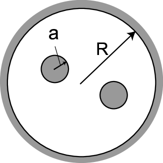
Figure 1: Model system.

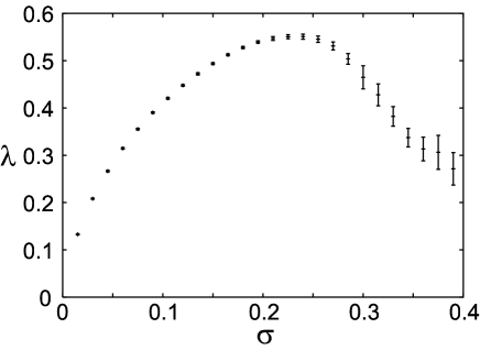
Figure 2: The ratio $\sigma=a/R$ vs. the maximum Lyapunov exponent $\lambda$ calculated by the numerical simulation. The total $L_{z}$ is taken as zero. The error bar means the standard deviation of obtained $\lambda$’s.

Figure 1 illustrates our model system consisting of two identical hard disks moving within a circle billiard. Each disk shows a ballistic motion except when bouncing with its partner and with the billiard boundary. Let $R$ and $a(<R/2)$ be the radii for the circle billiard and each disk, respectively. Here the internal self-rotation (spinning motion) of each disk are ignored. The single-disk motion in the circle billiard is integrable since the number of degrees of freedom (two) accords with that of constants of motion, i.e., energy and angular momentum. However, the two-disk system proposed here has the degree of freedom (four) which is larger than the number of constants of motion, i.e., the total energy, angular momentum. Therefore the system becomes nonintegrable, and may be chaotic.

The chaotic dynamics is characterized by the positive maximum Lyapunov exponent $\lambda$. This can be obtained by numerical simulation for a given initial condition by using linearized equations for deviations of an orbit. Although the degrees of freedom is four in the present system, the calculation of $\lambda$ is greatly simplified because of the nature of billiard motion Gaspard95 ; Gaspard02 . For the evaluation of $\lambda$, each orbit is calculated over $N_{\rm col}=10^{6}$ collisions. Generally, $\lambda$ depends on the initial conditions. We randomly choose $N_{\rm init}=10^{5}$ initial conditions satisfying $L_{z}=0$. The average and standard deviation of obtained $\lambda$’s are shown in Fig. 2. For $0<\sigma=a/R<0.4$, the positive maximum Lyapunov exponent can be observed. The standard deviation systematically decreases below $\sigma\sim 0.25$ as $N_{\rm col}$ increases. The convergence, however, is not observed above $\sigma\sim 0.25$ as shown by large standard deviations; This indicates that the ergodicity is not guaranteed in this region.

Through the numerical simulation, we found that a small amount of initial conditions leads to $\lambda=0$ indicating the existence of tori in the phase space in the full region of $\sigma$. The ratio of tori to the whole phase space is, however, extremely small, and is estimated typically as smaller than of $10^{-3}$. Although the present system should be said exactly to be a mixed system, the chaotic sea occupies almost whole part of the phase space, and one can proceed to investigate a quantum analogue of chaos in this system.

III Methodology of quantization

To make variables dimensionless, we choose the scaling for coordinates and energy as

$${\bf r}^{\prime}=\frac{{\bf r}}{R-a}, a^{\prime}=\frac{a}{R-a},$$

$$R^{\prime}=\frac{R}{R-a}, E^{\prime}=\frac{E}{\frac{{\hbar}^{2}}{2m(R-a)^{2}}}.$$ (1)

Note that by this scaling the ratio $\sigma=a/R=a^{\prime}/R^{\prime}$ is not changed. By the above scaling, the admissible range for $r^{\prime}=|{\bf r}^{\prime}|$ becomes $0\leq r^{\prime}\leq 1$. Hamiltonian is then given in a dimensionless form as

$$H=-\sum_{i=1,2}\left(\frac{\partial^{2}}{\partial r^{\prime 2}_{i}}+\frac{1}{r^{\prime}_{i}}\frac{\partial}{\partial r^{\prime}_{i}}+\frac{1}{r^{\prime 2}_{i}}\frac{\partial^{2}}{\partial\theta^{\prime 2}_{i}}\right)+\sum_{i=1,2}U({\bf r}^{\prime}_{i})+V(|{\bf r}^{\prime}_{1}-{\bf r}^{\prime}_{2}|),$$ (2)

where

$$U({\bf r}^{\prime}_{i})=\left\{\begin{array}[]{cl}\infty&(|{\bf r}^{\prime}_{i}|\geq 1)\\ 0&(|{\bf r}^{\prime}_{i}|<1)\end{array}\right.,$$ (3)

and

$$V(\xi)=\left\{\begin{array}[]{cl}0&(\xi\geq 2a^{\prime})\\ \infty&(\xi<2a^{\prime})\end{array}\right..$$ (4)

The second and third terms in (2) represent confining potential by the hard wall of the circle billiard and inter-disk interaction due to their hard cores, respectively. In the case of a single disk inside the circle billiard, the appropriate wavefunction satisfying the boundary condition is given by Bessel function of integer order for the radial part multiplied by the angular function as

$$J_{k}(\lambda_{kn}r^{\prime})e^{ik\theta^{\prime}},$$ (5)

where $k$ and $n$ are integers and $J_{k}(\lambda_{kn}r^{\prime})$ vanishes at $r^{\prime}=1$, namely at the boundary wall. By choosing the wavefunction (5) for each of the disks, Dirichlet boundary condition represented by the potential $U({\bf r}^{\prime}_{i})$ is automatically satisfied. On the other hand, the basis functions for the two-disk system are given by a product of (5) and take

$$\Phi_{\alpha}=J_{k_{1}}(\lambda_{k_{1}n_{1}}r^{\prime}_{1})J_{k_{2}}(\lambda_{k_{2}n_{2}}r^{\prime}_{2})e^{ik_{1}\theta^{\prime}_{1}}e^{ik_{2}\theta^{\prime}_{2}}f(X),$$ (6)

which are as yet not orthonormal. The multiplicative factor $f(X)$, which represents the excluded volume effect caused by the hard cores of the disks, is defined by

$$f(X)=\left\{\begin{array}[]{cl}\ 1-e^{-\beta X}&(X>0)\\ 0&(X\leq 0)\end{array}\right..$$ (9)

Here $X\equiv r^{\prime 2}_{1}+r^{\prime 2}_{2}-2r^{\prime}_{1}r^{\prime}_{2}\cos\phi-l_{0}^{2}$ with $\phi=\theta^{\prime}_{2}-\theta^{\prime}_{1}$ and $l_{0}=2a^{\prime}$. $X$ stands for a void between two hard disks, $\phi$ is a relative angle, and $l_{0}$ is the admissible minimum distance between the centers of two hard disks, at which they touch each other. $\beta$ is arbitrary positive real number, and may be called as the fictitious inverse temperature. We will discuss about $\beta$ at the end of this Section. $\Phi_{\alpha}$ vanishes at $X=0$, satisfying another boundary condition that the wavefunction for two disks should vanish when they touch each other. In other words, the inclusion of the factor $f(X)$ is approximately identical to incorporating the effect of the short-range repulsive interaction $V(|{\bf r}^{\prime}_{1}-{\bf r}^{\prime}_{2}|)$ in (2). Finally we symmetrize the wavefunction noting the indistinguishability of two disks. We here choose a symmetrized wave function by assuming the invariance of wavefunctions against the exchange of the disk coordinates. This choice is appropriate when the disks are Boson or Fermion forming a spin-singlet state. Therefore we use the basis function defined by

$$\Psi_{\alpha}=(\Phi_{\alpha}(1,2)+\Phi_{\alpha}(2,1))/\sqrt{2}.$$ (10)

With use of (10) we shall proceed to construct the energy matrices. First, by operating the Hamiltonian (2) on (10), we find

$$H\Psi_{\alpha} = ({\lambda_{k_{1}n_{1}}}^{2}+{\lambda_{k_{2}n_{2}}}^{2})\Psi_{\alpha}$$ (11)

$$+ \frac{1}{\sqrt{2}}\Biggl{[}\,\biggl{\{}-8\beta J_{k_{1}}J_{k_{2}}e^{ik_{1}\theta^{\prime}_{1}}e^{ik_{2}\theta^{\prime}_{2}}e^{-\beta X}(1-\beta({r^{\prime}_{1}}^{2}+{r^{\prime}_{2}}^{2}-2r^{\prime}_{1}r^{\prime}_{2}\cos\phi))\biggr{.}\Biggr{.}$$

$$-4\beta e^{ik_{1}\theta^{\prime}_{1}}e^{ik_{2}\theta^{\prime}_{2}}e^{-\beta X}\left(J_{k_{2}}\frac{\partial J_{k_{1}}}{\partial r^{\prime}_{1}}(r^{\prime}_{1}-r^{\prime}_{2}\cos\phi)+J_{k_{1}}\frac{\partial J_{k_{2}}}{\partial r^{\prime}_{2}}(r^{\prime}_{2}-r^{\prime}_{1}\cos\phi)\right)$$

$$\biggl{.}+4i\beta J_{k_{1}}J_{k_{2}}e^{ik_{1}\theta^{\prime}_{1}}e^{ik_{2}\theta^{\prime}_{2}}e^{-\beta X}\sin\phi\left(\frac{r^{\prime}_{2}}{r^{\prime}_{1}}k_{1}-\frac{r^{\prime}_{1}}{r^{\prime}_{2}}k_{2}\right)\biggr{\}}$$

$$+\Biggl{.}\biggl{\{}1\leftrightarrow 2\ \biggr{\}}\Biggr{]}.$$

Second, multiplying (11) by ”$bra$” that corresponds to the complex conjugate of (10), we integrate each term over coordinates. The integration about angles $\theta^{\prime}_{1}$, $\theta^{\prime}_{2}$ can be performed analytically. But we have to carry out the numerical integration about the radial coordinates $r^{\prime}_{1}$, $r^{\prime}_{2}$. Third, noting that the total angular momentum $L_{z}$ is a good quantum number, we diagonalize the energy matrices for each of the fixed value $L_{z}$. That is $k_{1}+k_{2}=k_{1}^{\prime}+k_{2}^{\prime}=L_{z}$ with $L_{z}=0,\pm 1,\pm 2$, and so on.

Finally, before proceeding to diagonalization of each energy matrix, it must be regularized because we are using non-orthogonal basis functions. This is performed as follows: In the eigenvalue problem $H\Psi=E\Psi$ under consideration, we substitute the expansion $\Psi=\sum_{\alpha}C_{\alpha}\Psi_{\alpha}$ with $\Psi_{\alpha}$ the non-orthogonal basis functions. Then one reaches

$$\sum_{\alpha}H_{\alpha^{\prime}\alpha}C_{\alpha}=\sum_{\alpha}EN_{\alpha^{\prime}\alpha}C_{\alpha},$$ (12)

with $H_{\alpha^{\prime}\alpha}=\langle\Psi_{\alpha^{\prime}}|H|\Psi_{\alpha}\rangle$ and $\langle\Psi_{\alpha^{\prime}}|\Psi_{\alpha}\rangle=N_{\alpha^{\prime}\alpha}\neq\delta_{\alpha^{\prime}\alpha}$.

With use of the diagonalized norm-kernel $N_{d}$ obtained by

$$U^{-1}NU\rightarrow N_{d},$$ (13)

we introduce the regularized energy matrix

$$\tilde{H}=N_{d}^{-1/2}U^{-1}HUN_{d}^{-1/2}.$$ (14)

As a consequence, we arrive at a standard form of the eigenvalue equation

$$\tilde{H}{\bf g}=E{\bf g},$$ (15)

where ${\bf g}=N_{d}^{1/2}U^{-1}{\bf C}$. This equation will be solved in the next Section.

Before closing this Section, we should comment on the fictitious inverse temperature $\beta$ involved in the excluded-volume effect factor $f(X)$ in (9). We find the calculated eigenvalues are stable against variation of $\beta$ so long as it falls in $0.5<\beta<3.0$ so that we shall fix to $\beta=1.5$.

IV Energy spectra and pressure

IV.1 Eigenvalues and level-spacing distribution

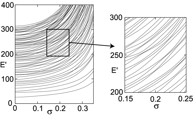
Figure 3: Energy levels versus ratio of radii ($\sigma$) between each disk and a circle billiard in the manifold $L_{z}=1$. Inset is a partial magnification.

We prescribe $\sigma=a/R$ with $0\leq\sigma\leq 0.5$ as a tunable parameter controlling the size of the disk. Under a fixed angular momentum $L_{z}$, we diagonalize the energy matrix in $10^{3}\times 10^{3}$ dimensions by varying $\sigma$. The lower half of $10^{3}$ eigenvalues, which have a precision of 4 digits, is used for our study below. In the manifold $L_{z}=1$, the energy spectrum against $\sigma$ is given in Fig. 3. The upward shifts of energies as a whole with increasing $\sigma$ reflect the confining of disks in a rapidly-decreasing effective area inside the wall boundary. This spectrum together with its partial magnification shows a multitude of avoided level crossings (level repulsions). Except for the lower energy region, the avoided crossings are widely seen in the full range of $0<\sigma<0.5$.

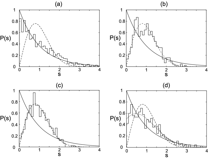
Figure 4: Histogram of level-space distribution: (a)Noninteracting disks with $\sigma=0.2$ and $L_{z}=1$; (b)Interacting disks with $\sigma=+0$ and $L_{z}=1$; (c)Interacting disks with $\sigma=0.2$ and $L_{z}=1$; (d)Interacting disks with $\sigma=0.2$ and $L_{z}=0$. The solid, dashed and dotted curves show the Poisson distribution, Wigner distribution and the mixture of two independent Wigner distributions, respectively.

We proceed to investigate the level-spacing distributions, where the usual unfolding procedure is performed Haake00 ; Mehta91 . Figures 4 (a)-(c) are the level-spacing distributions $P(s)$ for typical values of $\sigma$ with $L_{z}=1$, obtained from intermediate $450$ levels by suppressing both the lowest $50$ levels and the upper half of $10^{3}$ levels. Figure 4 (a) is the result for the noninteracting two-disk system within the circle billiard, which approximately provides Poisson distribution $P(s)=\exp(-s)$. Small deviation from the Poisson distribution is however observed; We infer that this deviation comes from the particular properties of the zero points of the Bessel function which tends to be periodic in the asymptotic limit. In the case of interacting disks under consideration, the Wigner distribution $P(s)=\frac{\pi}{2}\exp(-\pi s^{2})$ can be seen in the full range of $0\leq\sigma\leq 0.5$. This distribution is known as a quantal signature of chaos. It is interesting that Wigner distribution is obtained even in the point-disk limit, $\sigma=+0$. This is due to the fact that, in this limit, the present system has a short-range interaction of delta-function type, and is distinct from a noninteracting two-disk system. The stability of level statistics against the variation of $\sigma$ is very convenient in our study below on the pressure.

Before proceeding further, however, we should note an atypical level statistics in the manifold with $L_{z}=0$. Figure 4 (d), with a finite weight at the origin, is neither Wigner nor Poisson distribution. This distribution can be fitted by the mixture of two independent Wigner distributions (shown by the dotted curve in Fig. 4 (d)). We expect that the origin of this feature comes from the existence of a kind of the time-reversal symmetry. We can define a operator $T$ commuting with the Hamiltonian as

$$T\Psi_{k,n_{1},-k,n_{2}}=\Psi_{k,n_{2},-k,n_{1}},$$

where $(k,n)$ denotes the one-particle state, and $\Psi_{k,n_{1},-k,n_{2}}$ is a (symmetrized) two-particle basis function whose total $L_{z}$ equals to zero. The eigenstates can be divided into two kinds by the eigenvalue of $T$, and the level spacing distribution becomes the mixture of two independent Wigner distributions.

IV.2 Pressure versus volume

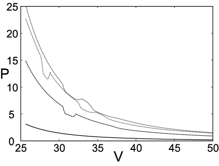
Figure 5: Pressure versus cavity volume. From the bottom to the top, the level number is taken as 1, 19, 38 and 45.

When a disk hit the cavity wall elastically, its momentum is reversed, which is compensated by the impulse on the wall. This is the origin of pressure on the wall. In the classical ideal gas theory, the pressure $P$ is inversely proportional to the volume $V$. In the nonideal gas, on the other hand, there exists a competition between two kind of interactions, namely, the short-range repulsion due to hard cores of constituent molecules and the long-range attractive interaction between them. This competition leads to a peak called van der Waals peak in $P-V$ characteristics. In the quantum two-disk system under consideration, we have both the hard-core repulsion and the strong quantum correlation due to symmetrization of two-disk wavefunctions, and naturally can expect van der Waals-like peaks in $P-V$ characteristics. The pressure $P$ in each excited state taken as an equilibrium is obtained by means of the $\sigma$-dependent eigenvalues. We choose $a=1$, and define the cavity volume as $V=\pi R^{2}$. Then, the pressure is calculated as

$$P=-\frac{dE_{l}}{dV}=-\frac{dE_{l}}{d\sigma}\frac{d\sigma}{dR}\frac{dR}{dV}=\frac{1}{2\pi R^{3}}\frac{dE_{l}}{d\sigma},$$ (16)

where $E_{l}$ stands for the energy for level $l$. Figure 5 shows $P-V$ characteristics for several eigenstates. From the definition (16), the van der Waals-like peaks and pressure fluctuations are attributed to level repulsions. In the low-lying states, there is no van der Waals-like peak, reflecting the absence of level repulsions. In the high-lying states, however, the number of peaks are increased, in contrast to the classical nonideal gas theory that accommodates only a single peak.

A comment should be made here: In the case of a single disk in chaotic billiards like a stadium, one might also see the avoided crossing (AC) and level fluctuations as the system’s parameter is varied. However, it is difficult to find its analogy to the nonideal gas because of the absence of inter-disk interactions. Furthermore, most of chaotic billiards have distorted wall boundary, for which there exists no global pressure as defined in (16) in the case of circle billiard. Thus $P-V$ characteristics and the analogy to the nonideal gas should be meaningful only in the case of interacting particles (disks) confined in the circle billiard.

V Eigenfunction

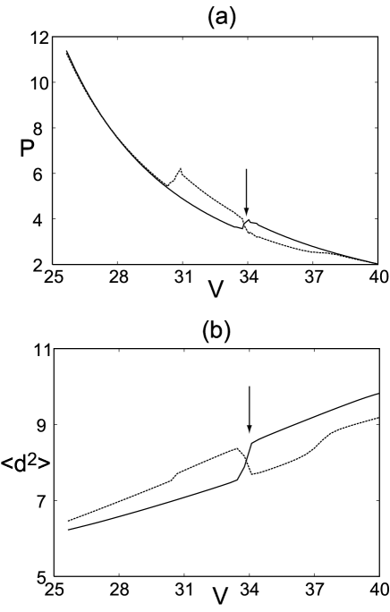
Figure 6: (a) The pressure versus volume for a level $17$ (the solid curve) and $18$ (the dashed curve). (b) Corresponding average of the distance between two disks. The arrow shows the level crossing between these two levels.

The fluctuations of the pressure mentioned above is a promising manifestation of quantum chaos in interacting two-disk systems in the billiard. In this section, we discuss this pressure fluctuation in terms of the wave function.

Although the two disks originally have repulsive correlation due to hard-core interaction, quantum effective exchange interaction gives an additional strong quantum correlation between disks. The averaged distance between disks is determined by the competition between repulsive hard-core interaction and quantum correlation depending on the control parameter $\sigma$. We now wish to make clear whether this competition is responsible for the van der Waals-like peak in quantum systems. For this purpose, we investigate the expectation values of the square distance

$$\langle d^{2}\rangle=\int r_{1}{\rm d}r_{1}r_{2}{\rm d}r_{2}{\rm d}\theta_{1}{\rm d}\theta_{2}\ d^{2}|\psi(r_{1},r_{2},\theta_{1},\theta_{2})|^{2}$$

for each level, where $d=|{\bf r}^{\prime}_{1}-{\bf r}^{\prime}_{2}|$.

We concentrate on typical two neighboring levels employed in Fig. 6 (a), which bear sharp avoided crossings (AC) at the point indicated by the arrow. The avoided level crossing leads to the van-der-Waals-like peak (or dip). In order to study of the origin of this peak, we show the average of the distance between the disks in Fig 6 (b). Clearly, the sharp changes in the pressure curve corresponds to the change in the averaged distance; When the averaged distance increase(decrease) sharply, the pressure increases(decreases) similarly. This result is intuitively reasonable; If the averaged distance increases, the repulsive correlation between disks works strongly, and the existence probability of the disks near the circular wall will increase. Hence, the repulsive correlation contributes to the upward jump in the pressure curve.

VI Summary and discussions

Quantum mechanics of a pair of identical hard disks confined in a circular billiard is investigated. Although the system is circularly symmetric, the short-range interaction between the disks turns out making it nonintegrable and almost chaotic. With use of the two-particle basis wavefunctions that incorporate the excluded volume effect, eigenvalues and eigenfunctions are obtained for various ratios of the radii between each disk and the circle billiard. The energy spectra of eigenvalues versus the disk radius show a multitude of level repulsions. We find the Wigner level spacing distribution in the full range of the disk radius $0<a<R/2$. The Wigner distribution in the vicinity of $a=+0$ should be ascribed to the strong inter-disk repulsion prevailing even at $a=+0$.

The most important feature of this system is a quantal equation of states, i.e., the volume $V$ dependence of the pressure $P$. The tuning of the aspect ratio corresponds to contraction or expansion of the cavity volume $V$. This tuning also changes the pressure $P$ felt by the wall boundary. $P-V$ characteristics shows novel fluctuations coming from quantum level repulsions. The van der Waals-like peaks in this fluctuations are attributed to the competition between the finite size of two disks (responsible for the short-range repulsion) and the quantum-mechanical attractive correlation between them. The expectation values of the square distance between the disks is found to elucidate a mechanism for the pressure fluctuations.

References

- (1) N. S. Krylov, Works on the Foundations of Statistical Physics (Princeton University Press, Princeton, 1979).
- (2) V. I. Arnold and A. Avez, Theorie Ergodique des Systems Dynamiques (Gauthier–Villars, Paris, 1968).
- (3) L. A. Bunimovich and Ya. G. Sinai, Commun. Math. Phys. 78, 479 (1980)
- (4) P. Gaspard, Chaos, Scattering and Statistical Mechanics (Cambridge University Press, Cambridge, 1998).
- (5) P. Gaspard and S. A. Rice, J. Chem. Phys. 90, 2255 (1989).
- (6) A.J. Lichtenberg and M.A. Lieberman, Regular and Stochastic Motion (Springer, Berlin, 1983).
- (7) M.J. Giannoni et al. (eds.), Chaos and Quantum Physics (Session LII, Les Houches, 1989) (Elsevier, Amsterdam, 1991).
- (8) H-J. Stöckmann, Quantum Chaos——An Introduction (Cambridge University Press, Cambridge, 1999).
- (9) A. Awazu, Phys. Rev. E 63, 032102 (2001).
- (10) K.-H. Ahn, K. Richter, and I.-H. Lee, Phys. Rev. Lett. 83, 4144 (1999).
- (11) T. Papenbrock, and T. Prosen, Phys. Rev. Lett. 84, 262 (2000).
- (12) S. Tarucha et al.: Phys. Rev. Lett. 77, 3613 (1996).
- (13) L.P. Kouwenhoven et al., Science 278 (1997) 1788.
- (14) P. Gaspard, and J. R. Dorfman, Phys. Rev. E 52, 3525 (1995).
- (15) P. Gaspard, and H. van Beijeren, J. Stat. Phys. 109, 671 (2002).
- (16) F. Haake, Quantum Signatures of Chaos, 2nd ed. (Springer, Berlin, 2000).
- (17) M. L. Mehta, Random Matrices, 2nd ed. (Academic Press, San Diego, CA, 1991).