Measuring the Density Matrix by Local Addressing

Abstract

We introduce a procedure to measure the density matrix of a material system. The density matrix is addressed locally in this scheme by applying a sequence of delayed light pulses. The procedure is based on the stimulated Raman adiabatic passage (STIRAP) technique. It is shown that a series of population measurements on the target state of the population transfer process yields unambiguous information about the populations and coherences of the addressed states, which therefore can be determined.

Active manipulation of the quantum state of different microscopic systems increases the need for measurement schemes which verify the reliability and efficiency of the engineering procedure. Quantum state reconstruction methods have been proposed in several systems, including light field and matter systems such as the vibrational state of molecules, trapped atom motion, Bose-Einstein condensates, atomic matter waves, electron motion etc., for recent reviews see Refs. ulf ; vogel .

In this work we introduce a procedure to measure the density matrix of a material system. The density matrix is addressed locally in our scheme. More precisely, the measurement process yields a part of the total density matrix, namely the elements

$$\left[\begin{array}[]{ccccc}&\vdots&&\vdots&\\ \cdots&\varrho_{mm}&\cdots&\varrho_{mn}&\cdots\\ &\vdots&&\vdots&\\ \cdots&\varrho_{nm}&\cdots&\varrho_{nn}&\cdots\\ &\vdots&&\vdots&\end{array}\right],$$ (1)

where the indices $m$ and $n$ refer to some steady states of the material system. The procedure is based on population measurements, so one needs an ensemble of identically prepared systems to obtain the required density matrix elements. In practice this means that the measurement is performed for example on an atomic or a molecular beam. A population measurement inevitably entails a reduction of the quantum state, therefore the state of the system is destroyed in the process. The complete density matrix can be determined by repeated application of the measurement procedure for different pairs of states $\{m^{\prime},n^{\prime}\}$. Recently, some new proposals have been published to achieve a similar goal vit1 ; vit2 . We will compare our method with those works at the end of this paper.

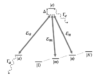
Figure 1: Interaction scheme for the measurement of the density matrix. The states labeled by arabic numbers are occupied, the others are empty initially. The three laser pulses ${\cal E}_{i}(t)$ couple two of the populated states $|m\rangle$ and $|n\rangle$ with the auxiliary state $|a\rangle$ through the excited state $|e\rangle$. A common detuning $\Delta$ is allowed but the three photon resonance is required. The wavy arrows indicate decay from the excited and auxiliary states.

Our measurement procedure is based on the stimulated Raman adiabatic passage (STIRAP) process review . Its implementation imposes the following requirements on the system: the linkage displayed in Fig. 1 must be realizable. We assume that the states labeled by $\{|1\rangle,|2\rangle\,\ldots,|N\rangle\}$ are populated, the others are empty. There are three light pulses $\{{\cal E}_{m}(t),{\cal E}_{n}(t),{\cal E}_{a}(t)\}$ which couple the states $\{|m\rangle,|n\rangle,|a\rangle\}$ via an excited state $|e\rangle$. The other populated states must remain unaffected by these light fields. This could be achieved by exploiting selection rules or selection based on resonance frequencies. The frequencies of the light fields may be detuned by $\Delta$ from the transition frequencies $\omega_{ei}\!=\!(E_{e}-E_{i})/\hbar$, where $E_{i}$ is the energy of the state $|i\rangle\in\{|a\rangle,|1\rangle,\ldots,|N\rangle\}$, but the three-photon resonance condition must be fulfilled.

Initially, the states $|a\rangle$ and $|e\rangle$ are empty. The Master equation which describes the measurement process reads

$$\frac{\partial\hat{\varrho}}{\partial t}\!=\! - \frac{i}{\hbar}[\hat{H}(t),\hat{\varrho}]-\frac{\varGamma_{e}}{2}(|e\rangle\langle e|\hat{\varrho}+\hat{\varrho}|e\rangle\langle e|)$$ (2)

$$- \frac{\varGamma_{a}}{2}(|a\rangle\langle a|\hat{\varrho}+\hat{\varrho}|a\rangle\langle a|),$$

where $\hat{\varrho}$ denotes the density operator of the system. The constants $\varGamma_{e}$ and $\varGamma_{a}$ stand for the decay rates from the states $|e\rangle$ and $|a\rangle$, respectively. The Hamiltonian $\hat{H}(t)$ is given in the interaction picture and the rotating-wave approximation (RWA) as

$$\hat{H}(t)\!=\!\hbar\Delta|e\rangle\langle e|+\frac{\hbar}{2}\sum_{i=m,n,a}(\Omega_{i}(t)|i\rangle\langle e|+h.c.),$$ (3)

where the pulsed Rabi frequency $\Omega_{i}(t)$ derives from the field ${\cal E}_{i}(t)$. The Rabi frequencies $\Omega_{m}(t)$ and $\Omega_{n}(t)$ are taken to have the same envelopes:

$$\Omega_{m}(t)\!=\!\Omega_{p}(t)\cos\alpha,\qquad\Omega_{n}(t)\!=\!\Omega_{p}(t)\sin\alpha\,e^{i\beta},$$ (4)

where $\alpha$ and $\beta$ are fixed angles which define the relative amplitudes and phase of the two pulses, respectively. The pulses $m,n$ and $a$ are delayed with respect to each other; however, for an efficient STIRAP process they must have a significant overlap. In the following $\Omega_{p}(t)$ and $\Omega_{a}(t)$ will be taken real.

Let us neglect the dissipative terms in the Master equation (2). Then we have a purely unitary evolution. Now, our aim is to determine the time evolution operator $\hat{U}(t)$ which governs the time development of the density operator in the absence of dissipation. It will help us understand the essence of the measurement procedure, and we later return to the discussion of dissipations.

The measurement procedure consists of performing a STIRAP process in which a part of the population from the states $|m\rangle$ and $|n\rangle$ is transferred to the state $|a\rangle$. The pulses $m,n$, which act on the states $\{|m\rangle,|n\rangle\}$, play the role of the pump pulses, whereas the pulse $a$ corresponds to the Stokes pulse. It is assumed that they arrive in the counterintuitive time order. The pump pulses $m,n$ define a coupled state (or bright state)

$$|C\rangle\!=\!\cos\alpha\,|m\rangle+\sin\alpha\,e^{i\beta}|n\rangle,$$ (5)

and an orthogonal decoupled state (or dark state)

$$|D\rangle\!=\!-\sin\alpha\,|m\rangle+\cos\alpha\,e^{i\beta}|n\rangle,$$ (6)

see Ref. ari . The Hamiltonian in Eq. (3) can be expressed in terms of the states $|C\rangle$ and $|D\rangle$ to obtain

$$\hat{H}(t)\!=\!\hbar\Delta|e\rangle\langle e|+\frac{\hbar}{2}(\Omega_{p}(t)|C\rangle\langle e|+\Omega_{a}(t)|a\rangle\langle e|+h.c.).$$ (7)

Obviously, the Hamiltonian does not act on the decoupled state $|D\rangle$. From this formulation it can clearly be seen that we have in fact an ordinary STIRAP process defined on a three-state system. The dark state $|\psi_{0}(t)\rangle$ of the Hamiltonian in Eq. (7) is given by

$$|\psi_{0}(t)\rangle\!=\cos\theta|C\rangle-\sin\theta|a\rangle,$$ (8)

and the two bright states are

$$|\psi_{+}(t)\rangle\! = \sin\varphi\sin\theta|C\rangle+\sin\varphi\cos\theta|a\rangle+\cos\varphi|e\rangle$$

$$|\psi_{-}(t)\rangle\! = \cos\varphi\sin\theta|C\rangle+\cos\varphi\cos\theta|a\rangle-\sin\varphi|e\rangle,$$

where the angles $\theta$ and $\varphi$ are defined as

$$\tan\theta\!=\!\frac{\Omega_{p}(t)}{\Omega_{a}(t)},\qquad\tan 2\varphi\!=\!\frac{\Omega(t)}{\Delta},$$ (10)

with $\Omega(t)\!=\!\sqrt{\Omega_{p}^{2}(t)+\Omega_{a}^{2}(t)}$, see Ref. review . In the adiabatic limit, a simple calculation shows that the unitary time evolution operator $\hat{U}(t)$ reads

$$\hat{U}(t)\!= |D\rangle\langle D|+|\psi_{0}(t)\rangle\langle C|$$ (11)

$$+\exp\left(-\frac{i}{\hbar}\int_{-\infty}^{t}\varepsilon_{+}(t^{\prime})dt^{\prime}\right)|\psi_{+}(t)\rangle\langle\psi_{+}(-\infty)|$$

$$+\exp\left(-\frac{i}{\hbar}\int_{-\infty}^{t}\varepsilon_{-}(t^{\prime})dt^{\prime}\right)|\psi_{-}(t)\rangle\langle\psi_{-}(-\infty)|,$$

where $\varepsilon_{+}(t)\!=\!\frac{\hbar}{2}\Omega(t)\cot\varphi$ and $\varepsilon_{-}(t)\!=\!-\frac{\hbar}{2}\Omega(t)\tan\varphi$ are the two nonzero eigenenergies of the Hamiltonian Eq. (7). The physical interpretation of this result is quite simple: The decoupled state $|D\rangle$ remains untouched throughout the transfer process. The coupled state $|C\rangle$ follows adiabatically the dark state $|\psi_{0}(t)\rangle$ of the Hamiltonian $\hat{H}(t)$ [Eq. (7)]. The bright states $|\psi_{\pm}(t)\rangle$ also evolve adiabatically, however, they acquire a phase shift because they belong to nonzero eigenenergies $\varepsilon_{\pm}(t)$.

In the adiabatic limit, the bright states $|\psi_{\pm}(t)\rangle$ are not populated throughout the whole time, provided that initially they were not populated. Thus, we have found that the final state of the system, after the pulses have passed becomes

$$\lim_{t\rightarrow\infty}\hat{U}(t)\hat{\varrho}_{i}\hat{U}^{{\dagger}}(t) = \!|D\rangle\langle D|\hat{\varrho}_{i}|D\rangle\langle D|+|a\rangle\langle C|\hat{\varrho}_{i}|C\rangle\langle a|$$ (12)

$$- |D\rangle\langle D|\hat{\varrho}_{i}|C\rangle\langle a|-|a\rangle\langle C|\hat{\varrho}_{i}|D\rangle\langle D|.$$

Let us suppose that we are able to measure the population $P_{a}$ on the state $|a\rangle$. Then, the result can be expressed in terms of the density matrix elements $(\hat{\varrho}_{i})_{mm}$, $(\hat{\varrho}_{i})_{nn}$, $(\hat{\varrho}_{i})_{mn}$ as

$$P_{a}\!=\!\langle C|\hat{\varrho}_{i}|C\rangle\! = \!\cos^{2}\alpha\,(\hat{\varrho}_{i})_{mm}+\sin^{2}\alpha\,(\hat{\varrho}_{i})_{nn}$$ (13)

$$+ \sin 2\alpha\,\text{Re}\{(\hat{\varrho}_{i})_{mn}\,e^{i\beta}\},$$

where we have made use of the definition Eq. (5). The outcome of the measurement is phase sensitive: It depends on the relative phase $\beta$ between the fields $m$ and $n$ (cf. Eq. (4)). Observe, that the coherence $(\hat{\varrho}_{i})_{mn}$ also appears, so one expects that by accomplishing an appropriate series of measurements one can obtain not only the diagonal elements of the density matrix, but the coherences as well. Indeed, the three required density matrix elements can be determined in four steps: In the first and second measurements, one of the pump field $n$ or $m$ is switched off which corresponds to taking $\alpha\!=\!0$ or $\alpha\!=\!\pi/2$. In this way, we get the diagonal density matrix elements $(\hat{\varrho}_{i})_{mm}$ and $(\hat{\varrho}_{i})_{nn}$. In the third and fourth steps, both of the pump fields $m$ and $n$ are present so that the value of $\alpha$ is chosen as $0\!<\!\alpha\!<\!\pi/2$. One measurement is performed with the choice $\beta\!=\!0$ and an other with $\beta\!=\!-\pi/2$. It is easy to show, that by combining the results of the last two measurements with that of the first and second, one can unambiguously determine the needed $(\hat{\varrho}_{i})_{mn}$.

There is one question left, which we have to answer: How can one measure the population $P_{a}$? Here we return back to the analysis of the dissipation mechanisms which we have postponed so far. Let us consider again the Master equation (2). If the usual STIRAP conditions are met during the measurement procedure, then the decay from the excited state $|e\rangle$ has got negligible effect, since this state is minimally populated glushko ; vit3 . The situation is quite different in the case of the decay from the target state $|a\rangle$: This state is deeply involved in the transfer process. The dissipation may influence significantly the population transfer to the target state and as a result, it deteriorates the fidelity of the measurement. However, it can also be utilized to monitor the population on the target state $|a\rangle$.

It is plausible to assume, that the decay rate from the state $|a\rangle$ to the states $|m\rangle$ and $|n\rangle$ is negligibly small, since they have the same parity, because both of the transitions $|m\rangle\leftrightarrow|e\rangle$ and $|e\rangle\leftrightarrow|a\rangle$ are dipole allowed; the argument is the same in the case of the state $|n\rangle$. The decay from the state $|a\rangle$ to the state $|e\rangle$ is undesirable. It can be avoided if the energy of the state $|a\rangle$ is lower than that of the state $|e\rangle$ or if there are faster decay channels. In the following we assume that the decay between these states is negligible.

Now we present a simplified treatment of the dissipation from the target state $|a\rangle$ by assuming that the initial state of the system can be given by a state vector $\boldsymbol{B}\!=\![B_{C},B_{e},B_{a}]^{T}$ in the basis $\left\{|C\rangle,|e\rangle,|a\rangle\right\}$. Note that in this definition we have included only those states of the system which participate in the population transfer process. This means that the norm of $\boldsymbol{B}$ may be smaller than unity. The Master equation (2) is replaced by a Schrödinger equation with a non-Hermitian Hamiltonian. In the adiabatic basis Eqs. (8) and (Measuring the Density Matrix by Local Addressing), the Schrödinger equation reads

$$i\frac{d}{dt}\boldsymbol{A}(t)=\boldsymbol{H}^{\prime}(t)\boldsymbol{A}(t),$$ (14)

where the effective non-Hermitian Hamiltonian $\boldsymbol{H}^{\prime}(t)$ is given by

$$\boldsymbol{H}^{\prime}(t)\!=\!\left[\begin{array}[]{ccccc}\frac{1}{2}\Omega\cot\varphi-i\varGamma_{a}\cos^{2}\theta\sin^{2}\varphi&&i\left(\frac{1}{2}\varGamma_{a}\sin(2\theta)+\dot{\theta}\right)\sin\varphi&&-i\frac{1}{2}\varGamma_{a}\cos^{2}\theta\sin(2\varphi)+i\dot{\varphi}\\ \\ i\left(\frac{1}{2}\varGamma_{a}\sin(2\theta)-\dot{\theta}\right)\sin\varphi&&-i\varGamma_{a}\sin^{2}\theta&&i\left(\frac{1}{2}\varGamma_{a}\sin(2\theta)-\dot{\theta}\right)\cos\varphi\\ \\ -i\frac{1}{2}\varGamma_{a}\cos^{2}\theta\sin(2\varphi)-i\dot{\varphi}&&i\left(\frac{1}{2}\varGamma_{a}\sin(2\theta)+\dot{\theta}\right)\cos\varphi&&\frac{1}{2}\Omega\tan\varphi-i\varGamma_{a}\cos^{2}\theta\cos^{2}\varphi\end{array}\right].$$ (15)

Decay from the excited state $|e\rangle$ is neglected in order to obtain more simple expressions. This approximation is justified by the small involvement of the excited state and by assuming small decay rate $\varGamma_{e}$. The state vector $\boldsymbol{B}(t)$ is transformed by the orthogonal rotation

$$\boldsymbol{O}(t)\!=\!\left[\begin{array}[]{ccc}\sin\varphi\sin\theta&\cos\theta&\cos\varphi\sin\theta\\ \cos\varphi&0&-\sin\varphi\\ \sin\varphi\cos\theta&-\sin\theta&\cos\varphi\cos\theta\end{array}\right]$$ (16)

according to

$$\boldsymbol{A}(t)\!=\!\boldsymbol{O}^{-1}(t)\boldsymbol{B}(t).$$ (17)

In Eq. (15) one can see that the decay from the target state $|a\rangle$ affects the time evolution both of the dark state and the bright states. More precisely, terms proportional to $\varGamma_{a}$ appear not only on the diagonal but also on the off-diagonal part of the Hamiltonian. On one hand, these terms lead to a decrease of the probability amplitudes for all of the three adiabatic states; on the other hand, they contribute to nonadiabatic couplings which mix the adiabatic states among themselves. If $\Omega_{{\rm max}}\!\gg\!\varGamma_{a}$ and the process is adiabatically slow, then the diagonal elements dominate over the nondiagonal ones in Eq. (15). Then the states $|\psi_{+}(t)\rangle$ and $|\psi_{-}(t)\rangle$ can be adiabatically eliminated by setting $\dot{A}_{+}(t)\!=\!\dot{A}_{-}(t)\!=\!0$ in Eq. (14) and solving the resulting algebraic equations for ${A}_{+}(t)$ and ${A}_{-}(t)$. Thus, by inserting these solutions in the differential equation for ${A}_{0}(t)$ we find the final population $P_{a}(\varGamma_{a})$ on the state $|a\rangle$ to be

$$P_{a}(\varGamma_{a})=$$ (18)

$$P_{a}\exp\left[-2\varGamma_{a}\int_{-\infty}^{\infty}\displaylimits\frac{\Delta^{2}\dot{\theta}^{2}\cos^{2}\theta+(\Omega^{2}/4+\dot{\varphi}^{2})^{2}\sin^{2}\theta}{\Delta^{2}\varGamma_{a}^{2}\cos^{4}\theta+(\Omega^{2}/4+\dot{\varphi}^{2})^{2}}dt\right],$$

since $P_{a}(\varGamma_{a})\!=\!|A_{0}(\infty)|^{2}$. The symbol $P_{a}$ denotes the initial population on the state $|C\rangle$ which is given by Eq. (13). In the absence of decay $\varGamma_{a}\!=\!0$, we recover the result derived earlier. For a significantly large decay rate $\varGamma_{a}$, the target state $|a\rangle$ is emptied by the end of the population transfer process. If the decay is accompanied by emission of photons, then the signal will be proportional to the population $P_{a}$.

In general, the initial state of the system cannot be described by a state vector. In this case, our considerations in the preceding paragraphs cannot be applied straightforwardly. However, some results are still valid: In the Master equation (2) the projection of the density operator $\hat{\varrho}$ on the decoupled state $|D\rangle$ is a conserved quantity during the transfer process. This implies that the maximum amount of population which can be transferred to the target state $|a\rangle$ is given by $P_{a}$ in Eq. (13). Therefore, we have performed a numerical simulation, whose main purpose is to verify whether this portion is indeed transferred. The simulation may also allow us to study the adiabaticity of the process: the excited state must be involved only minimally in the population transfer. As a result we have verified numerically, for a wide range of $\varGamma_{a}$ and for several initial density operators $\hat{\varrho}_{i}$, that the population $\langle C|\hat{\varrho}_{f}|C\rangle$ is zero and the population on the excited state $|e\rangle$ is very small throughout the whole time. The quantity $\langle C|\hat{\varrho}_{f}|C\rangle$ is obtained from the simulation in the presence of decay from the state $|a\rangle$. The parameters of the simulation have been chosen as follows: The atomic system is described by $(\Delta,\varGamma_{e},\varGamma_{a})\!=\!(0.3,0.1,0.0-3.0)$; the pulses have been Gaussian with parameters $(\Omega_{{\rm max}},T,\tau)\!=(6.0,2.0,3.2)$, where $T$ denotes the half-width of the pulses, and $\tau$ is the pulse delay. Time and frequency are measured in arbitrary units.

In this way we have shown that combining a STIRAP process with a population measurement on the target state of the population transfer, yields the expectation value of the operator

$$\hat{V}\! = \!\cos^{2}\alpha\,|m\rangle\langle m|+\sin^{2}\alpha\,|n\rangle\langle n|$$ (19)

$$+ \sin\alpha\,\cos\alpha(e^{i\beta}|m\rangle\langle n|+e^{-i\beta}|n\rangle\langle m|).$$

Performing a series of measurements of this kind by varying the angles $\alpha$ and $\beta$, the density matrix elements $(\hat{\varrho}_{i})_{mm}$, $(\hat{\varrho}_{i})_{nn}$, and $(\hat{\varrho}_{i})_{mn}$ can be unambiguously obtained. In Refs. vit1 ; vit2 a measurement procedure has been proposed where the population from the ground state ensemble is transferred to an excited state. This scheme seems more sensitive to the decay from the excited state because it gets significantly populated during the process. Therefore, the incoherent decay back to the ground states may interrupt the coherent evolution which is required in this measurement procedure as well.

In conclusion we have worked out a measurement procedure based on stimulated Raman adiabatic passage to obtain the the density matrix elements of a material system. The scheme is highly reliable due to the robustness of the STIRAP process. In the beginning of the measurement, a part of the density operator is expressed using two orthogonal states: the coupled and the decoupled states, which are defined by the two pump pulses. In this way a $2\times 2$ block of the density matrix is addressed. The coupled part of the density operator is then transferred to an auxiliary state. We have shown that by measuring the population on the auxiliary state for some configurations of the pump pulses, the $2\times 2$ block of the density matrix can be determined.

The measurement procedure presented here can be used efficiently when it is not necessary to obtain the complete density operator, but only few elements are needed. We propose the implementation of this scheme in several microscopic quantum systems, e.g. electronic states of atoms, vibronic states of molecules etc..

This work was supported by the European Union Research and Training Network COCOMO, contract HPRN-CT-1999-00129.

References

- (1) U. Leonhardt, Measuring the Quantum State of Light, (Cambridge University Press, Cambridge, 1997).
- (2) D.G. Welsch, W. Vogel, and T. Opatný, Progress in Optics XXXIX, ed. E. Wolf, (Elsevier Science, 1999).
- (3) N.V. Vitanov, B.W. Shore, R.G. Unanyan, and K. Bergmann, Opt. Coomun. 179, 74 (2000).
- (4) N.V. Vitanov, J. Phys. B: At. Mol. Opt. Phys. 33, 2333 (2000).
- (5) STIRAP has been recently reviewed in K. Bergmann, H. Theuer, and B.W. Shore, Rev. Mod. Phys. 70, 1003 (1998) and N.V. Vitanov, M. Fleishhauer, B.W. Shore, and K. Bergmann, Adv. At. Mol. Opt. Phys. (in press).
- (6) For a review of dark states, see E. Arimondo, in Progress in Optics ed. E. Wolf, vol. 35 (Elsevier, Amsterdam, 1996) p. 257.
- (7) B. Glushko and B. Kryzhanovsky, Phys. Rev. A 46, 2823 (1992).
- (8) N.V. Vitanov and S. Stenholm, Phys. rev. A 56, 1463 (1997).