On the Quantum Computational Complexity of the Ising Spin Glass Partition Function and of Knot Invariants

Abstract

It is shown that the canonical problem of classical statistical thermodynamics, the computation of the partition function, is in the case of $\pm J$ Ising spin glasses a particular instance of certain simple sums known as quadratically signed weight enumerators (QWGTs). On the other hand it is known that quantum computing is polynomially equivalent to classical probabilistic computing with an oracle for estimating QWGTs. This suggests a connection between the partition function estimation problem for spin glasses and quantum computation. This connection extends to knots and graph theory via the equivalence of the Kauffman polynomial and the partition function for the Potts model.

I Introduction

Feynman famously conjectured that unlike classical computers, quantum computers should be efficient at simulating quantum mechanics Feynman:QC ; Feynman:QC1 . This was verified by Lloyd Lloyd:96 , and further developed by several other authors, who demonstrated exponential speedup over the best known classical algorithms for a variety of quantum mechanical problems such as solution of the constant potential Schrödinger and Dirac equations using lattice gas automata Meyer:96 ; Meyer:97 ; Boghosian:97c ; Boghosian:97a , solution of the Schrödinger equation in the circuit model Wiesner:96 ; Zalka ; Zalka:98 , simulation of fermionic systems Abrams:97 ; Ortiz:00 , computation of the thermal rate constant of chemical reactions Lidar:98RC , computation of correlation functions Terhal:00 , simulation of topological field theories Freedman:00 , and simulation of pairing Hamiltonians such as the BCS model WuByrdLidar:01 . A naturally related question is whether quantum computers can efficiently solve problems in classical physics. This question was first raised, and partially answered, in the context of Ising spin glasses Lidar:PRE97a . It has recently received renewed attention in the context of hydrodynamics Yepez:01 ; Meyer:02 (with polynomial speedups), chaos Georgeot:01a ; Georgeot:01b ; Terraneo:03 (with exponential speedups, though some of these have been challenged Zalka:01 ), and knot theory Kauffman:01 (so far without speedup), which has a deep connection to classical statistical mechanics Kauffman:book .

Here we revisit classical Ising spin glasses and also address knot theory. The canonical problem of classical statistical thermodynamics is the calculation of the partition function $Z$. For a system in thermodynamic equilibrium, if the partition function is known, one can obtain exact results for all thermodynamic quantities such as the magnetization, susceptibility and specific heat. Models for which analytical calculations of this type can be performed include a variety of one dimensional (1D) models and the 2D Ising model Onsager44 ; Baxter:book . However, for most systems of interest, including the 3D Ising model and most Ising spin glass models, no analytical calculation of the partition function is available Green . We consider classical spin systems, in particular the Ising model Ising in which each spin has two states $\sigma_{i}=\pm 1$, and spins interact pairwise with an interaction energy of the form $J_{ij}\sigma_{i}\sigma_{j}$. From a computational complexity perspective this provides a rich class of problems. In particular, the problem of finding the ground state of the short range 3D Ising spin glass (quenched random $J_{ij}$), as well as the fully antiferromagnetic (all $J_{ij}=-|J|$) 2D Ising model in the presence of a constant magnetic field was shown by Barahona to be NP-hard, by a mapping to problems in graph theory. On the other hand, it is known that there exists a fully polynomial randomized approximation scheme for the ferromagnetic Ising model (all $J_{ij}=|J|$), on arbitrary graphs Jerrum:90 .

The problem of sampling from the Gibbs distribution of the $J_{ij}=\pm J$ (with random signs) spin glass on a quantum computer was addressed in Lidar:PRE97a . A linear-time algorithm was found for the construction of the Gibbs distribution of configurations in the Ising model, including partially frustrated models. A magnetic field can be incorporated as well without increase in the run-time. The algorithm was designed so that each run provides one configuration with a quantum probability equal to the corresponding thermodynamic weight. I.e., the probabilities of measuring states are ordered by the energies of the corresponding spin configurations, with the ground state having the highest probability. Therefore the partition function is approximated efficiently and statistical averages needed for calculations of thermodynamic quantities obtained from the partition function, are approximated in the fastest converging order in the number of measurements. Unlike Monte Carlo simulations on a classical computer, consecutive measurements on a quantum computer can be totally uncorrelated. Thus the algorithm neither suffers from critical slowing down (a polynomial slowdown in Monte Carlo moves associated with large correlated spin clusters forming near the critical temperature) Swendsen87 , nor gets stuck in local minima. This uniform performance is an advantage over the best known classical algorithms, which are tailored to specific lattices or graphs Swendsen87 . However, the main problem of the algorithm is the limited control it offers in the construction of a specific realization of bonds on the Ising lattice. Indeed, since the run-time of the algorithm is linear, it is reasonable to suspect that it cannot simulate a hard instance of an Ising spin glass.

A completely different approach to sampling from the Gibbs distribution for the ferromagnetic Ising model was recently developed by Nayak, Schulman and Vazirani (NSV) Nayak:unp , which however does not appear to provide a speedup over the best known classical algorithm Randall:99 . The VNS algorithm for the ferromagnetic Ising model uses an interesting representation of the partition function as a discrete Fourier transform, in conjunction with a Markov chain sampling procedure. Two of the main results of the present paper are (i) the generalization of this Fourier transform representation to the $\pm J$ spin glass case, (ii) (the central result) a connection of this representation to certain simple sums known as “quadratically signed weight enumerators” (QWGTs). Let us now motivate the importance of result (ii).

In virtually all previous work on simulation of physical systems on quantum computers Lloyd:96 ; Meyer:96 ; Meyer:97 ; Boghosian:97c ; Boghosian:97a ; Wiesner:96 ; Zalka ; Zalka:98 ; Abrams:97 ; Ortiz:00 ; Lidar:98RC ; Terhal:00 ; Freedman:00 ; WuByrdLidar:01 ; Lidar:PRE97a ; Yepez:01 ; Meyer:02 ; Georgeot:01a ; Georgeot:01b ; Terraneo:03 ; Zalka:01 ; Kauffman:01 , the approach pursued was one of attempting to find a concrete algorithm for a specific simulation problem. A fruitful alternative is to consider instead the question of the complexity class that the simulation problem belongs to. We do this here by following a lead due to the Knill and Laflamme (KL): KL showed that quantum computing is polynomially equivalent to classical probabilistic computing with an oracle for estimating QWGTs Knill:01a . Combined with our results (i),(ii), this suggests that the quantum computational complexity of sampling from the Gibbs distribution for the Ising spin glass problem can be understood in terms of QWGTs. However, we have unfortunately not yet been able to establish the connection at this level. Nevertheless, the possibility of a (spin glass)-(QWGTs)-(quantum computation) connection is sufficiently tantalizing to point it out in detail. We hope that by expressing the partition function as a QWGT we have taken the first step in a direction that will allow future research to explore the important question of the quantum computational complexity of the Ising spin glass problem.

In fact, the connections do not end here. There is a rich inter-relation between classical statistical mechanics and topology, in particular the theory of classification of knots. The first such connection was established by Jones Jones:89 , who discovered knot invariants (the Jones’ polynomial) during his investigation of topological properties of braids Jones:85 . It is known that classical evaluation of the Jones’ polynomial is #P-hard Jaeger:90 . The connection between knots and models of classical statistical mechanics was greatly embellished by Kauffman Kauffman:book . Here we will exploit this connection to show [our main result (iii)] that the evaluation of another knot invariant, the Kauffman polynomial, can also be cast in some cases as a QWGT evaluation problem. Thus a quantum algorithm for QWGT evaluation should shed light on the quantum computational complexity of knot invariants, a subject which has been explored by Freedman et al. Freedman:01 and by Kauffman and Lomonaco Lomonaco . Knot invariants are, in turn, also tightly related to graph theory; e.g., the graph coloring problem can be considered an instance of evaluation of the Kauffman polynomial, via the Tutte polynomial Kauffman:book .

Mathematically, the reason that these seemingly unrelated subjects are all inter-related is due to the fact that key properties can be expressed, in all cases, in terms of certain polynomials. While these polynomials originate from widely distinct problems, from the point of view of computational complexity their evaluation is one and the same problem, much in the same spirit as the fact that solving one problem in the class of NP-complete problems solves them all Papadimitriou:book . The present work contributes to this unification.

The structure of this paper is as follows. In Sec. II we derive our first main result: we rewrite the Ising spin glass partition function for an arbitrary graph as a discrete Fourier transform. This motivates the consideration of the partition function evaluation problem in terms of its computational complexity, which we formalize in Sec. III. We then review QWGTs in Sec. IV. In Section V we derive our second main result: the connection between the evaluation of the Ising spin glass partition function and QWGTs. In Sec. VI we continue the program of connecting disparate objects to the problem of QWGT evaluation, and obtain our third main result: we show that the Kauffman polynomial too can be expressed a QWGT. We do this after first reviewing the connection between knots and classical statistical mechanics. Section VII concludes. Some further observations concerning the representation of the partition function are collected in Appendix A.

II Fourier Transform Representation of the Partition Function

Let $G=(E,V)$ be a finite, arbitrary undirected graph with $|E|$ edges and $|V|$ vertices. Identify each vertex $i\in V$ with a classical spin ($\sigma_{i}=\pm 1$) and each edge $(i,j)\in E$ with a bond ($J_{ij}=\pm J$). Denote a given spin configuration by $\sigma=(\sigma_{1},\sigma_{2},...,\sigma_{|V|})$ and a bond configuration by $(J_{12},...,J_{ij},...)$. We assume that the bond configuration is chosen at random and then remains fixed (“quenched randomness”). The Hamiltonian of the system is

$$H(\sigma)=-\sum_{(i,j)\in E}J_{ij}\sigma_{i}\sigma_{j}.$$ (1)

(We remark on the case with a magnetic field in Appendix A.1.) The probability of the spin configuration $\sigma$ in thermal equilibrium at temperature $T$ is given by the Gibbs distribution:

$$P(\sigma)={\frac{1}{Z}}W(\sigma),$$ (2)

where the Boltzmann weight is

$$W(\sigma)=\exp[-\beta H(\sigma)],$$ (3)

$\beta=1/kT$ is the inverse temperature, and $Z$ is the partition function:

$$Z(\{J_{ij}\})=\sum_{\sigma}\exp[-\beta H(\sigma)].$$ (4)

Now note the identity

$$e^{x}=\cosh(x)[1+\tanh(x)]$$ (5)

and use it to rewrite the Boltzmann weight (3) as

$$W(\sigma)=\prod_{(i,j)\in E}\cosh(\beta J_{ij}\sigma_{i}\sigma_{j})[1+\tanh(\beta J_{ij}\sigma_{i}\sigma_{j})].$$ (6)

Let

$$J_{ij}=q_{ij}J,$$ (7)

where $q_{ij}=\pm 1$ is a quenched random variable. Since $\cosh(x)=\cosh(-x)$ and $\tanh(x)=-\tanh(-x)$ we find

$$W(\sigma)=\Theta\prod_{(i,j)\in E}(1+q_{ij}\sigma_{i}\sigma_{j}\lambda),$$ (8)

where

$$\Theta={[\cosh(\beta J)]^{|E|},}$$ (9)

and

$$\lambda=\tanh(\beta J).$$ (10)

Next expand out the product to obtain

$$P(\sigma) = \Theta[1+\lambda\sum_{(i,j)\in E}\sigma_{i}q_{ij}\sigma_{j}$$ (11)

$$+\lambda^{2}\sum_{(i,j),(k,l)\in E}(\sigma_{i}q_{ij}\sigma_{j})(\sigma_{k}q_{kl}\sigma_{l})+....]$$

Note that $\lambda^{k}$ is the coefficient in front of a sum containing $k$ bonds $q_{ij}$, which are not necessarily all connected. For example, the term $q_{ij}\sigma_{i}\sigma_{j}q_{kl}\sigma_{k}\sigma_{l}$ where all indexes differ represents two unconnected bonds (Fig. 1a), whereas if $j=k$ the same term represents two connected bonds sharing one spin (Fig. 1b). Let $b\subseteq E$ denote such a subgraph, with $k=|b|$ edges. There are $\binom{|E|}{|b|}$ ways of choosing subgraphs with $|b|$ edges. Thus the total number of subgraphs is:

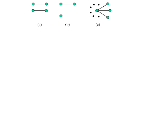
Figure 1: Illustration of subgraphs.

$$\sum_{|b|=0}^{|E|}\binom{|E|}{|b|}=2^{|E|}.$$ (12)

This suggests to label the subgraphs in a binary fashion (to be explained below): Let $b=(b_{1},b_{2},...,b_{|E|})$ (where $b_{j}\in\{0,1\}$) be the binary number of subgraph $b$. The numbering is such that $b_{j}=1$ ($0$) indicates the presence (absence) of edge number $j$ of $G$. Further, we will use the convention that first all $|E|$ single-edge subgraphs are counted (i.e., vectors $b$ with a single $1$ entry, all the rest $0$), then all $\binom{|E|}{2}$ double-edge subgraphs (vectors $b$ with two $1$ entries, all the rest $0$), etc. Thus, e.g., $b=(0,0,...,0,1)$ could corresponds to the subgraph containing only the first edge (or bond): $J_{12}$, whereas $b=(0,0,...0,1,0,1)$ could correspond to the subgraph containing only $J_{12}$ and $J_{34}$. Note that $|b|$ is the Hamming weight of $b$. Since the total number of subgraphs is $2^{|E|}$, the above numbering scheme is a one-to-one covering of the subgraph space, and moreover, the subgraphs are labeled in increasing order of $|b|$.

Next note that in Eq. (11), a spin $\sigma_{i}$ may appear more than once in sums of order $k\geq 2$, in fact as many times as the number of bonds emanating from $\sigma_{i}$, which we denote by $\mathrm{deg}_{b}(i)$. Then $\sigma_{i}^{\mathrm{deg}_{b}(i)}$ is the contribution of spin $i$ in subgraph $b$ to the product in the sum of order $k=|b|$ in Eq. (11). Collecting all the observations above, it follows that Eq. (11) can be rewritten as:

$$P(\sigma)=\Theta\sum_{b}\lambda^{|b|}\prod_{i\in V(b)}\sigma_{i}^{\mathrm{deg}_{b}(i)}\prod_{(i,j)\in b}q_{ij}.$$ (13)

Here $V(b)$ denotes the set of vertices in subgraph $b$.

Next introduce the parity vector ${\alpha}^{b}=(\alpha_{1}^{b},\alpha_{2}^{b},...,\alpha_{|V|}^{b})$ of a subgraph, with components $\alpha_{i}^{b}=1$ if ($i\in V(b)$ and $\mathrm{deg}_{b}(i)$ is odd), $\alpha_{i}^{b}=0$ otherwise. Then clearly $\sigma_{i}^{\mathrm{deg}_{b}(i)}=\sigma_{i}^{\alpha_{i}^{b}}$. At this point it is more convenient to transform to a binary representation for the spins as well. Let:

$$s_{i}={\frac{1-\sigma_{i}}{2}}$$ (14)

be the components of the binary vector of spin values $s=(s_{1},s_{2},...,s_{|V|})$. We have $\sigma_{i}=(-1)^{s_{i}}$ so that $\sigma_{i}^{\mathrm{deg}_{b}(i)}=(-1)^{\alpha_{i}^{b}s_{i}}$. Therefore:

$$\prod_{i\in V(b)}\sigma_{i}^{\mathrm{deg}_{b}(i)}=(-1)^{{\alpha}^{b}\cdot s},$$ (15)

where “$\cdot$” stands for the (mod 2) bit-wise scalar product. The same change can be affected for the bonds by introducing:

$$w_{ij}={\frac{1-q_{ij}}{2}},$$ (16)

so that the binary vector $w=(w_{12},w_{13},...)$ of length $|E|$ specifies whether edge $(i,j)$ supports a ferromagnetic ($w_{ij}=0$) or antiferromagnetic ($w_{ij}=1$) bond. Again, $q_{ij}=(-1)^{w_{ij}}$, so that:

$$\prod_{(i,j)\in b}q_{ij}=(-1)^{b\cdot w}.$$ (17)

Using Eqs. (15),(17) in Eq. (13) it is now possible to rewrite the Boltzmann weight of a particular spin configuration $s$ as:

$$W(s)=\Theta\sum_{b}\lambda^{|b|}(-1)^{{\alpha}^{b}\cdot s+b\cdot w}.$$ (18)

Now, the partition function is just the sum over all spin configurations. Using Eq. (18) we thus find:

Proposition 1

The spin-glass partition function is a double discrete Fourier (or Walsh-Hadamard) transform, over the spin and subgraph variables:

$$Z(w)=\Theta\sum_{s}\sum_{b}\lambda^{|b|}(-1)^{{\alpha}^{b}\cdot s+b\cdot w}.$$ (19)

Note that the sum over $s$ extends over $2^{|V|}$ terms, while the sum over $b$ extends over $2^{|E|}$ terms. By changing the order of summation, the sum over $s$ can actually be carried out, since:

$$\sum_{s}(-1)^{{\alpha}^{b}\cdot s}=2^{|V|}\delta_{({\alpha}^{b},0)},$$ (20)

where $\delta$ is the Kronecker symbol. A systematic procedure for finding the parity vectors from the subgraphs vectors uses the incidence matrix $A$. For any graph $G=(E,V)$ this matrix is defined as follows ($v\in V$) Wilson:book :

$$A_{v,(i,j)}=\left\{\begin{array}[]{ll}1&\mbox{$(v=i\>\>{\rm and}\>\>(i,j)\in E)$}\\ 0&\mbox{${\rm else}$}\end{array},\right.$$ (21)

so $A$ is a $|V|\times|E|$ matrix of $0$’s and $1$’s. It is well known that given $G$ and a specific subgraph $b$ Wilson:book ,

$${\alpha}^{b}=A\cdot b.$$ (22)

Combining Eqs. (9),(10),(19),(20),(22), we finally have:

$$Z(w)={\frac{2^{|V|}}{(1-\lambda^{2})^{|E|/2}}}\sum_{b:\,A\cdot b=0}\lambda^{|b|}(-1)^{b\cdot w}.$$ (23)

In words, the sum over the subgraphs includes only those with zero overall parity, i.e., those having an even number of bonds emanating from all spins. This immediately implies that “dangling-bond” subgraphs are not included in the sum. We note that $Z(w)$ can also be rewritten as a power series in $\lambda$, which is useful for a high-temperature expansion; this is discussed in App. A.2. The representation (23) allows us to establish a direct connection with QWGTs, which is the subject of the quantum computational complexity of $Z$, to which we turn next.

III Formulating the Computational Complexity of the Ising Spin Glass Partition Function

The most natural computational complexity class for quantum computation is BQP: the class of decision problems solvable in polynomial time using quantum resources (a quantum Turing machine, or, equivalently, a uniform family of polynomial-size quantum circuits) with bounder probability of error Aharonov:98 ; Aaronson-zoopage . The class BQPP is the natural generalization of BQP to promise problems Knill:01a . Relative to the polynomial hierarchy of classical computation, it is known that BPP$\subseteq$BQP$\subseteq$PP$\subseteq$PSPACE, but none of these inclusions is known to beproper Adleman:97 .

In order to address the quantum computational complexity of the spin glass partition function we define:

Definition 1

An instance of the Ising spin glass problem is the data $\Delta\equiv(G,w,\lambda)$.

Now, let $Z^{\Delta}(s)$ be the partition function for given data $\Delta$ and given spin configuration $s\in\{0,1\}^{|V|}$, and let

$$Z_{k}^{\Delta}(s):\{0,1\}^{N}\rightarrow\{0,1\}$$ (24)

be the $k^{\mathrm{th}}$ digit of $Z^{\Delta}(s)$. Let $\Gamma^{\Delta}(s,k)$ be a quantum circuit that takes as input the spin configuration $s$ and the digit location $k$, for fixed data $\Delta$. Let $W_{\Gamma}=\prod_{i}U_{i}$ be an implementation of $\Gamma^{\Delta}$ in terms of some unitary operators $U_{i}$. Let the circuit be designed so that the answer $Z_{k}^{\Delta}(s)$ is encoded into the state of the first qubit, and let $\Pi_{1}=|0\rangle_{1}\langle 0|$ be the projection onto state $|0\rangle$ of this qubit. Then the probability of measuring the state $|0\rangle_{1}$ after the circuit was executed, starting from the “blank” initial state $|\mathbf{0}\rangle=|0\cdots 0\rangle$, is $\Pr[\Gamma^{\Delta}(s,k)]=\langle\mathbf{0}|W_{\Gamma}^{\dagger}\Pi_{1}W_{\Gamma}|\mathbf{0}\rangle$. We can now define:

Definition 2

$Z_{k}^{\Delta}(s)\in$ BQP if there exists a classical polynomial-time algorithm for specifying $\Gamma^{\Delta}$ such that

$$\Pr[\Gamma^{\Delta}(s,k)] \geq \frac{2}{3}\hskip 8.53581pt\mathrm{if}\hskip 8.53581ptZ_{k}^{\Delta}(s)=0\hskip 28.45274pt\mathrm{and}$$

$$\Pr[\Gamma^{\Delta}(s,k)] \leq \frac{1}{3}\hskip 8.53581pt\mathrm{if}\hskip 8.53581ptZ_{k}^{\Delta}(s)=1.$$

We can then formulate the following open problem:

Problem 1

For which instances $\Delta$ of the Ising spin glass problem is evaluating the partition function in BQP?

A particularly promising way to attack this problem appears to be the connection to QWGTs, which we address next.

IV Quadratically Signed Weight Enumerators

Quadratically signed weight enumerators (QWGTs) were introduced by Knill and Laflamme in Ref. Knill:01a (where “QWGT” is pronounced “queue-widget”). A general QWGT is of the form

$$S(A,B,x,y)=\sum_{b:Ab=0}(-1)^{bBb}x^{|b|}y^{n-|b|}$$ (25)

where $A$ and $B$ are $0,1$-matrices with $B$ of dimension $n\times n$ and $A$ of dimension $m\times n$. The variable $b$ in the summand ranges over $0,1$-column vectors of dimension $n$, and all calculations involving $A$, $B$ and $b$ are done modulo $2$. It should be noted that $|S(A,B,x,y)|\leq(|x|+|y|)^{n}$. In Ref. Knill:01a it was shown that quantum computation is polynomially equivalent to classical probabilistic computation with an oracle for estimating the value of certain QWGTs with $x$ and $y$ rational numbers. In other words, if these sums could be evaluated, one could use them to generate the quantum statistics needed to simulate the desired quantum system.

More specifically, let $I$ be the identity matrix, $\mathrm{diag}(A)$ the diagonal matrix whose diagonal is the same as that of $A$, and $\mathrm{ltr}(A)$ a matrix formed from the lower triangular elements of $A$ (the matrix obtained from $A$ by setting to zero all the elements on or above the diagonal). Then for:

Problem 2

KL promise problem: Determine the sign of $S(A,\mathrm{ltr}(A),k,l)$ with the restrictions of having $A$ square, $\mathrm{diag}(A)=I$, $k$ and $l$ being positive integers, and the promise $|S(A,\mathrm{ltr}(A),k,l)|\geq(k^{2}+l^{2})^{n/2}/2$.

KL demonstrated the following:

Theorem 1

(Corollary 12 in Knill:01a ): The KL promise problem is BQPP-complete.

KL’s strategy in showing the connection between QWGT evaluation and quantum computation was to show that in general expectation values of quantum circuits can be written as QWGTs.

V The Partition Function - QWGT Connection

We are now ready to prove our central result.

Theorem 2

The spin-glass partition function is a special case of QWGTs. Specifically:

$$\frac{(1-\lambda^{2})^{|E|/2}}{2^{|V|}}Z(w)=S(A,\mathrm{dg}(w),\lambda,1).$$ (26)

Here $\mathrm{dg}(w)$ is the matrix formed by putting $w$ on the diagonal and zeroes everywhere else, and $A$ is the incidence matrix of $G$.

Proof. In Eq. (25) identify $b$ as the subgraphs of $G=(E,V)$, $n=|V|$, $m=|E|$, and note that when $B=\mathrm{dg}(w)$

$$bBb=\sum_{i}b_{i}w_{i}b_{i}=b\cdot w$$

since $b_{i}=0$ or $1$. Then Eq. (26) follows by inspection of Eqs. (23) and (25).   

Corollary 1

Evaluating the spin glass partition function is in #P.

Proof. The problem of evaluating QWGTs at integers is in the class #P Knill:01a . In our case $x=1$, $y=\lambda$ and the coupling constant $J$ can always be chosen so that$\ \lambda=\tanh(\beta J)$ is integer.   

It is tempting to check the relation of Theorem 2 to the KL promise problem (Problem 2). It follows from Eq. (26), from $Z>0$, and from $0\leq\lambda=\tanh(\beta J)\leq 1$, that $\mathrm{sign}[S(A,\mathrm{dg}(w),\lambda,1)]=+$. Hence, unfortunately, the KL problem in its present form is of no use to us.

Further consideration reveals that, while the constraint that $k$ and $l$ are positive integers is easily satisfied, and the promise takes a nice symmetric form: $Z(w)\geq 2^{|V|-1}\frac{(1+\lambda^{2})^{|V|/2}}{(1-\lambda^{2})^{|E|/2}}$, the remaining constraints – $A$ square, $\mathrm{diag}(A)=I$, $B=\mathrm{ltr}(A)$ – anyhow result in severely restricted instances of spin glass graphs. We thus leave as open the following problem, inspired by the KL problem:

Problem 3

Formulate a promise problem in terms of $Z(w)$ [or, equivalently, $S(A,\mathrm{dg}(w),\lambda,1)$] which is BQPP-complete.

We turn next to showing the connection between our discussion so far and problems in knot theory.

VI The Partition Function - Knots Connection

The canonical problem of knot theory is to determine whether two given knots are topologically equivalent. More precisely, in knot theory one seeks to construct a topological invariant which is independent of the knot shape, i.e., is invariant with respect to the Reidemeister moves Kauffman:book . This quest led to the discovery of a number of “knot polynomials” (e.g., the Jones and Kauffman polynomials) Kauffman:book . These also play a major role in graph theory as instances or relatives of the dichromatic and Tutte polynomials Alon:95 , e.g., in the graph coloring problem. Roughly, two knots are topologically equivalent iff they have the same knot polynomial. It is well known Jones:89 ; Kauffman:book that there is a connection between knot polynomials and the partition function of the Potts spin glass model, a generalization of the Ising spin glass model to $q\geq 2$ states per spin:

$$H_{\mathrm{Potts}}(q,{s})=-\sum_{(i,j)\in E}J_{ij}\delta_{s_{i},s_{j}},$$ (27)

where $s_{i}\in\{0,...,q-1\}$ and $\delta_{s_{i},s_{j}}=1$ ($0$) if $s_{i}=s_{j}$ ($s_{i}\neq s_{j}$). We first briefly review this connection.

Consider a knot embedded in 3D-space (imagine, e.g., a piece of rope). In the standard treatment Kauffman:book , the knot is projected onto the plane and one obtains a “2D-knot diagram”. The essential topological information about the knot is contained in the pattern of “crossings”, the 2D image of where one rope segment went over or under another rope segment. A crossing takes values $b_{k}=\pm 1$ according to Fig. 2 Kauffman:87 .

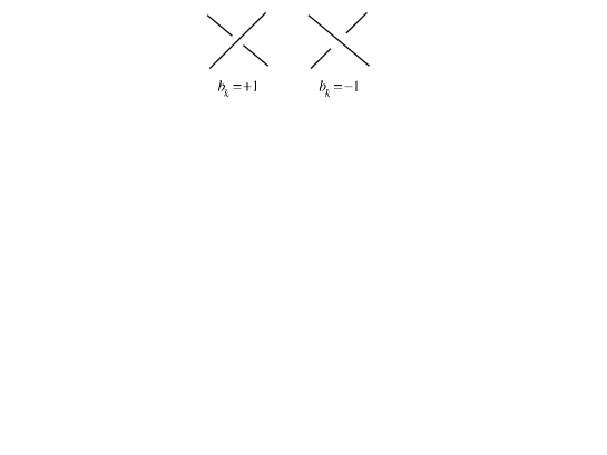
Figure 2: Definition of crossing variable for knots.

A connection to spin glasses can be made by assigning quenched random values to the crossing variables $b_{k}$, so that the links cross above and below at random. It was shown by Nechaev Nechaev:98 that in this case the Kauffman polynomial is identical, up to an irrelevant multiplicative factor, to the Potts model partition function, $Z_{\mathrm{Potts}}(q,\{J_{ij}\})=\sum_{s}\exp[-\beta H_{\mathrm{Potts}}(q,{s})]$. To explain this connection we need to introduce some terminology. The 2D-knot diagram lives on a lattice $\mathcal{M}$ composed of lines oriented at $\pm 45^{\mathrm{o}}$, intersecting at the crossings $b_{k}$, that carry the disorder. One can define a dual lattice $\mathcal{L}$, rotated by $45^{\mathrm{o}}$, so that its horizontal and vertical edges (denoted $b_{ij}$) are in one-to-one correspondence with the vertices $b_{k}$ of $\mathcal{M}$ (Fig. 6 in Nechaev:98 ). Let

$$b_{ij}=\left\{\begin{array}[]{c}-b_{k}\quad\text{{if the }}(ij)\text{-{edge is vertical}}\\ b_{k}\quad\text{{if the }}(ij)\text{-{edge is horizontal}}\end{array}\right..$$ (28)

The Potts spin states $s_{i}$ are connected to knot properties in an abstract manner; they are related to the Kauffman polynomial variable $A$, which in turn is a weight for the manner in which 2D-knot diagram is disassembled into a set of microstates (and also related to the Jones’ polynomial variable $t$: the Jones and Kauffman polynomials coincide when $t=A^{1/4}$). Precise definitions can be found in Kauffman:book ; for our purposes what matters is that the equivalence of the Kauffman polynomial to the Potts spin glass partition function is established once one assigns the Potts variables $q$ and $\beta J_{ij}$ the values

$$q = (A^{2}+A^{-2})^{2},$$

$$\beta J_{ij} = \ln(-A^{-4b_{ij}}).$$ (29)

With these identifications Nechaev has shown that the Kauffman polynomial (knot invariant) $\langle K(A)\rangle=c(A,\{b_{ij}\})Z_{\mathrm{Potts}}(q,J),$ where the constant $c$ does not depend on the spin states Nechaev:98 . Solving for $A$ we find $A=\pm[(q^{1/2}\pm(q-4)^{1/2})/2]^{1/2}$. Thus $\beta J_{ij}$ can be real only for $q\geq 4$. In the Ising spin glass case ($q=2$) we obtain a complex-valued $\beta J_{ij}$, which in turn implies complex-valued $\lambda=\tanh(\beta J)$, and hence the estimation of the QWGT polynomial with complex-valued $x$.

Finally, we note that a physically somewhat unsatisfactory aspect of the knots-Potts connection is that now the (complex-valued) temperature cannot be tuned independently from the bonds $J_{ij}$. However, this does not matter from the computational complexity perspective: we have established our third main result:

Proposition 2

Computing the Kauffman polynomial at $q=2$ is equivalent to the problem of computing the QWGT polynomial with complex-valued $x$.

Hence an efficient quantum algorithm for estimating QWGTs will be decisive for knot and graph theory as well.

VII Conclusions

The connection between QWGTs and quantum computational complexity established by KL on the one hand, and the connection between QWGTs and the spin glass and knots problems established here on the other hand, suggests that the quantum computational complexity of spin glass and knots problems may be decided via the connection to QWGTs. Similar remarks apply to a number of combinatorial problems in graph theory, via their well-established connections to knot theory. In particular, it would be desirable to find out the quantum computational complexity of questions framed in terms of properties of $S(A,\mathrm{dg}(w),\lambda,1)$, with $\lambda$ real (Ising spin glass) or complex (Kauffman polynomial with $q=2$). We leave these as open problems for future research.

Appendix A Additional Observations

A.1 The case with a Magnetic Field

A magnetic field $B$ can be included in the Hamiltonian [Eq. (1)], by adding a term $-\sum_{i\in V}B_{i}\sigma_{i}$. We can repeat the analysis above by introducing a fictitious “always-up” spin, numbered $0$. In this manner we can rewrite the magnetic field term as

$$\sum_{i\in V}B_{i}\sigma_{i}=\sum_{i\in V}B_{i0}\sigma_{i}\sigma_{0},$$ (30)

where $\sigma_{0}\equiv 1$. The corresponding graph has a “star” geometry, with spin $0$ in the center, connected to all other spins, which in turn are connected only to spin $0$ (Fig. 1c). The analysis above can then be repeated step-by-step, with the relevant subgraphs being those of the star graph. However, we then cannot recover the QWGT form, due to the extra summation over the star-graph subgraphs: Denote the latter $b^{\prime}$. Since each spin in $V$ is connected once to the central spin $\sigma_{0}$, the star graph subgraphs all have trivial parity vectors, ${\alpha}_{i}^{b^{\prime}}=1$. Then Eq. (20) is replaced by

$$\sum_{s}(-1)^{[{\alpha}^{b}+({\alpha}^{b^{\prime}})]\cdot s}=2^{|V|}\delta_{({\alpha}^{b}+{\alpha}^{b^{\prime}},0)}.$$ (31)

This causes a violation of the condition $b:Ab=0$ needed in the definition of the QWGT sum. Thus it appears that QWGTs do not include the case with a magnetic field.

A.2 Power Series Representation

Another useful representation of Eq. (23) can be obtained by grouping together all subgraphs with the same number of edges. To this end, let $b_{j}^{(k)}$ denote the $j^{\mathrm{th}}$ subgraph with $k$ edges. According to the numbering scheme introduced in Sec. II, the corresponding binary number of such a subgraph, $b_{j}^{(k)}$, is the $j^{\mathrm{th}}$ permutation of a vector of exactly $k$ 1’s and $|E|-k$ zeroes. Since $|b|$ is the Hamming weight of $b$ these subgraphs all have $|b|=k$. There are $\binom{|E|}{k}$ such subgraphs, all with equal weight $\lambda^{k}$. Therefore:

$$Z(w)={\frac{2^{|V|}}{(1-\lambda^{2})^{|E|/2}}}\times$$

$$\left(1+\sum_{k=1}^{|E|}\lambda^{k}\sum_{j=1}^{\binom{|E|}{k}}(-1)^{b_{j}^{(k)}\cdot b}\delta_{({\alpha}^{b_{j}^{(k)}},0)}\right).$$ (32)

In this form we have a series expansion in powers of $\lambda$, corresponding to the number of edges of the subgraphs.

A clear simplification results in the fully ferromagnetic Ising model ($Z_{+}$), where $w\equiv(0,0,...,0)$, and in the fully antiferromagnetic case ($Z_{-}$), where $w\equiv(1,1,..,1)$. In the latter case we have simply $b\cdot w=|b|$, so that combining the two cases we obtain from Eq. (23):

$$Z_{\pm}={\frac{2^{|V|}}{(1-\lambda^{2})^{|E|/2}}}\sum_{b}(\pm\lambda)^{|b|}\delta_{({\alpha}^{b},0)}.$$ (33)

Eq. (32), on the other hand yields:

$$Z_{\pm}={\frac{2^{|V|}}{(1-\lambda^{2})^{|E|/2}}}\left(1+\sum_{k=1}^{|E|}(\pm\lambda)^{k}\sum_{j=1}^{\binom{|E|}{k}}\delta_{({\ \alpha}^{b_{j}^{(k)}},0)}\right).$$ (34)

As already remarked, there exist an efficient classical algorithm for calculating $Z$ in the case of the fully ferromagnetic Ising model Jerrum:90 .

References

- (1) R.P. Feynman, Intl. J. Theor. Phys. 21, 467 (1982).
- (2) R.P. Feynman, Found. Phys. 16, 507 (1986).
- (3) S. Lloyd, Science 273, 1073 (1996).
- (4) D.A. Meyer, J. Stat. Phys. 85, 551 (1996).
- (5) D.A. Meyer, Phys. Rev. E 55, 5261 (1997).
- (6) B.M. Boghosian and W. Taylor, Intl. J. Mod. Phys. C 8, 705 (1997).
- (7) B.M. Boghosian and W. Taylor, Phys. Rev. E 57, 54 (1998).
- (8) S. Wiesner, Simulations of Many-Body Quantum Systems by a Quantum Computer, eprint quant-ph/9603028.
- (9) C. Zalka, Efficient Simulation of Quantum Systems by Quantum Computers, eprint quant-ph/9603026.
- (10) C. Zalka, Proc. Roy. Soc. London Ser. A 454, 313 (1998).
- (11) D.S. Abrams and S. Lloyd, Phys. Rev. Lett. 79, 2586 (1997).
- (12) G. Ortiz, J.E. Gubernatis, E. Knill, and R. Laflamme, Phys. Rev. A 64, 022319 (2001).
- (13) D.A. Lidar and H. Wang, Phys. Rev. E 59, 2429 (1999).
- (14) B.M. Terhal and D.P. DiVincenzo, Phys. Rev. A 61, 022301 (2000).
- (15) M.H. Freedman, A. Kitaev and Z. Wang, Commun. Math. Phys. 227, 587 (2002).
- (16) L.-A. Wu, M.S. Byrd, and D.A. Lidar, Phys. Rev. Lett. 89, 057904 (2002).
- (17) D.A. Lidar and O. Biham, Phys. Rev. E 56, 3661 (1997).
- (18) J. Yepez, Phys. Rev. E 63, 046702 (2001).
- (19) D.A. Meyer, Proc. Roy. Soc. London Ser. A 360, 395 (2002).
- (20) B. Georgeot and D.L. Shepelyansky, Phys. Rev. Lett. 86, 5393 (2001).
- (21) B. Georgeot and D.L. Shepelyansky, Phys. Rev. Lett. 86, 2890 (2001).
- (22) M. Terraneo, B. Georgeot, D.L. Shepelyansky, Eur. Phys. J. D 22, 127 (2003).
- (23) C. Zalka, Comment on “Stable Quantum Computation of Unstable Classical Chaos”, eprint quant-ph/0110019.
- (24) L.H. Kauffman, Quantum Computing and the Jones Polynomial, eprint math.QA/0105255.
- (25) L. Kauffman, Knots and Physics, Vol. 1 of Knots and Everything (World Scientific, Singapore, 2001).
- (26) L. Onsager, Phys. Rev. 65, 117 (1944).
- (27) R.J. Baxter, Exactly Solved Models in Statistical Mechanics (Academic, New York, 1982).
- (28) H.S. Green and C.A. Hurst, Order-Disorder Phenomena (Interscience Publishers, London, 1964).
- (29) E. Ising, Z. der Physik 31, 253 (1925).
- (30) M.R. Jerrum, A. Sinclair, Proc. 17th ICALP, EATCS 462 (1990).
- (31) R.H Swendsen and J.-S. Wang, Phys. Rev. Lett. 58, 86 (1987).
- (32) A. Nayak, L. Schulman, and U. Vazirani, manuscript, unpublished.
- (33) D. Randall and D.B. Wilson, in Sampling spin configurations of an Ising system (1999), p. S959, 10th Symposium on Discrete Algorithms (SODA).
- (34) E. Knill and R. Laflamme, Inf. Proc. Lett. 79, 173 (2001).
- (35) V.F.R. Jones, Pacific J. Math. 137, 311 (1989).
- (36) V.F.R. Jones, Bull. Amer. Math. Soc. 12, 103 (1985).
- (37) F. Jaeger, D. Vertigen, D. Welsh, Math. Proc. Cambridge Philos. Soc. 108, 35 (1990).
- (38) M.H. Freedman, A. Kitaev, M.J. Larsen, and Z. Wang, Topological Quantum Computation, eprint quant-ph/0101025.
- (39) L.H. Kauffman and S.J. Lomonaco, New J. Phys. 4, 73.1 (2002).
- (40) C.H. Papadimitriou, Computational Complexity (Addison Wesley Longman, Reading, Massachusetts, 1995).
- (41) R.J. Wilson, Introduction to Graph Theory, 4 ed. (Addison-Wesley, Reading, Massachusetts, 1997).
- (42) D. Aharonov, Annual Reviews of Computational Physics VI (2000).
- (43) Scott Aaronson’s “complexity zoo” page, http://www.cs.berkeley.edu/~aaronson/zoo.html.
- (44) L. Adleman, J. DeMarris, and M. Huang, SIAM J. on Computing 26, 1524 (1997).
- (45) D.L. Vertigan, J. Combin. Theory A 220, 53 (1992).
- (46) N. Alon, A.M. Frieze, D. Welsh, Electronic Colloquium on Computational Complexity 1(5) (1994).
- (47) L.H. Kauffman, Topology 26, 395 (1987).
- (48) S. Nechaev, Statistics of knots and entangled random walks, eprint cond-mat/9812205.