Tailoring photonic entanglement in high-dimensional Hilbert spaces

Abstract

We present an experiment where two photonic systems of arbitrary dimensions can be entangled. The method is based on spontaneous parametric down conversion with trains of $d$ pump pulses with a fixed phase relation, generated by a mode-locked laser. This leads to a photon pair created in a coherent superposition of $d$ discrete emission times, given by the successive laser pulses. Entanglement is shown by performing a two-photon interference experiment and by observing the visibility of the interference fringes increasing as a function of the dimension $d$. Factors limiting the visibility, such as the presence of multiple pairs in one train, are discussed.

Entanglement is one of the essential features of quantum physics. It leads to non classical correlation between different particles. Entanglement of two-levels systems (qubits) has been extensively studied, both theoretically and experimentally, in order to perform fundamental tests of quantum mechanics and to implement a number of protocols proposed in the burgeoning field of quantum information science (see e.g. tittel01 for a recent review). However, it is interesting to explore higher-dimensional Hilbert spaces. From a fundamental point of view, increasing the complexity of the systems and the dimension of the Hilbert space might lead to a further insight into the subtleties of quantum physics. For instance, high-dimensional entangled states give experimental predictions which differ more radically from classical physics Kaszlikowski00 ; collins02 than entangled qubits. They could also decrease the quantum efficiency required to close the detection loophole in Bell experiments massar01 . In the more applied context of quantum information science, high dimensional entangled states might also be of interest. In particular, high-dimensional systems can carry more information than two-dimensional systems and increase the noise threshold that quantum key distribution protocols can tolerate hbp2000 ; cerf01 . Moreover, using entangled qudits might increase the efficiency of Bell state measurements for quantum teleportation Witthaut03 . Finally, although most of the proposed protocols require only entangled qubits, some protocols involving qutrits (3-dimensional systems) have been recently proposed, such as the Byzantine agreement fitzi01 and quantum coin tossing coin .

Only recently the first experiments started to explore entanglement in higher dimensions. Two directions can be considered. First, one can take profit of multi-photon entanglement, as obtained for example in higher order parametric down conversion Lamas01 ; Howell02 . Second, one can use the entanglement of two high-dimensional systems. Entanglement of orbital angular momentum of photons has been for instance proposed and demonstrated in this context Mair01 ; Vaziri02 . Energy-time entanglement has also been recently analyzed in 3 dimensions thew03Q , using unbalanced 3-arm fiber optic interferometers in a scheme analogous to the Franson interferometric arrangement for qubits.

All these methods so far have been demonstrated only for qutrits and it will be difficult to implement them in higher dimensions. In contrast, we recently proposed a simple method to entangle two photonic systems of arbitrary dimensions. It is based on spontaneous parametric down-conversion (SPDC) with a sequence of pump pulses with a fixed phase relation generated by a mode-locked laser, leading to high-dimensional time-bin entanglement HdR02 . In this paper, we report on an experimental realization of this scheme, where it is possible to choose arbitrarily the dimension of the entangled photons Hilbert space. An advantage of our scheme is that it enables the generation of entangled states in arbitrary dimensions in a scalable way with only two photons note0 . We perform a simple analysis which is sufficient to show entanglement, although it does not provide a full information about the states.

Before describing the experiment, let us recall the basics of high-dimensional time-bin entanglement. Suppose a SPDC process with a train of $d$ pump pulses with a fixed phase relation. Providing that the probability of creating more than one pair in $d$ pulses is negligible and excluding the vacuum, the state after SPDC is HdR02 :

$$|\Psi\rangle_{PDC}=\sum_{j=1}^{d}c_{j}e^{i\phi_{j}}|j,j\rangle$$ (1)

where $|j,j\rangle\equiv|j_{A},j_{B}\rangle$ corresponds to a photon pair created by the pulse (or time-bin) j, with relative amplitude $c_{j}$ and phase $\phi_{j}$. The phase reference $\phi_{1}$ is set at 0. $A$ and $B$ are the two SPDC modes, $d$ is an integer that can be arbitrarily large and $\sum_{j=1}^{d}c_{j}^{2}=1$.

This method enables to create any bipartite high-dimensional state. By selecting the number of pump pulses we can choose the dimension of the entangled photons Hilbert space. In our experiment we construct trains of $d$ pulses, where $d$ can be varied from 1 to 20, with constant amplitudes $c_{j}$ and with constant phase shifts $\phi_{j}-\phi_{j-1}=\phi=cst.$ Note that by inserting a phase and/or amplitude modulator before the down-converter, we could in principle modulate their amplitudes and phases, thus varying the coefficients $c_{j}$ and $\phi_{j}$ in order to generate arbitrary non-maximally entangled states.

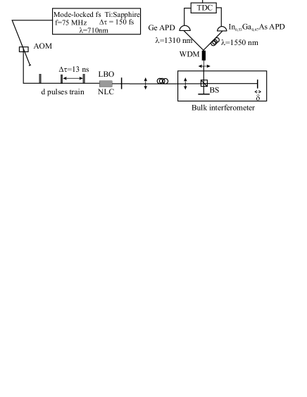
Figure 1: Schematic of the experiment. See text for details.

A complete analysis of such high dimensional entangled states would require the use of d-arm interferometers, such that the amplitudes and phases of all time-bins can be probed. An alternative could be given by the use of fiber loops or Fabry-Perot interferometers, as proposed in HdR02 . Here, we used a 2-arm interferometer, which already shows high-dimensional entanglement. The travel time difference between the long and the short arm of this interferometer is equal to the time between 2 pump pulses $\Delta\tau$ (see Fig. 1). This means that a photon travelling through the short arm will remain in the same time-bin while a photon travelling through the long arm will move to the next time-bin. We restrict ourself to the events where both photons of one pair travel the same path in the interferometer, and are thus detected with a time difference $\Delta t=t_{A}-t_{B}=0$. In this case, the evolution of the state of Eq.(1) in the interferometer can be written as (not normalized):

$$\left|\Psi_{int}\right\rangle = \left|1,1\right\rangle+\sum_{j=2}^{d}\left|j,j\right\rangle(e^{\phi_{j}}+e^{i(\delta_{A}+\delta_{B}+\phi_{j-1})})$$ (2)

$$+ e^{i(\delta_{A}+\delta_{B}+\phi_{d})}\left|d+1,d+1\right\rangle$$

where $\delta_{A,B}$ are the phases introduced in the long arm of the interferometer for the photons $A$ and $B$ and with $\phi_{1}=0$. We see that for all time-bins except the first and the last one we have a superposition of two indistinguishable processes. If we record all the processes leading to a coincidence with $\Delta t=0$, i.e if we don’t postselect the interfering terms, the coincidence count rate varies as

$$R_{c}\sim 1+V_{d}\cos(\delta_{A}+\delta_{B}-\phi)$$ (3)

where $\phi_{j}-\phi_{j-1}=\phi$ for all $j$. From the $2d$ different processes, two are always completely distinguishable (the first and the last time bin). Therefore, the maximal visibility of the interference fringes, $V_{d}$, depends on the dimension $d$ as:

$$V_{d}=V_{max}\frac{d-1}{d}$$ (4)

where $V_{max}$ is the maximum visibility due to experimental imperfections. This analysis is valid if the phase difference between 2 pulses is constant, which is the case in a mode-locked laser. Two contributions might affect the stability. First the laser cavity length may vary slowly due to thermal drift. This drift has been measured ($\sim 2\mu m$ per hour) and is negligible in the time-scale of a round trip time. Second, one could imagine faster fluctuations of the optical cavity length due e.g. to mechanical vibrations. This seems however unlikely, since important fluctuations would destroy the laser operation. To further confirm this point, we make the following reasoning. If we consider a small phase noise between 2 consecutive pulses with a Gaussian distribution of width $\delta\epsilon$, the visibility will be reduced to: $V=V_{d}\exp(-\frac{1}{2}\delta\epsilon^{2})$. The phase noise between pulse j and pulse j+m also has a gaussian distribution of width $\sqrt{m}\delta\epsilon$, leading to a visibility $V=V_{d}\exp(-\frac{1}{2}(m)\delta\epsilon^{2})$. Observing a visibility $V_{d}$ close to optimal is thus a confirmation that the phase noise $\delta\epsilon\ll\pi$ and consequently that the coherence is maintained over many time bins.

In our experiment, we use trains of $d$ pump pulses, where $d$ can be varied from 1 to 20, and we observe the visibility of the two photon interference as a function of the dimension $d$. A schematic of the experiment is presented in Fig. 1. The pump laser is a Ti-Sapphire femtosecond mode-locked laser producing 150fs pulses at a wavelength of 710 nm. The time between 2 pulses is $\Delta\tau$ = 13 ns. To construct the pulse trains, the pump beam is focussed into a 380MHz acousto-optic modulator (AOM, from Brimrose) which reflects the incoming beam with an efficiency of $\approx 50\%$ when it is activated. This activation can be triggered externally, with a TTL signal of variable width synchronized with the laser pulses. The rise time is around 6ns. The width of this signal thus determines the number of pulses per train. The reflected beam containing the pulse trains is then used to pump a non-linear Lithium triborate (LBO) crystal. Non degenerate photon pairs at 1310/1550 nm wavelength are created by SPDC and then sent to the analyzer, which is a two-arm bulk Michelson interferometer, where the long arm introduces a delay $\Delta\tau$=13 ns with respect to the short one, corresponding to a physical path-length difference of 1.95 m note1 . The pump power is kept low, in order to keep the probability of having more than one pair per train small. Photons exiting one output of the interferometer together are first focussed into an optical fiber and then separated with a wavelength division multiplexer (WDM). The 1310 nm photon is detected by a passively quenched LN2 cooled Ge Avalanche Photo Diode (APD, from NEC), with a quantum efficiency $\eta$ of around 10$\%$ for 40kHz of dark counts. The 1550 nm photon is detected with an InGaAs photon counting module (from idQuantique), featuring a quantum efficiency of around 30$\%$ for a dark count probability of $10^{-4}$ per ns and operating in gated mode. The trigger is given by a coincidence between the Ge APD and a 1-ns signal delivered simultaneously with each laser pulse ($t_{0}$), in order to reduce the accidental coincidences. The signals from the APDs are finally sent to a time-to-digital converter, in order to record the photons arrival time histogram. A small coincidence window of around 1 ns is selected around the interfering peak (i.e the peak with $\Delta t=0$).

If we record the coincidence count rate as a function of the phase shift in the interferometer, we obtain sinusoidal curves with a visibility increasing with the dimension $d$ (see Fig.2). Net visibilities (i.e with accidental coincidence count rate subtracted) as a function of the dimension $d$ are plotted in Fig.3. The solid line is a fit using Eq. (4). The good agreement between experimental data and theory confirms that the dimension of the entangled photons is given by the number of pump pulses d. We find a maximal visibility of $91.6\pm 1.2\%$.

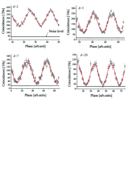
Figure 2: Two-photon interference visibility for different dimensions d. The solid line is a sinusoidal fit from which we can deduce the net visibility of the fringes. The level of accidental coincidence is indicated by the straight line.

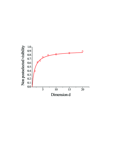
Figure 3: Two-photon interference visibility as a function of the dimension of the Hilbert space. The black circles are experimental points. The solid line is a fit with eq. 4

.

We now discuss the factors limiting the visibility which, as we will see, is not reduced by a possible phase noise between pump pulses. A first factor is the possible creation of more than one pair per pulse train. The spectral bandwidth of the (not filtered) created photons is about 100nm, corresponding to a coherence time of $\approx 25fs$, much smaller than the duration of the pump pulse. In this limit, any $2n$ photons state can be described as $n$ independent pairs. The probability of producing $n$ pairs in a given pulse is distributed according to the Poissonian distribution of mean value $\mu$: $p_{n}=e^{-\mu}\,\frac{\mu^{n}}{n!}.$ The starting point for the calculation of the loss of visibility due to multiple pairs is the fact that the total coincidence count rate can be written

$$R = R_{1}\,(1+V_{d}\cos\theta)\,+\,R_{2}\,.$$ (5)

The first term of the sum means that, for each pair created, the two-photon process described above can take place, leading to an interference fringe of visibility $V_{d}$. The additional rate $R_{2}$ is what comes from the multi-pair pulses, when one detects coincidence of photons belonging to independent pairs. In our case there are only two kinds of contributions to $R_{2}$: either the photons were created in the same time-bin ($R_{2,s}$), or in consecutive time-bins ($R_{2,c}$); if the independent pairs are created in more distant time-bins, no coincidence is registered.

Now, we calculate $R_{1}$, $R_{2,s}$ and $R_{2,c}$ explicitly. $R_{1}$ is proportional to the mean number of pairs created $\mu d$. The factor of proportionality is given by the probability that a photon pair leads to a coincident detection (i.e with $\Delta t=0$), which is $\frac{1}{2}$ note2 . Hence finally $R_{1}=\frac{1}{2}\,\mu\,d$. Let us now calculate $R_{2,s}$. With $n$ pairs in a given time-bin, one can create $\frac{n(n-1)}{2}$ couples, so the mean number of such couples in d time-bins is $d\sum_{n}p_{n}\frac{n(n-1)}{2}=d\frac{\mu^{2}}{2}$. By inserting the probability of coincidence note4 , we find: $R_{2,s}=\frac{\mu^{2}}{2}\,d\,.$ Let us finally calculate $R_{2,c}$. If $n_{k}$ is the number of pairs in time-bin $k$, the number of pairs in consecutive time-bins is $m=n_{1}\times n_{2}+n_{2}\times n_{3}+...+n_{d-1}\times n_{d}$. The average of the random variable $m$ is $\langle m\rangle=\sum_{n_{1}}...\sum_{n_{d}}p_{n_{1}}...p_{n_{d}}\,m(n_{1},...,n_{d})\,=\,(d-1)\,\mu^{2}\,$. In this case, only half of the processes lead to a coincident detection. We thus obtain $R_{2,c}=\frac{1}{2}\,\mu^{2}\,(d-1)\,$. Inserting these results into (5) we find $R\,\propto\,1+V(\mu,d)\cos\theta$ with

$$V(\mu,d) = V_{d}\,\frac{1}{1+2\mu-\mu/d}\,.$$ (6)

To validate our model, we measured the visibility as a function of $\mu$, for $d$=20 (see Fig. 4). The factor $\mu$, which is proportional to the pump power is determined by the side peak method, explained in detail in marcikic02 . The solid line is a fit of Eq.(6), in good agreement with the experimental data.

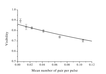
Figure 4: Visibility of the interference fringes as function of the mean number of pairs per pulse $\mu$, for d=20.

For the measurement of Fig. 3 (not corrected), $\mu$ is kept low ($<0.025$) so that we estimate the maximal visibility due to multiple pairs to $(97\pm 1)\%$.

Another factor that affects the visibility is the non perfect alignment of the analyzing interferometer. Ideally, the transmission in the long and the short arm should be the same for both wavelength. Due to the fact that the interferometer is long and that the two photons have different wavelengths, obtaining a good alignment is very difficult. To calculate the influence of a misalignment we write $t_{s}$ and $t_{l}$ the transmission probability amplitudes for the short and the long arm respectively. For simplicity, we assume them to be the same for both wavelengths. In this case the coincidence count rate (if we take only the interfering terms) is $R_{c}\sim t_{s}^{4}+t_{l}^{4}+2t_{s}^{2}t_{l}^{2}\cos(\delta_{A}+\delta_{B}-\phi)$, leading to a visibility:

$$V=\frac{2t_{s}^{2}t_{l}^{2}}{t_{s}^{4}+t_{l}^{4}}$$ (7)

In our experiment, we typically obtain transmission differences between the long and the short arm between 1 and 1.5 dB, which limit the maximal visibility to around $(96\pm 1)\%$. Moreover, the states we create are not completely maximally entangled, due to the fact that the first and the last pump pulses in a train have a slightly smaller intensity. Finally, the interferometer might not have a perfect visibility. To take into account these last factors, we estimate a maximal visibility of $(99\pm 1)\%$.

Considering all the above mentioned factors, we find an optimal visibility of $(92.2\pm 1.6)\%$ which fits with the measured value of $(91.6\pm 1.2)\%$. This is a confirmation that the phase noise is negligible and consequently that the coherence is kept over many time-bins and that we generate entangled qudits.

In conclusion, we reported an experiment where we entangled two photonic systems of arbitrary discrete dimensions. The simple analysis presented in this paper already allows us to demonstrate the creation of a photon pair in a coherent superposition of $d$ emission times, providing evidence of high-dimensional entanglement. More complex analysis with d-arm interferometers should allow to reveal all the quantum information content of such states (e.g. nonlocality).

The authors would like to thank Claudio Barreiro and Jean-Daniel Gautier for technical support. Financial support by the Swiss NCCR Quantum Photonics, and by the European project RamboQ is acknowledged.

References

- (1) W. Tittel and G. Weihs, Quant. Inf. Comput. 1, 3-56 (2001)
- (2) D. Kaszlikowski et al, Phys. Rev. Lett. 85, 4418 (2000)
- (3) D. Collins et al, Phys. Rev. Lett. 88, 040404 (2002)
- (4) S. Massar, Phys. Rev. A 65, 032121 (2002)
- (5) H. Bechmann-Pasquinucci and W. Tittel, Phys. Rev. A 61, 062308 (2000)
- (6) N. J. Cerf et al, Phys. Rev. Lett. 88, 127902 (2002)
- (7) D. Witthaut, M. Fleischhauer, quant-ph/0307140
- (8) M. Fitzi, N. Gisin, and U. Maurer, Phys. Rev. Lett. 87, 217901 (2001)
- (9) A. Ambainis, Proc. STOC 01, 134 (2001).
- (10) A. Lamas-Linares, J.C.Howell and D.Bouwmeester, Nature, 412 887-890 (2001)
- (11) J. C. Howell, A. Lamas-Linares, and D. Bouwmeester , Phys. Rev. Lett. 88, 030401 (2002)
- (12) A. Mair et al, Nature 412, 313 - 316 ( 2001)
- (13) A. Vaziri, G. Weihs, and A.Zeilinger Phys. Rev. Lett. 89, 240401 (2002)
- (14) R.T.Thew et al, quant-ph/0307122(2003)
- (15) H.de Riedmatten et al, Quant.Inf.Comput 2,425-433 (2002)
- (16) This is an advantage compared to the multiphoton schemes since the detection efficiency remains constant for any dimension.
- (17) The time difference between 2 pump pulses can be determined very precisely by measuring the repetition rate of the laser. This allows us to determine the path length difference of the interferometer with a precision better than the pump coherence length (i.e a few tens of microns)
- (18) Each photon can follow two paths note3 : long () or short() arm of the interferometer, so there are 4 different paths for the pair. Only two of them ( and ) lead to a coincident detection.
- (19) We restrict ourself to the case where both photons exit the same output of the interferometer. We omit to write a global factor , where is the transmission in the interferometer and the quantum efficiency of the detectors. But we take into account that when calculating :if a given ”path” leads to several coincident detection, we add the probabilities for each process.
- (20) Independently on how many pairs were present, we focus on the two pairs that gave each one photon for the detection. The considered event may have happened for these paths: , , and , where the left part corresponds to the first pair and the right part to the second one, and . Altogether, this gives 16 possible paths note3 , and the total number of paths for four photons is .
- (21) I. Marcikic et al Phys. Rev. A 66, 062308 (2002)