Optical telecom networks as weak quantum measurements with post-selection

1 Introduction

In this work we establish a link between two apparently unrelated subjects: polarization effects in optical fibers and devices, and the quantum theory of weak measurements [1]. We show that the abstract concept of weak measurements followed by post-selection, introduced a decade ago by quantum theorists, naturally appears in the everyday physics of telecom networks.

Our analogy works as follows. First, polarization mode dispersion (PMD) [2] performs polarization measurements by spatially separating the fiber’s eigenmodes. It turns out that the usual telecom limit for PMD, where dispersion has to be minimized, corresponds to the quantum regime of weak measurements. Then polarization dependent losses (PDL) [2] perform post-selection in a very natural way: one post-selects those photons that have not been lost. This is non-trivial physics since the losses depend precisely on the measured degree of freedom: the polarization of light. In case of an infinite PDL (i.e. a polarizer) the post-selection is done on a pure state. For a finite PDL, the post-selection is done on a mixed state. Thus the amount of PDL characterizes the kind of post-selection involved.

We show also that the quantum formalism of weak measurements can simplify some ”telecom” calculations and gives a better understanding of the physics of networks. A telecom network can be described as a concatenation of elements with PMD (fibers) and some with PDL (couplers, isolators, etc). A simple formula for the mean time-of-arrival for an arbitrary concatenation of PMD and PDL elements is derived.

2 Polarization mode dispersion

Polarization mode dispersion (PMD) is the most important polarization effect in optical fibers. It is due to the birefringence of the fiber. In standard optics, a fiber is represented by a channel supporting two polarization modes. The main consequence of PMD, is that the time of flight along the fiber will be different for each mode.

Before going into calculations we would like to clarify the notations. We use the formalism of two dimensional Jones vectors to describe polarization. In this representation a classical state of polarization is equivalent to a quantum spin $\frac{1}{2}$. The three typical pairs of polarizations - horizontal-vertical linear, diagonal linear, left-right circular - are described respectively by the eigenvectors of the Pauli matrices

$$\sigma_{x}=\left(\begin{array}[]{cc}0&1\\ 1&0\end{array}\right)\quad\sigma_{y}=\left(\begin{array}[]{cc}0&-i\\ i&0\end{array}\right)\quad\sigma_{z}=\left(\begin{array}[]{cc}1&0\\ 0&-1\end{array}\right)\,.$$ (7)

We mostly use the eigenstates of $\sigma_{z}$

$$\sigma_{z}\mbox{$|H\rangle$}=\mbox{$|H\rangle$}\quad\mbox{and}\quad\sigma_{z}\mbox{$|V\rangle$}=-\mbox{$|V\rangle$}$$ (8)

A general pure state of polarization is a complex superposition of these two states. The state $\mbox{$|+\hat{n}\rangle$}=\cos(\theta/2)\mbox{$|H\rangle$}+\sin(\theta/2)e^{i\varphi}\mbox{$|V\rangle$}$ corresponds to the point $\hat{n}=(\theta,\varphi)$ on the Poincaré sphere.

Let’s consider a PMD fiber of length $L$ with birefringence vector $\vec{\xi}$. We define the fiber’s axis to be the $z$ direction. So $|H\rangle$ and $|V\rangle$, the eigenstates of $\sigma_{z}$, are the eigenmodes of the fiber. We consider a polarized gaussian pulse with coherence time $t_{c}$. This pulse can be thought of as a classical light pulse or as a quantum single photon non-monochromatic state. Taking into account both energy and polarization degrees of freedom, the complete initial state reads

$$\mbox{$|\Psi_{in}\rangle$}\,=\frac{1}{(t_{c}\sqrt{2\pi})^{1/2}}\,e^{-t^{2}/4t_{c}^{2}}\,\otimes\,\big{(}\alpha\mbox{$|H\rangle$}+\beta\mbox{$|V\rangle$}\big{)}\,\equiv\,g(t)\otimes\mbox{$|\psi_{0}\rangle$}\,,$$ (9)

where $\alpha,\beta$ are complex numbers and satisfy $|\alpha|^{2}+|\beta|^{2}=1$. In this equation, as usual, the gaussian function $g(t)$ is normalized so that

$$G(t)\,\equiv\,g(t)^{2}=\frac{1}{t_{c}\sqrt{2\pi}}\,e^{-t^{2}/2t_{c}^{2}}$$ (10)

is a probability distribution. Our coordinate system $t$ corresponds to the time-of-arrival of the pulse and travels at the speed of light in the fiber (without PMD) $v_{f}=c/n$, where $n$ is the refractive index in the fiber. A pulse centered at $t=0$ propagates at speed $v_{f}$.

PMD is a unitary operation represented by the operator

$$U(\xi,\hat{z})=e^{i\frac{\xi}{2}\omega\sigma_{z}}=\cos(\frac{\xi\omega}{2})\leavevmode\hbox{\small 1\normalsize\kern-3.30002pt1}+i\sin(\frac{\xi\omega}{2})\sigma_{z}\,\,.$$ (11)

where $\xi=\,\parallel\vec{\xi}\parallel$. To compute the evolution for each eigenmode of the fiber, we have to Fourier-transform the input state $g(t)\otimes\mbox{$|H,V\rangle$}$ into the frequency domain, apply the PMD operator to any monochromatic component, and integrate back to the time domain. Note that by $|H,V\rangle$, we mean $|H\rangle$ or $|V\rangle$. Thus we have

$$U(\xi,\hat{z})\,g(t)\otimes\mbox{$|H,V\rangle$}=\int d\omega\tilde{g}(\omega)e^{-i\omega t}\,e^{i\frac{\xi}{2}\omega\sigma_{z}}\,\mbox{$|H,V\rangle$}$$ (12)

where $\tilde{g}(\omega)$ is the Fourier-transform of $g(t)$. Since our gaussian pulse is centered in frequency $\omega_{0}$ we apply the following change of coordinate $\omega\rightarrow\omega-\omega_{0}$. We have

$$U(\xi,\hat{z})\,g(t)\otimes\mbox{$|H,V\rangle$} = \int d\omega\tilde{g}(\omega-\omega_{0})e^{-i(\omega-\omega_{0})t}\,e^{i\frac{\xi}{2}\omega\sigma_{z}}\,\mbox{$|H,V\rangle$}$$ (13)

$$= \int d\omega\tilde{g}(\omega-\omega_{0})e^{-i(\omega-\omega_{0})(t\mp\frac{\xi}{2})}\,e^{\pm i\frac{\xi}{2}\omega_{0}}\,\mbox{$|H,V\rangle$}$$

$$= g(t\mp\frac{\xi}{2})\,\otimes\,e^{\pm i\frac{\xi}{2}\omega_{0}}\,\mbox{$|H,V\rangle$}\,\,.$$

The above equation shows that the mean time of arrival for each eigenmode is shifted by the same quantity ($\xi/2$) in either direction. Usually the time separating the mean time-of-arrival of the two modes is called the differential group delay (DGD) and noted $\delta\tau$ . Thus the output state reads

$$\mbox{$|\Psi_{PMD}\rangle$}=\tilde{\alpha}g_{-}(t)\mbox{$|H\rangle$}+\tilde{\beta}g_{+}(t)\mbox{$|V\rangle$}\,,$$ (14)

where we have omitted the tensor products and defined

$$\tilde{\alpha}\equiv e^{i\frac{\delta\tau}{2}\omega_{0}}\alpha\quad,\quad\tilde{\beta}\equiv e^{-i\frac{\delta\tau}{2}\omega_{0}}\beta\quad,\quad g_{\pm}(t)\equiv g(t\pm\frac{\delta\tau}{2})\,\,.$$ (15)

So the effect of PMD is a spatial separation of the fiber’s eigenmodes $|H\rangle$ and $|V\rangle$ combined with a rotation of the polarization around the $z$ axis. This global phase is irrelevant for the link we want to establish and will therefore always be absorbed in the polarization state

$$\mbox{$|\psi\rangle$}\equiv e^{i\omega_{0}\frac{\delta\tau}{2}\sigma_{z}}\mbox{$|\psi_{0}\rangle$}=\tilde{\alpha}\mbox{$|H\rangle$}+\tilde{\beta}\mbox{$|V\rangle$}\,\,.$$ (16)

Note that $|H\rangle$ and $|V\rangle$ are respectively the fastest and slowest polarization modes in the fiber.

The measurement analogy now goes like this. Different polarization modes will arrive at different times. Thus by measuring the mean time-of-arrival of a pulse one can obtain some information about its state of polarization. Depending on whether the delay between the two polarization modes is large (small) compared to the coherence time of the pulse, the measurement of polarization achieved by PMD is strong (weak) (see Fig. 1). In telecom optics the interesting limit is always the second one since dispersion has to be minimized.

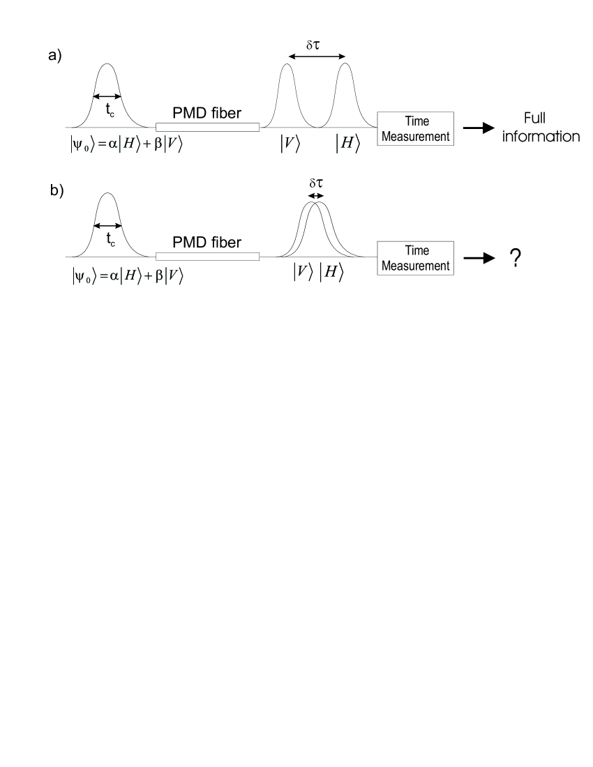
Figure 1: PMD as a polarization measuring device. a) the measurement is strong: the time-of-arrival gives full information about the polarization of the pulse. b) the measurement is weak: no discrimination possible.

In standard quantum mechanics, a measurement is an interaction between two systems: the physical system to be measured and the measuring device, usually called a pointer [5]. The change in the position of the pointer, due to the measurement, provides some information about the state of the measured system. In our case the energy degree of freedom of the pulse plays the role of the pointer, while the polarization is the measured system. Thus pointer and measured system are here different degrees of freedom of the same physical system. PMD provides the necessary interaction between the pointer and the measured system since energy and polarization degrees of freedom are entangled in the output state (14). However, PMD alone, without the final measurement of the time-of-arrival, is not a measurement since it is a reversible operation.

3 Polarizer: post-selection on a pure state

3.1 Strong measurement

Our aim is to describe networks. A network is an arbitrary concatenation of PMD and PDL elements. In this section we study the simplest one: a PMD fiber followed by an element with infinite PDL, i.e. a polarizer. Note that this setup corresponds to the usual scenario in which weak measurements are studied, since the system is pre- and post-selected. Here the post-selection is done on a pure state, since the polarizer projects onto a linear polarization

$$\mbox{$|\phi\rangle$}=\mu\mbox{$|H\rangle$}+\nu\mbox{$|V\rangle$}\,.$$

At the output, we measure the time-of-arrival. So, the final state is

$$\mbox{$|\Psi_{out}\rangle$}=\mbox{$|\phi\rangle$}\mbox{$\langle\phi|\Psi_{PMD}\rangle$}=\Big{[}\tilde{\alpha}\bar{\mu}\,g_{-}(t)+\tilde{\beta}\bar{\nu}\,g_{+}(t)\Big{]}\otimes\mbox{$|\phi\rangle$}\,\equiv\,F(t)\otimes\mbox{$|\phi\rangle$}\,.$$ (17)

Note that $|F(t)|^{2}$ must be normalized in order to be a probability distribution. As we have seen above, because of PMD some information about the preparation is contained in the shape, $F(t)$, of the output pulse.

When $\delta\tau>>t_{c}$ the two gaussians do not overlap, $g_{-}(t)g_{+}(t)\approx 0$, and it is possible to discriminate between the two polarization eigenmodes. The detected intensity corresponds to two well-separated gaussians. From (17) we have

$$I(t)\,\equiv\,|F(t)|^{2} = |\tilde{\alpha}\bar{\mu}|^{2}\,G_{-}(t)\,+\,|\tilde{\beta}\bar{\nu}|^{2}\,G_{+}(t)\,=$$ (18)

$$= \mbox{Prob}(\phi|H)\mbox{Prob}(H|\psi)\,G_{-}(t)\,+\,\mbox{Prob}(\phi|V)\mbox{Prob}(V|\psi)\,G_{-}(t)$$

where we have introduced obvious notations like $\mbox{Prob}(H|\psi)=|\tilde{\alpha}|^{2}$ etc. The probability that the polarization was $|H\rangle$, given the preparation and the post-selection, is, in the limit $\delta\tau>>t_{c}$

$$\mbox{Prob}(H) = \frac{\int_{0}^{\infty}I(z)dz}{\int_{-\infty}^{\infty}I(z)dz}\,=\,\frac{\mbox{Prob}(\phi|H)\mbox{Prob}(H|\psi)}{\sum_{K=H,V}\mbox{Prob}(\phi|K)\mbox{Prob}(K|\psi)}\,.$$ (19)

This is exactly the Aharonov-Bergmann-Lebowitz (ABL) rule, which is in fact the classical rule for the probability of sequential events. Of course, $\mbox{Prob}(V)=1-\mbox{Prob}(H)$. One can also compute the mean time of arrival

$$\langle t\rangle=\mbox{Prob}(H)\frac{\delta\tau}{2}+\mbox{Prob}(V)\big{(}-\frac{\delta\tau}{2}\big{)}\,.$$ (20)

Since the mean value of $\sigma_{z}$ is simply $\langle\sigma_{z}\rangle=\mbox{Prob}(H)-\mbox{Prob}(V)$, we have

$$\langle t\rangle\,=\,\frac{\delta\tau}{2}\,\langle\sigma_{z}\rangle\,.$$ (21)

The interpretation of equation (21) is a key point of our work and needs to be carefully explained. In quantum-mechanical terms, $\sigma_{z}$ is the observable that is measured by the time delay $\delta\tau$, and (21) shows that its mean value is associated to the mean time-of-arrival $\langle t\rangle$ in the case of a strong measurement. What happens now when the measurement is weakened? The point is that, in contrast to $\mbox{Prob}(H)$ and $\mbox{Prob}(V)$, the mean time-of-arrival is a physical quantity that can be defined and measured in any situation (for a strong or weak measurement, with or without post-selection). We admit that (21) is the definition of the mean value of $\sigma_{z}$ when measured by introducing a time delay $\delta\tau$ between $|H\rangle$ and $|V\rangle$.

3.2 General measurement

We can now remove all assumptions on the strength of the measurement and derive an analytical formula for the mean time-of-arrival $\langle t\rangle$. Lets consider again the output state (17). Without any assumption on the gaussians, the intensity is now

$$I(t)\,\equiv\,|F(t)|^{2}=|A|^{2}\,G_{-}(t)\,+\,|B|^{2}\,G_{+}(t)+2Re(\bar{A}B)g_{-}(t)\,g_{+}(t)\,,$$ (22)

where $A\equiv\tilde{\alpha}\bar{\mu}$ and $B\equiv\tilde{\beta}\bar{\nu}$. The mean time-of-arrival is given by

$$\langle t\rangle=\frac{\int_{-\infty}^{\infty}tI(t)dt}{\int_{-\infty}^{\infty}I(t)dt}=\frac{(|A|^{2}-|B|^{2})\frac{\delta\tau}{2}}{|A|^{2}+|B|^{2}+2Re(\bar{A}B)\int_{-\infty}^{\infty}g_{-}(t)\,g_{+}(t)dt}\,.$$ (23)

We evaluate separately the remaining integral

$$\int_{-\infty}^{\infty}g_{-}(t)\,g_{+}(t)\,dt=e^{-\frac{1}{2}({\delta\tau}/{2t_{c}})^{2}}\underbrace{\frac{1}{t_{c}\sqrt{2\pi}}\int_{-\infty}^{\infty}e^{-{t^{2}}/{2t_{c}^{2}}}\,dt}_{=1}=e^{-\frac{1}{2}({\delta\tau}/{2t_{c}})^{2}}\,.$$ (24)

So finally we find

$$\langle t\rangle=\frac{\delta\tau}{2}\,\frac{(|A|^{2}-|B|^{2})}{|A|^{2}+|B|^{2}+2Re(\bar{A}B)\,e^{-\frac{1}{2}({\delta\tau}/{2t_{c}})^{2}}}\,.$$ (25)

An important feature of equation (25) is that the dependance in the strength of the measurement (i.e. in $\delta\tau/t_{c}$) is very explicit. Of course in the limit $\delta\tau/t_{c}\rightarrow\infty$, corresponding to a strong measurement our previous result is recovered.

Since equation (25) is completely general we can compute the mean time-of-arrival in the case of a weak measurement, corresponding to the telecom limit of PMD. When $\delta\tau<<t_{c}$ equation (25) becomes

$$\ \langle t\rangle=\frac{\delta\tau}{2}\,\frac{(|A|^{2}-|B|^{2})}{|A|^{2}+|B|^{2}+2Re(\overline{A}B)}=\frac{\delta\tau}{2}\,Re\big{(}\frac{A-B}{A+B}\big{)}$$ (26)

Note that

$$A\pm B=\tilde{\alpha}\bar{\mu}\pm\tilde{\beta}\bar{\nu}=\left\{\begin{array}[]{l}\mbox{$\langle\phi|\psi\rangle$}\\ \mbox{$\langle\phi|$}\sigma_{z}\mbox{$|\psi\rangle$}\end{array}\right.\,.$$ (29)

Using (21), we find

$$\langle\sigma_{z}\rangle_{w}=\,Re\Big{(}\frac{\mbox{$\langle\phi|$}\sigma_{z}\mbox{$|\psi\rangle$}}{\mbox{$\langle\phi|\psi\rangle$}}\Big{)}\,,$$ (30)

which is exactly the weak value of $\sigma_{z}$ when the post-selection is done on a pure state $|\phi\rangle$, according to Aharonov and Vaidman [1]. Note that $\langle\sigma_{z}\rangle_{w}$ can reach arbitrarily large values, leading to an apparently paradoxical situation since the eigenvalues of $\sigma_{z}$ are $\pm 1$. But there is no paradox at all since $\langle\sigma_{z}\rangle_{w}>1$ simply means $\langle t\rangle>\frac{\delta\tau}{2}$. This situation is reached by post-selecting on a state $|\phi\rangle$ nearly orthogonal to $|\psi\rangle$. These are very rare events; the shape $F(t)$ of the pulse is strongly distorted, and it is not astonishing that its center of mass could be found far away from its expected position in the absence of post-selection.

4 PDL: post-selection on a mixed state

4.1 General measurement

We now go one step further into the description of a general network and replace the polarizer of the previous section by an element with finite PDL, for example a coupler, an isolator, an amplifier or a circulator. Neglecting a global attenuation, PDL is represented by a non-unitary operator

$$F(\mu,\hat{n})=e^{\mu\sigma_{n}/2}=\cosh(\frac{\mu}{2})\leavevmode\hbox{\small 1\normalsize\kern-3.30002pt1}+\sinh(\frac{\mu}{2})\sigma_{n}$$ (31)

where $\sigma_{n}=\hat{n}\cdot\vec{\sigma}$. The most and least attenuated states, respectively $|-\hat{n}\rangle$ and $|+\hat{n}\rangle$, are orthogonal. The attenuation between them, expressed in dB, is $10\log_{10}(e^{2\mu})$. Mathematically speaking the PDL operator is not a projective measurement, but a more general operation called a POVM [5]. In quantum theory, it is usually called a filter, for example in the unambiguous discrimination of non-orthogonal quantum states [6].

As in the previous section, we derive now a formula for the mean time-of-arrival. To simplify the notation we define $F\equiv F(\mu,\hat{n})$. The output state is now

$$\mbox{$|\Psi_{out}\rangle$}=F\mbox{$|\Psi_{PMD}\rangle$}=A(t)\mbox{$|H\rangle$}+B(t)\mbox{$|V\rangle$}\,,$$ (32)

where

$$A(t) = \mbox{$\langle H|$}F\mbox{$|H\rangle$}\tilde{\alpha}g_{-}(t)+\mbox{$\langle H|$}F\mbox{$|V\rangle$}\tilde{\beta}g_{+}(t)=(C+n_{z}S)\tilde{\alpha}g_{-}(t)+Sn_{-}\tilde{\beta}g_{+}(t)$$ (33)

$$B(t) = \mbox{$\langle V|$}F\mbox{$|V\rangle$}\tilde{\beta}g_{+}(t)+\mbox{$\langle V|$}F\mbox{$|H\rangle$}\tilde{\alpha}g_{-}(t)=(C-n_{z}S)\tilde{\beta}g_{+}(t)+Sn_{+}\tilde{\alpha}g_{-}(t)$$ (34)

with $C\equiv\cosh(\frac{\mu}{2})$, $S\equiv\sinh(\frac{\mu}{2})$ and $n_{\pm}=n_{x}\pm in_{y}$. We compute the output intensity

$$I(t)=|A(t)|^{2}+|B(t)|^{2} = |\tilde{\alpha}|^{2}(\cosh\mu+n_{z}\sinh(\mu))G_{-}(t)+|\tilde{\beta}|^{2}(\cosh\mu-n_{z}\sinh\mu)G_{+}(t)$$ (35)

$$+\,\,2\sinh\mu Re(\tilde{\alpha}\bar{\tilde{\beta}}n_{+}e^{i\delta\tau\omega_{0}})g_{+}(t)g_{-}(t)\,\,.$$

Using again (24) the mean time-of-arrival is

$$\langle t\rangle=\frac{\int_{-\infty}^{\infty}tI(t)dt}{\int_{-\infty}^{\infty}I(t)dt}=\frac{\delta\tau}{2}\frac{|\alpha|^{2}-|\beta|^{2}+\gamma n_{z}}{1+\gamma\,\big{[}n_{z}(|\alpha|^{2}-|\beta|^{2})+2Re(\alpha\bar{\beta}n_{+}e^{i\delta\tau\omega_{0}})e^{-\frac{1}{2}({\delta\tau}/{2t_{c}})^{2}}\big{]}}\,,$$ (36)

where we have defined $\gamma\equiv\tanh\mu$. In the limit of a weak measurement and using equation (21) we find

$$\langle\sigma_{z}\rangle_{w}=\frac{\langle\sigma_{z}\rangle_{\psi}+\gamma n_{z}}{1+\gamma\hat{n}\cdot\vec{\sigma}}=\,Re\Big{(}\frac{\mbox{$\langle\psi|$}F^{{\dagger}}F\sigma_{z}\mbox{$|\psi\rangle$}}{\mbox{$\langle\psi|$}F^{{\dagger}}F\mbox{$|\psi\rangle$}}\Big{)}=\,Re\Big{(}\frac{\mbox{$\langle\psi|$}F^{2}\sigma_{z}\mbox{$|\psi\rangle$}}{\mbox{$\langle\psi|$}F^{2}\mbox{$|\psi\rangle$}}\Big{)}\,,$$ (37)

where we have used the fact that $F$ is self-adjoint, i.e. $F^{{\dagger}}=F$. This is exactly the expression given by quantum theorists for the mean value of $\sigma_{z}$ when post-selection is done on the mixed state $\rho=\frac{1}{Tr(F^{2})}F^{2}$. Note however that when a photon comes out, it is left in the pure state $F\mbox{$|\psi\rangle$}$. So the meaning of post-selection on a mixed state has to be explained. In the theory of weak measurements, the state of the system at the time of the intermediate weak measurement is determined by two different pieces of information: one coming from the past, i.e. the state in which the system was pre-selected, and one coming from the future, the post-selected state. In our case this second piece of information is a mixed state since it corresponds to having the identity evolve back through the system, i.e. the mixed state $\rho$.

It is interesting to work out the limiting cases of equation (37). When there is no PDL at all, $\gamma=0$ and we recover $\langle\sigma_{z}\rangle_{w}=\langle\sigma_{z}\rangle_{\psi}$ since there is no post-selection. For $\gamma=1$ which corresponds to an infinite PDL $(\mu\rightarrow\infty)$ we recover our previous result for the post-selection on a pure state (30), with $\mbox{$|\phi\rangle$}=\mbox{$|+\hat{n}\rangle$}$.

4.2 Anomalous dispersion and principal states of polarization

As $\langle\sigma_{z}\rangle_{w}$ can be larger than one we recover anomalous dispersion, which was one of the major results of combining the effects of PMD and PDL [2]. From (37) the maximum (and minimum) mean time-of-arrival can be computed. The largest value is obtained when PDL is orthogonal to PMD, say $\hat{n}=\hat{x}$. Varying over the input polarization $\mbox{$|\psi\rangle$}=\alpha\mbox{$|H\rangle$}+\beta\mbox{$|V\rangle$}$, we find

$$\mbox{max/min}_{\{\alpha,\beta\}}\,\langle t\rangle=\pm\frac{\delta\tau}{2}\frac{1}{\sqrt{1-\gamma^{2}}}\,,$$ (38)

which corresponds to the results of [2]. Note however that the factor $\gamma$ appearing in this last equation has a completely different meaning in [2]. It is defined as the overlap of the principal states of polarization (PSP), which are the polarization states such that the output polarization is independent of the optical frequency in first order. The concept of PSP plays a key role in the usual PMD-PDL theory. It is quite interesting to see that we recover these states in the quantum approach. In fact they are simply the PMD fiber’s eigenmodes after their evolution through the setup, i.e. $F\mbox{$|H\rangle$}$ and $F\mbox{$|V\rangle$}$. One can easily check that their overlap $\mbox{$\langle V|$}F^{2}\mbox{$|H\rangle$}$ is equal to $\gamma$ and that their mean time-of-arrival is $\pm\delta\tau/2$.

5 Quantum formalism for optical networks

5.1 General network

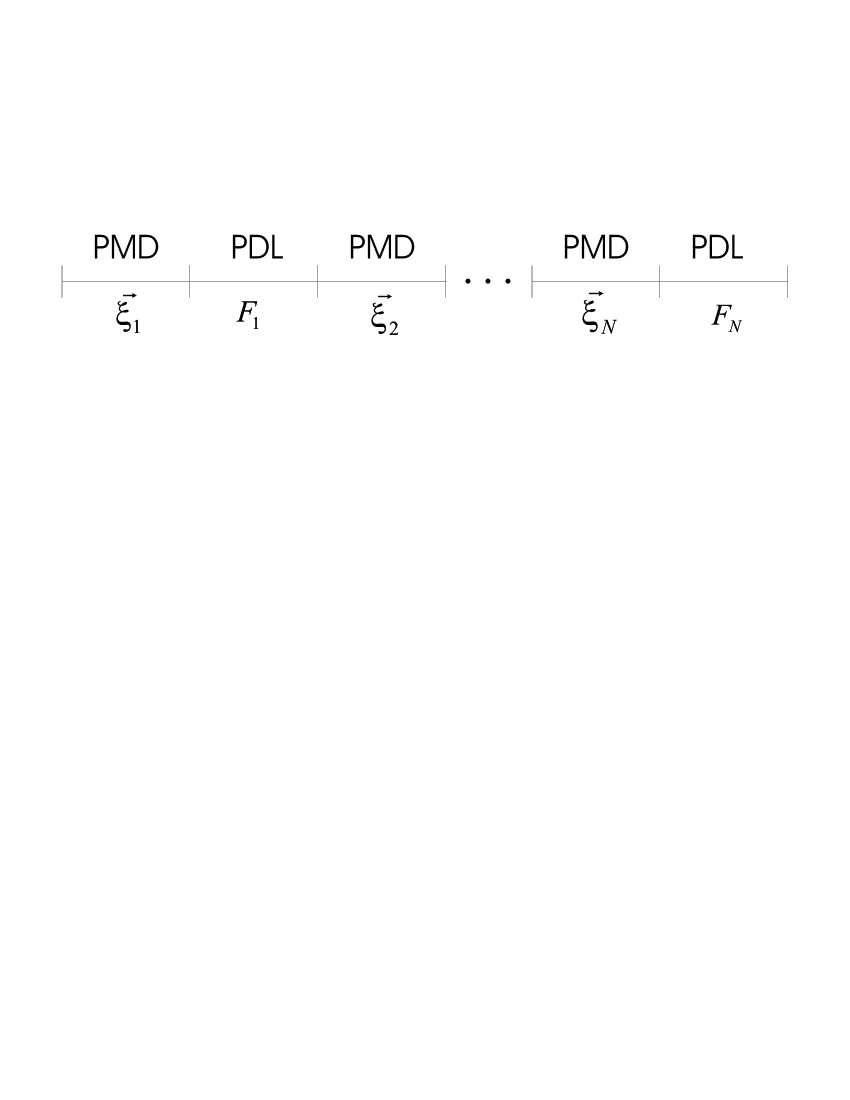
Figure 2: General optical network. A concatenation of PMD and PDL elements.

In this section we show that our work is more than a beautiful analogy and that the quantum formalism can greatly simplify some telecom calculations. We compute the mean time-of-arrival for an arbitrary concatenation of PMD and PDL elements (see Fig.2). Each PMD section is characterized by a birefringence vector $\vec{\xi}_{n}$, its norm being equal to the DGD, $\delta\tau_{n}$, and its direction specifying the measured observable $\frac{1}{\delta\tau_{n}}\,\vec{\xi}_{n}\cdot\vec{\sigma}\equiv\sigma_{n}$. Each PDL element is represented by an operator $F_{n}$. Our input state is again a polarized gaussian pulse $\mbox{$|\Psi_{in}\rangle$}=\mbox{$|g(t)\rangle$}\otimes\mbox{$|\psi\rangle$}$ of central frequency $\omega_{0}$, with coherence time $t_{c}$. Considering energy and polarization degrees of freedom the output state is

$$\mbox{$|\Psi_{out}\rangle$}=F_{N}\,e^{i\omega\frac{\delta\tau_{N}}{2}\sigma_{N}}\cdots F_{1}\,e^{i\omega\frac{\delta\tau_{1}}{2}\sigma_{1}}\,\,\mbox{$|g(t)\rangle$}\otimes\mbox{$|\psi\rangle$}=\prod_{j=N}^{1}F_{j}\,e^{i\omega\frac{\delta\tau_{j}}{2}\sigma_{j}}\,\mbox{$|g(t)\rangle$}\otimes\mbox{$|\psi\rangle$}\,\,.$$ (39)

The product operation has to be carefully defined since operators $F_{j}$ do not commute. We use the notation

$$\prod_{j=1}^{N}F_{j}\equiv F_{1}F_{2}\cdots F_{N}\quad\mbox{and}\quad\prod_{j=N}^{1}F_{j}\equiv F_{N}F_{N-1}\cdots F_{1}\,\,.$$ (40)

As it was shown in section 2, the effect of each PMD section is a spatial separation of the fiber’s eigenmodes and a global rotation around the fiber’s axis. Since both operations commute we can rewrite

$$\mbox{$|\Psi_{out}\rangle$}=\prod_{j=N}^{1}F_{j}\,e^{i\omega\frac{\delta\tau_{j}}{2}\sigma_{j}}\,\mbox{$|g(t)\rangle$}\otimes\mbox{$|\psi\rangle$}=\prod_{j=N}^{1}\tilde{F}_{j}\,e^{i\delta\omega\frac{\delta\tau_{j}}{2}\sigma_{j}}\,\mbox{$|g(t)\rangle$}\otimes\mbox{$|\psi\rangle$}\,\,,$$ (41)

where we have defined $\tilde{F}_{j}\equiv F_{j}\,e^{i\omega_{0}\frac{\delta\tau_{j}}{2}\sigma_{j}}$. Note that $\tilde{F}$ is not self-adjoint. Since we work in the telecom limit of PMD, which we have shown to be equivalent to the regime of weak measurements, all DGD’s $\delta\tau_{n}$ are assumed to be small compared to the coherence time $t_{c}$ of the optical pulse. Therefore the exponential in the above equation can be expanded since $\delta\omega\delta\tau_{j}=\delta\tau_{j}/t_{c}<<1$. We have

$$|\Psi_{out}\rangle \simeq \prod_{j=N}^{1}\tilde{F}_{j}\,(\leavevmode\hbox{\small 1\normalsize\kern-3.30002pt1}+i\delta\omega\frac{\delta\tau_{j}}{2}\sigma_{j})\,\,\mbox{$|g(t)\rangle$}\otimes\mbox{$|\psi\rangle$}$$ (42)

$$= \bigg{[}(\prod_{j=N}^{1}\tilde{F}_{j})+i\delta\omega\sum_{j=1}^{N}\frac{\delta\tau_{j}}{2}F_{N}F_{N-1}\cdots F_{j}\sigma_{j}F_{j-1}\cdots F_{1}\bigg{]}\,\,\mbox{$|g(t)\rangle$}\otimes\mbox{$|\psi\rangle$}\,\,.$$

We now write the state in a well-chosen polarization basis, namely $\big{\{}\prod_{j=N}^{1}\tilde{F}_{j}\mbox{$|\psi\rangle$}\,\,,\,\,\mbox{$|\mbox{orthog}\rangle$}\big{\}}$, where $|\mbox{orthog}\rangle$ is defined by $\mbox{$\langle\mbox{orthog}|$}\prod_{j=N}^{1}\tilde{F}_{j}\mbox{$|\psi\rangle$}=0$ . Note that since $F_{j}$ are non-unitary operations, the state $\prod_{j=N}^{1}\tilde{F}_{j}\mbox{$|\psi\rangle$}$ is not normalized. We write its norm $B\equiv\mbox{$\langle\psi|$}\prod_{j=1}^{N}\tilde{F}_{j}^{{\dagger}}\,\prod_{j=N}^{1}\tilde{F}_{j}\mbox{$|\psi\rangle$}$. In equation (42) we insert the completeness relation

$$\leavevmode\hbox{\small 1\normalsize\kern-3.30002pt1}=\frac{1}{B^{2}}\prod_{j=N}^{1}\tilde{F}_{j}\mbox{$|\psi\rangle$}\mbox{$\langle\psi|$}\prod_{j=1}^{N}\tilde{F}_{j}^{{\dagger}}+\mbox{$|\mbox{orthog}\rangle$}\mbox{$\langle\mbox{orthog}|$}\,\,,$$ (43)

so that

$$|\Psi_{out}\rangle = \frac{1}{B^{2}}\prod_{j=N}^{1}\tilde{F}_{j}\mbox{$|\psi\rangle$}\,\bigg{[}\mbox{$\langle\psi|$}\prod_{j=1}^{N}\tilde{F}_{j}^{{\dagger}}\,\bigg{(}(\prod_{j=N}^{1}\tilde{F}_{j})+i\delta\omega\sum_{j=1}^{N}\frac{\delta\tau_{j}}{2}F_{N}\cdots F_{j}\sigma_{j}F_{j-1}\cdots F_{1}\bigg{)}\bigg{]}\mbox{$|g(t)\rangle$}\otimes\mbox{$|\psi\rangle$}$$ (44)

$$+ \mbox{$|\mbox{orthog}\rangle$}\,\,\bigg{[}\,\mbox{$\langle\mbox{orthog}|$}\,\bigg{(}(\prod_{j=N}^{1}\tilde{F}_{j})+i\delta\omega\sum_{j=1}^{N}\frac{\delta\tau_{j}}{2}F_{N}\cdots F_{j}\sigma_{j}F_{j-1}\cdots F_{1}\bigg{)}\bigg{]}\mbox{$|g(t)\rangle$}\otimes\mbox{$|\psi\rangle$}\,\,.$$

The probability of finding the photon in the state $|\mbox{orthog}\rangle$ is of order $O(\delta\omega\delta\tau_{j})^{2}$, and therefore negligible. So whenever the photon manages to come out it is left in the pure state

$$|\Psi_{out}\rangle = \bigg{[}\,\leavevmode\hbox{\small 1\normalsize\kern-3.30002pt1}+i\delta\omega W\,\bigg{]}\,\bigg{(}\mbox{$|g(t)\rangle$}\otimes(\prod_{j=N}^{1}\tilde{F}_{j}\mbox{$|\psi\rangle$})\bigg{)}$$ (45)

$$\simeq e^{i\delta\omega W}\,\bigg{(}\mbox{$|g(t)\rangle$}\otimes(\prod_{j=N}^{1}\tilde{F}_{j}\mbox{$|\psi\rangle$})\bigg{)}$$

$$= \underbrace{\bigg{(}B\,e^{-\delta\omega Im(W)}\bigg{)}}_{\mbox{attenuation}}\,\,\,\underbrace{\bigg{(}\mbox{$|g(t+Re(W))\rangle$}\otimes(\frac{1}{B}\prod_{j=N}^{1}\tilde{F}_{j}\mbox{$|\psi\rangle$})\bigg{)}}_{\mbox{normalized state }}\,\,,$$

where

$$W=\sum_{j=1}^{N}\frac{\delta\tau_{j}}{2}\,\frac{\mbox{$\langle\psi|$}\prod_{k=1}^{N}\tilde{F}_{k}^{{\dagger}}\,\,\prod_{k=N}^{j+1}\tilde{F}_{k}\,\sigma_{j}\prod_{k=j}^{1}\tilde{F}_{k}\mbox{$|\psi\rangle$}}{\mbox{$\langle\psi|$}\prod_{j=1}^{N}\tilde{F}_{j}^{{\dagger}}\,\prod_{j=N}^{1}\tilde{F}_{j}\,\mbox{$|\psi\rangle$}\,}$$ (46)

So the mean time-of-arrival is

$$\langle t\rangle=\sum_{j=1}^{N}\frac{\delta\tau_{j}}{2}\,Re\bigg{(}\frac{\mbox{$\langle\psi|$}\prod_{k=1}^{N}\tilde{F}_{k}^{{\dagger}}\,\,\prod_{k=N}^{j+1}\tilde{F}_{k}\,\sigma_{j}\prod_{k=j}^{1}\tilde{F}_{k}\mbox{$|\psi\rangle$}}{\mbox{$\langle\psi|$}\prod_{j=1}^{N}\tilde{F}_{j}^{{\dagger}}\,\prod_{j=N}^{1}\tilde{F}_{j}\,\mbox{$|\psi\rangle$}\,}\bigg{)}\,\,.$$ (47)

Note that the state (45) is not normalized because of the losses in the system, and that the attenuation depends on the central frequency of the pulse $\omega_{0}$. Expression (47) may seem quite cumbersome but can be rewritten in a far more intuitive way. We define the following notation

$$w(\vec{\xi_{j}},\mbox{$|\psi\rangle$},\rho)\equiv\frac{\delta\tau_{j}}{2}Re\bigg{(}\frac{\mbox{$\langle\psi|$}\rho\,\sigma_{j}\mbox{$|\psi\rangle$}}{\mbox{$\langle\psi|$}\rho\mbox{$|\psi\rangle$}}\bigg{)}\,\,.$$ (48)

So $w(\vec{\xi},\mbox{$|\psi\rangle$},\rho)$ is the mean time shift of a PMD section with birefringence vector $\vec{\xi}$ when the input state is $|\psi\rangle$ and the post-selection is done on the mixed state $\rho$. With this, equation (47) reads

$$\langle t\rangle = w\big{(}\vec{\xi}_{1}\,,\,\mbox{$|\psi\rangle$}\,,\,\tilde{F}_{1}^{{\dagger}}\cdots\tilde{F}_{N}^{{\dagger}}\tilde{F}_{N}\cdots\tilde{F}_{1}\big{)}\,+\,w\big{(}\vec{\xi}_{2}\,,\,\tilde{F}_{1}\mbox{$|\psi\rangle$}\,,\,\tilde{F}_{2}^{{\dagger}}\cdots\tilde{F}_{N}^{{\dagger}}\tilde{F}_{N}\cdots\tilde{F}_{2}\big{)}$$ (49)

$$+\cdots+\,w\big{(}\vec{\xi}_{N}\,,\,\tilde{F}_{N-1}\cdots\tilde{F}_{1}\mbox{$|\psi\rangle$}\,,\,\tilde{F}_{N}^{{\dagger}}\tilde{F}_{N}\big{)}$$

So the mean time-of-arrival is simply the sum of the contributions of each PMD section computed when forgetting about all others PMD’s. This is quite natural since all PMD’s are assumed to be weak measurements, which means they modify only slightly the shape of the pulse ($\delta\tau_{j}<<t_{c}$ $\forall j$).

So we obtain an analytical formula for the mean time-of-arrival for an arbitrary concatenation of PMD and PDL elements. It should be stressed that the structure of this formula is very simple. In this sense we feel our analogy simplifies telecom calculation since the equivalent computation in the usual PMD-PDL language is less straightforward.

Another important result of [2] was that any concatenation of PMD and PDL elements is equivalent to a simple setup where an effective PMD is followed by an effective frequency-dependent PDL. This is a consequence of the polar decomposition theorem for complex matrices, which states that any complex matrix $T$ can be decomposed into a unitary matrix $U$ and a positive Hermitian one $A$, so that $T=AU$. Unfortunately we were unable to recover this result in the quantum formalism.

5.2 Optimal concatenation problem

To illustrate the transparency of the structure of equation (49), we discuss the following problem. How should one assemble a given number of PMD and PDL sections in order to maximize (or minimize) the mean time-of-arrival $\langle t\rangle$? In other words which setup optimizes the interaction between PMD and PDL. For definiteness, we consider a five elements PMD-PDL-PMD-PDL-PMD network. We omit all rotations due to PMD sections, because they clearly play no role in our problem. Note that anyway, one could change the lengths of each PMD element so that the rotation due to PMD is a multiple of $2\pi$. Using equation (49) we have

$$\langle t\rangle=\frac{\delta\tau_{1}}{2}\,\frac{\mbox{$\langle\psi|$}F_{1}F_{2}^{2}F_{1}\,\sigma_{1}\mbox{$|\psi\rangle$}}{\mbox{$\langle\psi|$}F_{1}F_{2}^{2}F_{1}\,\mbox{$|\psi\rangle$}}+\frac{\delta\tau_{2}}{2}\,\frac{\mbox{$\langle\psi|$}F_{1}F_{2}^{2}\,\sigma_{2}F_{1}\,\mbox{$|\psi\rangle$}}{\mbox{$\langle\psi|$}F_{1}F_{2}^{2}F_{1}\,\mbox{$|\psi\rangle$}}+\frac{\delta\tau_{3}}{2}\,\frac{\mbox{$\langle\psi|$}F_{1}F_{2}\,\sigma_{2}F_{2}F_{1}\,\mbox{$|\psi\rangle$}}{\mbox{$\langle\psi|$}F_{1}F_{2}^{2}F_{1}\,\mbox{$|\psi\rangle$}}$$ (50)

Numerical simulations show that in order to maximize $\langle t\rangle$, one has to align respectively all PMD’s and all PDL’s and choose the PDL axis orthogonal to the PMD axis. Now one question remains: should the PDL be distributed all along the network or simply grouped at the end of the setup. It turns out that the second choice is better (see Fig.3) and our formula clearly shows why. From the three terms of equation (50) the first one is the largest, since all filters contribute to the post-selection. But this first term is precisely the contribution of the setup where all the PDL is at the end. Thus $\langle t\rangle$ is maximized whenever the weight of the first term (say $\delta\tau/2$) is the largest. This is of course the case when all PMD’s sections are put together. Since they are all parallel, we have $\delta\tau/2=\sum_{j=1}^{N}\delta\tau_{j}/2$.

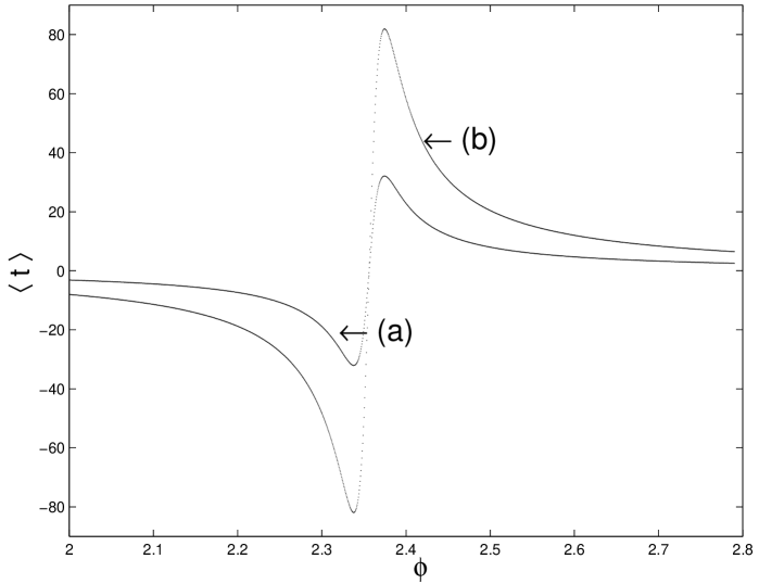
Figure 3: Mean time-of-arrival $\langle t\rangle$ versus polarization (we consider linear polarizations $\mbox{$|\psi\rangle$}=\cos(\phi/2)\mbox{$|H\rangle$}+\sin(\phi/2)\mbox{$|V\rangle$}$). In this example we used: $\delta\tau_{j}=1$, for $j=1,2,3$ and $\mu_{j}=1$ for $j=1,2$. (a) Five elements PMD-PDL-PMD-PDL-PMD network. The PDL is distributed along the line. (b) PMD(3)-PDL(2) setup. All PMD (PDL) sections are grouped at the beginning (at the end) of the setup. The time shift can be made nearly three times larger with this second setup.

6 Conclusion

In conclusion, we have demonstrated that the formalism of weak measurements with post-selection describes important polarization effects in the physics of telecom optics. It is quite nice and surprising to see that telecom engineers and quantum theorists, two apparently completely unconnected categories of physicist, speak of the same things, each one in his own language. We also showed that the quantum formalism simplifies telecom calculations and gives a better understanding of the physics of networks. It must also be mentioned that with this work we close a loop of analogies. On the one hand, Gisin and Go showed in [7] the strong analogy between PMD-PDL effects in networks, and the mixing and decay that are intrinsic to kaons. Remember that the kaon system is one of the most celebrated examples of a system evolving according to an effective non hermitian Hamiltonian. On the other hand, it was shown in [8] that a system coupled to another suitably pre- and post-selected system can also evolve according to an effective non hermitian Hamiltonian. So our work closes the loop by showing the link between PMD-PDL effects and weak measurements with post-selection.

References

• [1] Y. Aharonov and L. Vaidman, Quant. phys. (2001); published in: J.G. Muga, R. Sala Mayoto and I.L. Egusquiza (eds), Time in quantum Mechanics, Lecture Notes in Physics, (Springer Verlag, 2002)
• [2] B. Huttner, C. Geiser and N. Gisin, IEEE J. Sel. Top. Quantum Electron. 6, 317 (2000).
• [3] S. Huard, Polarisation de la lumi re (Masson, Paris, 1994).
• [4] Y. Aharonov, P.G. Bergmann and J.L. Lebowitz, Phys. Rev. B 134, 1410 (1964)
• [5] A. Peres, Quantum Theory: Concepts and Methods (Kluwer, Dordrecht, 1998), section 9-5
• [6] B. Huttner et al., Phys. Rev. A 54, 3783 (1996)
• [7] N. Gisin, A. Go, Am. J. Phys. 69, 264 (2001)
• [8] Y. Aharonov et al., Phys. Rev. Lett. 77, 983 (1996)