Solvable model of a strongly-driven micromaser

Abstract

We study the dynamics of a micromaser where the pumping atoms are strongly driven by a resonant classical field during their transit through the cavity mode. We derive a master equation for this strongly-driven micromaser, involving the contributions of the unitary atom-field interactions and the dissipative effects of a thermal bath. We find analytical solutions for the temporal evolution and the steady-state of this system by means of phase-space techniques, providing an unusual solvable model of an open quantum system, including pumping and decoherence. We derive closed expressions for all relevant expectation values, describing the statistics of the cavity field and the detected atomic levels. The transient regime shows the build-up of mixtures of mesoscopic fields evolving towards a superpoissonian steady-state field that, nevertheless, yields atomic correlations that exhibit stronger nonclassical features than the conventional micromaser.

I Introduction

The micromaser m.m. is a fundamental system in cavity quantum electrodynamics (CQED) qed where a single cavity mode is pumped by a poissonian beam of excited two-level atoms, in such a way that at most one atom is inside the cavity. While each atom traverses the cavity, the entangled atom-cavity system undergoes the Jaynes-Cummings (JC) interaction JC and, when this is not the case, the field decays due to its coupling to the environment. It has been demonstrated that the micromaser exhibits interesting nonclassical features in the field statistics and in the atomic correlations, like subpoissonian photon statistics subp , trapping states TS and number states Fock of the cavity field, and antibunched atomic correlations Englert1 .

Recently, it was shown that the effective coupling between an atom and a single cavity mode can be drastically modified in the presence of a strong external driving field SAW . For example, under resonant conditions among the atomic transition, the cavity mode and the external field, it is possible to engineer a resonant JC and anti-JC interaction simultaneously. In this case, the usual atom-field Rabi oscillations do not play any further role, leaving their place to conditional field displacements depending on the atomic internal states: “Schrödinger cat states.” Generation of entanglement and its measurement is a very active field in CQED with diverse implications in fundamental and applied quantum physics Englert1 ; Haroche . From that point of view, a more realistic study of this new scheme and its different variants, where dissipative effects are fully taken into account, is desirable.

In this paper we develop the theory of a strongly-driven micromaser (SDM) and study the new features of the field statistics and the atomic correlations. We formulate a master equation for the cavity field density operator where the gain originates in the coherent interaction of the field with two-level atoms which are strongly driven by an external driving while they are inside the cavity SAW . The losses in the master equation stem from the interaction of the cavity field with a thermal bath. The additional strong driving acting on the atoms changes drastically the SDM dynamics as compared with the conventional micromaser.

We show that the SDM master equation can be solved analytically by means of phase-space methods, providing an unusual solvable model of an open quantum system under realistic conditions. In this way we are able to trace the temporal evolution of the SDM field from an arbitrary initial state to the final steady-state, which happens to be superpoissonian. We derive closed expressions for the main quantities which characterize the statistics of the cavity photons and the detected atoms. We find that, despite the classicality of the SDM field steady-state, the atomic correlations exhibit stronger nonclassical features when compared with the conventional micromaser. The description of system dynamics is illustrated also by numerical results which support and complement the analytical ones. It is worth noting that the present SDM system differs markedly from the recently investigated coherently-driven micromaser CL , where an external field continuously drives the cavity mode and no strong driving regime is required.

In Sec. II, we present the atom-field Hamiltonian of the SDM and illustrate its main dynamical features. In particular, we show how the cavity field changes as a consequence of the passage of one, two, or more atoms. We pay careful attention to the crucial difference between the situations in which the atoms remain unobserved and in which their final state is detected. Then, in Sec. III, we formulate the SDM master equation and derive its time-dependent analytical solution. As an application, we use it to calculate the expectation values of various important observables of the photon field, and of the atom counting statistics. Numerical results are discussed in Sec. IV, and conclusions are drawn in Sec. V.

II Hamiltonian and coherent dynamics

The fully resonant interaction between one mode of a high-Q cavity and a two-level atom strongly driven by a classical external field can be described by the following Hamiltonian SAW

$$H=\frac{\hbar g}{2}(\sigma^{\dagger}+\sigma)(a^{\dagger}+a),$$ (1)

where $g$ is the atom-cavity mode coupling constant, $a$ ($a^{\dagger}$) the field annihilation (creation) operator, and $\sigma=|g\rangle\langle e|$ ($\sigma^{\dagger}=|e\rangle\langle g|$) the atomic lowering (raising) operator. The Hamiltonian of Eq. (1), written in the interaction picture, was derived in SAW in the strong driving regime $\Omega\gg g$, where $\Omega$ is the Rabi frequency associated with the external field.

A first feature of Hamiltonian in Eq. (1) is the presence of resonant terms of both the Jaynes-Cummings type, $\sigma^{\dagger}a+\sigma a^{\dagger}$, and of the anti-JC type, $\sigma^{\dagger}a^{\dagger}+\sigma a$. Actually, the latter terms are usually negligible in CQED, whereas they can be of importance in other systems, like ion traps ion . A second feature, that is discussed below, is the direct generation of the so-called Schrödinger cat states of the cavity field.

The Hamiltonian of Eq. (1) generates a time evolution that is described by the unitary operator

$$U(\xi)=D(\xi)|+\rangle\langle+|+D(-\xi)|-\rangle\langle-|\,,$$ (2)

where the parameter $\xi=-ig\tau/2$ is proportional to the interaction time $\tau$; $D(\alpha)=\exp{(\alpha a^{\dagger}-\alpha^{*}a)}$ is the unitary displacement operator; and $|\pm\rangle=(1/\sqrt{2})(|g\rangle\pm|e\rangle)$ are the eigenstates of the atomic operator $\sigma_{x}\equiv\sigma^{\dagger}+\sigma$ with eigenvalues $\pm 1$, respectively. Starting from an initial state with the cavity field in a state $\rho_{F,0}$ and one atom injected in the excited state,

$$\rho_{0}=\rho_{F,0}\otimes|e\rangle\langle e|\,,$$ (3)

the density operator evolves to the state

$$\rho_{1}=U(\xi)\rho_{0}U(-\xi)\,.$$ (4)

We consider two cases, one in which the atom is not observed when it leaves the cavity and the other in which it is detected in the upper or lower level.

II.1 Atoms are not observed

If we are interested in the cavity field after the atomic transit without measuring the state of the outgoing atom, the cavity field density operator is

$$\rho_{F,1}=\mathrm{Tr}_{A}\rho_{1}=\frac{1}{2}\left[D(\xi)\rho_{F,0}D(-\xi)+D(-\xi)\rho_{F,0}D(\xi)\right]\,,$$ (5)

where $\mathrm{Tr}_{A}$ is the partial trace over the atomic degrees of freedom, and we used Eqs. (2)-(4). If the cavity is initially in the vacuum state, $\rho_{F,0}=|0\rangle\langle 0|$, its state turns into

$$\rho_{F,1}=\frac{1}{2}\left(|\xi\rangle\langle\xi|+|-\xi\rangle\langle-\xi|\right)\,,$$ (6)

which is a statistical mixture of two coherent states with the same amplitude and opposite phases.

It is of interest for what follows to describe the time evolution of the cavity field in phase space. While for the vacuum state the Wigner function is the Gaussian $W_{0}(\alpha)=2\exp{(-2|\alpha|^{2})}$, for the state of Eq. (6) we have

$$W_{1}(\alpha)=2\exp{\left[-2(|\alpha|^{2}+|\xi|^{2})\right]}\cosh(4|\xi|\mathrm{Im}\,\alpha)\,.$$ (7)

This last expression shows that the interaction with a driven atom can affect the rotational symmetry of the initial vacuum state. The section of $W_{1}(\alpha)$ along the real axis remains a Gaussian with the initial minimum uncertainty, while the section along the imaginary axis is broadened, showing a two-peaked structure that results from the superposition of two Gaussians centered at $\alpha=\pm\xi$. The two peaks are well resolved if $|\xi|\gg 1/2$, which requires that the system is operated in the strong-coupling regime $(g\tau\gg 1)$.

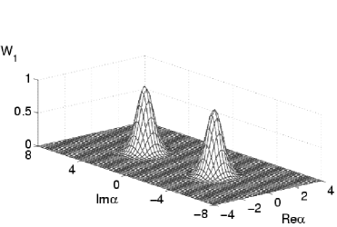
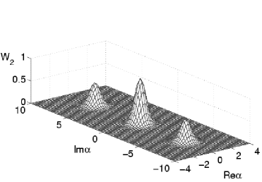
Figure 1: Wigner distributions $W_{1}(\alpha)$ and $W_{2}(\alpha)$ of the cavity field, see Eq. (9), in the case of one and two crossing atoms, respectively, provided that no attempt is made to determine the final internal state of the atoms. Here, as well as in all the following figures, $|\xi|=\pi$, the cavity field is initially in the vacuum state, and the atoms in the excited state.

If the cavity mode, initially in the vacuum state, interacts with $1,2,\ldots,m$ strongly driven atoms, all assumed to pass through the cavity (one by one) with the same interaction time $\tau$ and to leave it unobserved, the final field state is given by the density operator

$$\rho_{F,m}=\frac{1}{2^{m}}\sum_{n=0}^{m}\left(\begin{array}[]{c}m\\ n\end{array}\right)|(m-2n)\xi\rangle\langle(m-2n)\xi|\,,$$ (8)

which describes a mixture of $m+1$ coherent states. This state is represented in phase space by the Wigner function

$$W_{m}(\alpha)=\frac{1}{{2^{m-1}}}\sum_{n=0}^{m}\left(\begin{array}[]{c}m\\ n\end{array}\right)\exp{\left[-2|\alpha-(m-2n)\xi|^{2}\right]}\,.$$ (9)

Hence, in the strong coupling regime and with negligible dissipation effects, multi-peaked cavity field distributions can be generated in phase-space, where the number of peaks increases with the number of driven atoms injected in the cavity. The subsequent generation of such cavity field states is illustrated in Fig. 1, where we show the Wigner functions $W_{1}(\alpha),W_{2}(\alpha)$ calculated from Eq. (9). After the transit of m atoms the function $W_{m}(\alpha)$ exhibits $m+1$ peaks, all centered on the imaginary axis and with a center-to-center distance of $2|\xi|=g\tau$. If $m$ is even, the peaks are centered at $\mathrm{Re}\alpha=0$ and $\mathrm{Im}\alpha=0,\pm 2|\xi|,\ldots,$ where the central peak in the origin is the highest one. If $m$ is odd, the centers are at $\mathrm{Re}\alpha=0$ and $\mathrm{Im}\alpha=\pm|\xi|,\pm 3|\xi|,\ldots$, the highest peaks being at $\alpha=\pm\xi$.

II.2 Atoms are detected

Now we consider the cavity field in the case in which the strongly driven atoms are detected when they leave the cavity, e.g. their state is determined by selective field ionization, where for simplicity we assume perfect detector efficiency. We are again interested in the cavity field properties after interaction. Proceeding again from the initial condition of Eq. (3), and using Eqs. (2)-(4), the cavity field density operators after detecting the atom in the excited state ${\rho}^{(e)}_{F,1}$ or in the ground state ${\rho}^{(g)}_{F,1}$ are

$${\rho}^{(e)}_{F,1} = \frac{\left[D(\xi)+D(-\xi)\right]\rho_{F,0}\left[D(\xi)+D(-\xi)\right]}{2\left[\mathrm{Re}\chi(2\xi)+1\right]}\,,$$

$${\rho}^{(g)}_{F,1} = \frac{\left[D(\xi)-D(-\xi)\right]\rho_{F,0}\left[D(\xi)-D(-\xi)\right]}{2\left[\mathrm{Re}\chi(2\xi)-1\right]}\,,$$ (10)

where $\chi(\beta)=\mathrm{Tr}_{F}\left\{\rho_{F,0}D(\beta)\right\}$ is the characteristic function for symmetrical ordering of the field operators CG and $\mathrm{Tr}_{F}$ is the partial trace over the field variables. If the cavity is initially in the vacuum state, then

$${\rho}^{(e)}_{F,1}=\frac{|\xi\rangle\langle\xi|+|-\xi\rangle\langle-\xi|+|\xi\rangle\langle-\xi|+|-\xi\rangle\langle\xi|}{2\left[1+\exp(-2|\xi|^{2})\right]}\,,$$

$${\rho}^{(g)}_{F,1}=\frac{|\xi\rangle\langle\xi|+|-\xi\rangle\langle-\xi|-|\xi\rangle\langle-\xi|-|-\xi\rangle\langle\xi|}{2\left[1-\exp(-2|\xi|^{2})\right]}\,,$$

which are pure states of the cavity field instead of the statistical mixtures of Eq. (6). Actually, the cavity field state vectors are ${|{\psi}_{F,1}\rangle}^{(e),(g)}\propto(|\xi\rangle\pm(|-\xi\rangle)$, that is the superposition of two coherent states of the kind generated and monitored in the dispersive regime of cavity QED in cats . More elaborated superposition states were investigated in Ref. SAW , where also many-atom states were considered. The mean photon number of the field states of Eq. (II.2) are

$${\langle N_{1}\rangle}^{(e),(g)}={|\xi|^{2}}\frac{1\mp\exp(-2|\xi|^{2})}{1\pm\exp(-2|\xi|^{2})}\,,$$ (12)

whereas $\langle N_{1}\rangle=|\xi|^{2}$ in the case of an unmeasured atom of Sec. II.1.

The Wigner functions representing the states of Eq. (II.2) are

$$W^{(e),(g)}_{1}(\alpha) = 2e^{-2|\alpha|^{2}}\bigl{[}e^{-2|\xi|^{2}}\cosh(4|\xi|\mathrm{Im}\,\alpha)$$ (13)

$$\pm\cos(4|\xi|\mathrm{Re}\,\alpha)\bigr{]}/\bigl{(}1\pm e^{-2|\xi|^{2}}\bigr{)}\,.$$

Beyond the two-peaked structure, present in Eq. (7) for an unmeasured atom (see also Fig. 1), the presence of the sinusoidal interference term implies that the Wigner functions in Eq. (13) can exhibit strong oscillations with period $\pi/2|\xi|$. They can even take negative values (see Fig. 2), which is a signature of the quantum nature of the cavity field states of Eq. (II.2). In particular, in the origin of phase space, $W^{(e),(g)}_{1}(0)=\pm 2$.

(a)

(b)

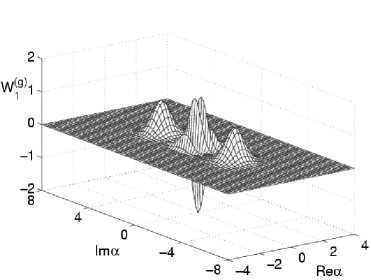
Figure 2: Wigner distribution of the cavity field for the case of one crossing atom detected (a) in the excited state, $W_{1}^{(e)}(\alpha)$; (b) in the ground state, $W_{1}^{(g)}(\alpha)$; see Eq. (13).

If a second atom crosses the cavity and is also detected in the upper or lower state soon after, the cavity field is projected onto one of the following states,

$${\rho}^{(ee)}_{F,2} = \bigl{[}|2\xi\rangle\langle 2\xi|+4|0\rangle\langle 0|+|-2\xi\rangle\langle-2\xi|+|2\xi\rangle\langle-2\xi|$$

$$+|-2\xi\rangle\langle 2\xi|+2(|2\xi\rangle\langle 0|+|0\rangle\langle 2\xi|+|0\rangle\langle-2\xi|$$

$$+|-2\xi\rangle\langle 0|)\bigr{]}\Big{/}\bigl{[}2(3+4e^{-2|\xi|^{2}}+e^{-8|\xi|^{2}})\bigr{]}\,,$$

$${\rho}^{(eg)}_{F,2} = {\rho}^{(ge)}_{F,2}=\bigl{[}|2\xi\rangle\langle 2\xi|+|-2\xi\rangle\langle-2\xi|$$

$$-|2\xi\rangle\langle-2\xi|-|-2\xi\rangle\langle 2\xi|\bigr{]}\Big{/}\bigl{[}2(1-e^{-8|\xi|^{2}})\bigr{]}\,,$$

$${\rho}^{(gg)}_{F,2} = \bigl{[}|2\xi\rangle\langle 2\xi|+4|0\rangle\langle 0|+|-2\xi\rangle\langle-2\xi|+|2\xi\rangle\langle-2\xi|$$

$$+|-2\xi\rangle\langle 2\xi|-2(|2\xi\rangle\langle 0|+|0\rangle\langle 2\xi|+|0\rangle\langle-2\xi|$$

$$+|-2\xi\rangle\langle 0|)\bigr{]}\Big{/}\bigl{[}2(3-4e^{-2|\xi|^{2}}+e^{-8|\xi|^{2}})\bigr{]}\,,$$

where, for instance, (eg) means that the first atom is detected in the upper state and the second one in the lower state. The expressions of Eq. (II.2) should be compared with the statistical mixture of Eq. (8) in the case of two unobserved atoms ($m=2$). The density operators in Eq. (II.2) describe mesoscopic Schrödinger-cat-like states of the cavity field, the corresponding state vectors being

$${|{\psi}_{F,2}\rangle}^{(ee),(gg)} \propto (|2\xi\rangle\pm 2|0\rangle+|-2\xi\rangle)\,,$$

$${|{\psi}_{F,2}\rangle}^{(eg)}={|{\psi}_{F,2}\rangle}^{(ge)} \propto (|2\xi\rangle-|-2\xi\rangle)\,.$$ (15)

The Wigner functions which represent the above states in phase space, whose behavior is depicted in Fig. 3, can be written as

$$W^{(ee)}_{2}(\alpha) = 2e^{-2|\alpha|^{2}}\bigl{[}2+e^{-8|\xi|^{2}}\cosh(8|\xi|\mathrm{Im}\,\alpha)$$

$$+4e^{-2|\xi|^{2}}\cosh(4|\xi|\mathrm{Im}\,\alpha)\cos(4|\xi|\mathrm{Re}\,\alpha)$$

$$+\cos(8|\xi|\mathrm{Re}\,\alpha)\bigr{]}\Big{/}\bigr{(}3+4e^{-2|\xi|^{2}}+e^{-8|\xi|^{2}}\bigr{)}\,,$$

$$W^{(eg)}_{2}(\alpha) = W^{(ge)}_{2}(\alpha)=2e^{-2|\alpha|^{2}}\bigl{[}-\cos(8|\xi|\mathrm{Re}\,\alpha)$$

$$+e^{-8|\xi|^{2}}\cosh(8|\xi|\mathrm{Im}\alpha)\bigr{]}\Big{/}\bigl{(}1-e^{-8|\xi|^{2}}\bigr{)}\,,$$

$$W^{(gg)}_{2}(\alpha) = 2e^{-2|\alpha|^{2}}\bigl{[}2+e^{-8|\xi|^{2}}\cosh(8|\xi|\mathrm{Im}\,\alpha)$$

$$-4e^{-2|\xi|^{2}}\cosh(4|\xi|\mathrm{Im}\alpha)\cos(4|\xi|\mathrm{Re}\,\alpha)$$

$$+\cos(8|\xi|\mathrm{Re}\,\alpha)\bigr{]}\Big{/}\bigl{(}3-4e^{-2|\xi|^{2}}+e^{-8|\xi|^{2}}\bigr{)}\,.$$

(a)

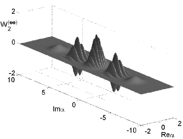
(b)

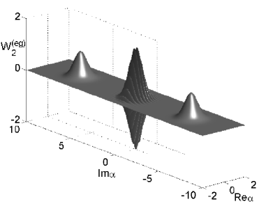
(c)

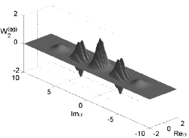
Figure 3: Wigner distribution of the cavity field for the case of two crossing atoms detected (a) both in the excited state, $W_{2}^{(ee)}(\alpha)$; (b) one in the excited state and the other in the ground state, $W_{2}^{(eg)}(\alpha)$; (c) both in the ground state, $W_{2}^{(gg)}(\alpha)$; see Eq. (II.2).

We consider now the atomic statistics at the exit of the cavity independent of the cavity field state. If an atom is injected in the cavity, so that the initial state is $\rho_{F}\otimes|e\rangle\langle e|$, the atomic state after the interaction will be

$$\rho_{A} = \mathrm{Tr}_{F}\bigl{\{}U(\xi)\rho_{F}\otimes|e\rangle\langle e|U(-\xi)\bigr{\}}$$ (17)

$$= \frac{1}{2}\Bigl{[}1_{A}+\mathrm{Re}\,\chi(2\xi)\bigl{(}|e\rangle\langle e|-|g\rangle\langle g|\bigr{)}$$

$$+i\,\mathrm{Im}\,\chi(2\xi)\bigl{(}|g\rangle\langle e|-|e\rangle\langle g|\bigr{)}\Bigr{]}\,.$$

Here, $\mathrm{Tr}_{F}$ is the partial trace over the cavity mode degrees of freedom. In the derivation of Eq. (17) we used also Eqs. (2) and (3) as well as the property $\chi(\beta)=\chi(-\beta)^{*}$. Finally, we can calculate the probability $p_{e,g}$ for atomic detection in the upper or lower state as

$$p_{e,g}=\langle e,g|\rho_{A}|e,g\rangle=\frac{1}{2}\bigl{[}1\pm\,\mathrm{Re}\,\chi(2\xi)\bigr{]}\,.$$ (18)

III Master equation and analytical results

III.1 SDM master equation and analytical solutions

We consider now the case of a poissonian beam of two-level Rydberg atoms, with pumping rate $r$, interacting with a single mode of a microwave high-Q cavity. While the atoms are inside the cavity, during an interaction time $\tau$, they are strongly driven by an additional classical field, the whole system being in resonance. We study a regime where at most one atom is present inside the cavity, that is, $\tau\ll r^{-1}$, and where the decay of atomic Rydberg levels is negligible. Between two successive atoms, the cavity field decays due to its interaction with a thermal bath. Hence, even though the present strongly-driven micromaser (SDM) looks quite similar to the conventional micromaser, there is a crucial difference in the pumping dynamics. As we discussed in the previous section, the JC interaction and its Rabi oscillations do not rule any more the unitary atom-field interaction. Their role is taken over by field displacements conditioned on the atomic internal states.

The dynamics of the SDM field is ruled by the interplay between the amplification process, due to the interaction with the driven atoms, and the dissipation process, occurring when no atom crosses the cavity. In a coarse-grained description the gain rate of the cavity mode follows from Eq.(5),

$$\frac{\partial\rho_{F}}{\partial t}\Bigg{|}_{\mathrm{gain}}=\frac{r}{2}\bigl{[}D(\xi)\rho_{F}D(-\xi)+D(-\xi)\rho_{F}D(\xi)-2\rho_{F}\bigr{]}\,.$$ (19)

The loss rate, due to the interaction of the cavity field with a thermal bath SZ , is given by

$$\frac{\partial\rho_{F}}{\partial t}\Bigg{|}_{\mathrm{loss}} = -\frac{\gamma(\bar{n}+1)}{2}\bigl{[}a^{\dagger}a\rho_{F}-2a\rho_{F}a^{\dagger}+\rho_{F}a^{\dagger}a\bigr{]}$$

$$-\frac{\gamma\bar{n}}{2}\bigl{[}aa^{\dagger}\rho_{F}-2a^{\dagger}\rho_{F}a+\rho_{F}aa^{\dagger}\bigr{]}\equiv\mathcal{L}\rho_{F}\,,$$

where $\gamma$ is the cavity photon decay rate and $\bar{n}$ the mean thermal photon number. By combining Eqs. (19) and (III.1) we obtain the SDM master equation

$$\frac{\partial\rho_{F}}{\partial t}=\frac{r}{2}[D(\xi)\rho_{F}D(-\xi)+D(-\xi)\rho_{F}D(\xi)-2\rho_{F}]+\mathcal{L}\rho_{F}\,.$$ (21)

At variance with the conventional micromaser, whose master equation has only an analytical solution in steady-state Meystre , the SDM master equation (21) can be fully solved for any time. The key step is a transformation of the equation of motion (21) for the density operator into the corresponding partial differential equation for its symmetrically ordered characteristic function $\chi(\beta)$, already introduced in the previous section. We recall that $\chi(\beta)$ is related to the field density operator by CG

$$\rho_{F}=\pi^{-1}\int\chi(\beta)D^{-1}(\beta)\,d^{2}\beta\,$$ (22)

and that the Wigner function, $W(\alpha)$, is the 2D Fourier transform of the characteristic function $\chi(\beta)$ CG .

Using known operator techniques SZ , we thus map Eq. (21) into the following partial differential equation for $\chi(\beta,\beta^{*},t)$,

$$\frac{\partial}{\partial t}\chi(\beta,\beta^{*},t) = \Bigl{[}\frac{r}{2}\bigl{(}e^{\xi^{*}\beta-\xi\beta^{*}}+e^{-\xi^{*}\beta+\xi\beta^{*}}-2\bigr{)}$$

$$-\frac{\gamma}{2}(2\bar{n}+1)|\beta|^{2}\Bigr{]}\chi(\beta,\beta^{*},t)$$

$$\mbox{}-\frac{\gamma}{2}\Bigl{(}\beta\frac{\partial}{\partial\beta}+\beta^{*}\frac{\partial}{\partial\beta^{*}}\Bigr{)}\chi(\beta,\beta^{*},t)\,.$$

We transform Eq. (III.1) to cartesian coordinates by setting $\xi^{*}\beta\equiv|\xi|(x+iy)$, which gives

$$\biggl{(}\frac{\partial}{\partial t}+\frac{\gamma}{2}\Bigl{[}x\frac{\partial}{\partial x}+y\frac{\partial}{\partial y}+xG^{\prime}(x)+yF^{\prime}(y)\Bigr{]}\biggr{)}\chi(x,y,t)=0\,,$$ (24)

where

$$G(x) = \frac{2\bar{n}_{b}+1}{2}x^{2}\,,$$

$$F(y) = \int\limits^{y}_{0}\frac{4N_{ex}\sin^{2}(|\xi|z)+(2\bar{n}_{b}+1)z^{2}}{z}dz\,,$$ (25)

and $N_{ex}=r/{\gamma}$. The solution of Eq. (24) reads

$$\chi(x,y,t)=\frac{\chi^{\mathrm{(ss)}}(x,y)\chi_{0}(xe^{-\frac{\gamma t}{2}},ye^{-\frac{\gamma t}{2}})}{\chi^{\mathrm{(ss)}}(xe^{-\frac{\gamma t}{2}},ye^{-\frac{\gamma t}{2}})}.$$ (26)

Here,

$$\chi^{\mathrm{(ss)}}(x,y)=e^{-G(x)-F(y)}$$ (27)

is the steady-state solution of Eq. (24) that is reached for $t\rightarrow\infty$, and $\chi_{0}=\mathrm{Tr}_{F}[\rho_{F}(0)D]$ is the characteristic function corresponding to the initial field state $\rho_{F}(0)$. By substituting the expressions of Eq. (III.1) into Eq. (27), we arrive at the steady-state characteristic function

$$\chi^{\mathrm{(ss)}}(x,y) = \exp\Bigl{(}-(\bar{n}+{\textstyle\frac{1}{2}})(x^{2}+y^{2})$$

$$+4N_{ex}\bigl{[}-\gamma_{e}-\ln(2|\xi|y)+\mathrm{Ci}(2|\xi|y)\bigr{]}\Bigr{)}\,,$$

where $\gamma_{e}$ is Euler’s constant and $\mathrm{Ci}(2|\xi|y)$ is the Cosine Integral defined as

$$\mathrm{Ci}(2|\xi|y)=\gamma_{e}+\ln(2|\xi|y)+\int\limits^{2|\xi|y}_{0}\frac{\cos(z)-1}{z}dz\,.$$ (29)

Note that starting from a real initial function, the time-dependent solution in Eq. (26) will always produce a real characteristic function. This follows from the invariance of the time evolution equation in Eq. (III.1) under the transformation $\beta\rightarrow-\beta$, and from the property $\chi(\beta)=\chi(-\beta)^{*}$. Accordingly, the solution of Eq. (26) depends only on the modulus of the (imaginary) parameter $\xi$, which is in agreement with the invariance of the master equation (21) under the transformation $\xi\rightarrow-\xi$.

III.2 SDM field statistics

It is clear that from the general solution of the characteristic function, Eq. (26), we can calculate the field density operator $\rho_{F}(t)$, following Eq. (22), and have access to the field statistics. However, this information can be directly extracted from the characteristic function itself, since the expectation value of any symmetrically ordered product of the operators $a$ and $a^{\dagger}$ is given by CG

$$\langle(a^{\dagger})^{m}a^{n}\rangle_{\mathrm{sym}}=\frac{\partial^{m+n}\chi(\beta,\beta^{*})}{\partial\beta^{m}\partial(-\beta^{*})^{n}}\bigg{|}_{\beta=\beta^{*}=0}.$$ (30)

For example, we have

$$\langle a(t)\rangle = \langle a(0)\rangle e^{-\frac{\gamma}{2}t}\,,$$

$$\langle a^{\dagger}(t)a(t)\rangle = \langle a^{\dagger}(0)a(0)\rangle e^{-\gamma t}+(N_{ex}|\xi|^{2}+\bar{n})(1-e^{-\gamma t})\,,$$

$$\langle a^{2}(t)\rangle = \langle a^{2}(0)\rangle e^{-\gamma t}+N_{ex}\xi^{2}(1-e^{-\gamma t})\,.$$ (31)

From the expressions in Eq. (III.2) and their complex conjugates, we derive the steady-state expectation values of the field amplitude, photon number, and quadrature variances $(\Delta x_{1,2})^{2}$, with $x_{1}=(1/2)(a^{\dagger}+a)$ and $x_{2}=(i/2)(a^{\dagger}-a)$,

$$\langle a\rangle^{\mathrm{(ss)}} = 0\,,$$

$$\langle a^{\dagger}a\rangle^{\mathrm{(ss)}} = N_{ex}|\xi|^{2}+\bar{n}\,,$$

$$({\Delta x_{1}}^{\mathrm{(ss)}})^{2} = {\textstyle\frac{1}{4}}(1+2\bar{n})\,,$$

$$({\Delta x_{2}}^{\mathrm{(ss)}})^{2} = {\textstyle\frac{1}{4}}(1+2\bar{n}+4N_{ex}|\xi|^{2})\,.$$ (32)

We see that at steady-state the expectation value of the SDM field is zero, whereas the mean photon number is a quadratic function of the modulus of the single atom displacement parameter $\xi$. Also, for vanishing cavity temperature $(\bar{n}\rightarrow 0)$, the variance of the quadrature operator $x_{1}$ remains at the minimum value $1/4$, whereas the variance of the orthogonal quadrature $x_{2}$, the one that is being driven by the system, is broadened by a factor equal to $\langle a^{\dagger}a\rangle^{\mathrm{(ss)}}$.

Another important quantity describing the photon statistics is the Fano-Mandel parameter $Q=[(\Delta N)^{2}-\langle N\rangle]/\langle N\rangle$, where $N\equiv\langle a^{\dagger}a\rangle$. For the SDM at steady-state we obtain

$$Q=1+N_{ex}|\xi|^{2}+\bar{n}+\frac{N_{ex}|\xi|^{4}(N_{ex}+\frac{1}{2})}{N_{ex}|\xi|^{2}+\bar{n}},$$ (33)

which describes a persistent superpoissonian behavior $(Q>1)$. This result is at variance with the conventional micromaser steady-state Meystre , which alternates between superpoissonian and subpoissonian statistics.

III.3 Atomic correlations

Just as it is the case for the micromaser, in the SDM we are not able to measure the cavity field directly. Therefore, we use the atoms not only for pumping the cavity mode but also as a source of information about the SDM field. The theory of the detector clicks statistics as well as the connection between the statistics of the detected atoms and the cavity field was developed for the conventional micromaser in Ref. Englert2 . According to this approach, the detection of the exiting atom, initially excited, in the ground state is described by an operator ${\mathcal{A}}$ whose action on the field density operator $\rho_{F}$ is

$${\mathcal{A}}\rho_{F}=\frac{1}{4}\bigl{[}D(-\xi)\rho_{F}D(\xi)+D(\xi)\rho_{F}D(-\xi)$$

$$-D(-\xi)\rho_{F}D(-\xi)-D(\xi)\rho_{F}D(\xi)\bigr{]}\,.$$ (34)

Likewise, the click operator $\mathcal{B}$ for detection in the excited state acts as follows

$${\mathcal{B}}\rho_{F}=\frac{1}{4}\bigl{[}D(-\xi)\rho_{F}D(\xi)+D(\xi)\rho_{F}D(-\xi)$$

$$+D(-\xi)\rho_{F}D(-\xi)+D(\xi)\rho_{F}D(\xi)\bigr{]}\,.$$ (35)

Note that the above expressions have the same structure as the field state operators of Eqs. (10). The probability to detect the atom in the ground (excited) state $p_{g}$ ($p_{e}$) can be calculated as $\mathrm{Tr}_{F}[{\mathcal{A}}\rho_{F}]$ ($\mathrm{Tr}_{F}[{\mathcal{B}}\rho_{F}]$), giving the results of Eq. (18), which can be further simplified after the derivation of a real expression for the characteristic function $\chi$, so that

$$p_{e,g}=\frac{1}{2}[1\pm\chi(2\xi)]\,.$$ (36)

The introduction of the above click operators enables us to describe the atomic correlation functions, or conditional probabilities for two consecutive detector clicks. For instance, the correlation function for a detection of the first atom in the excited state after a detection of the second atom in the ground state separated by a time interval $t$ is given by

$$G_{ge}(t)=\frac{\mathrm{Tr}_{F}[{\mathcal{B}}e^{{\mathcal{L}}_{0}t}{\mathcal{A}}\rho^{\mathrm{(ss)}}]}{\mathrm{Tr}_{F}[{\mathcal{B}}\rho^{\mathrm{(ss)}}]\mathrm{Tr}_{F}[{\mathcal{A}}\rho^{\mathrm{(ss)}}]}=\frac{1+\tilde{\chi}(2\xi,t)}{1+\chi^{\mathrm{(ss)}}(2\xi)}\,,$$ (37)

where ${\mathcal{L}}_{0}={\mathcal{L}}+r({\mathcal{A}}+{\mathcal{B}}-1)$, $\chi^{\mathrm{(ss)}}$ is the steady-state characteristic function(III.1), and

$$\tilde{\chi}(2\xi,t) = \frac{2\chi^{\mathrm{(ss)}}(2\xi e^{-\frac{A}{2}t})-1-\chi^{\mathrm{(ss)}}(4\xi e^{-\frac{A}{2}t})}{2-2\chi^{\mathrm{(ss)}}(2\xi e^{-\frac{A}{2}t})}$$ (38)

$$\times\exp\Bigl{(}-(\bar{n}+{\textstyle\frac{1}{2}})|2\xi|^{2}(1-e^{-\frac{A}{2}t})\Bigr{)}\,.$$

$t=0$

$t=0.01$

Figure 4: Atomic correlations $G_{eg}$ with parameters $N_{ex}=50$, $\bar{n}=0.03$. The figures are plotted for time intervals $t=0$ (top) and $t=0.01$ (bottom) between detection clicks.

The two-click correlation function in Eq. (37) is the ratio between the conditional probability to have a second $e$-click at time $t$ after a first $g$-click occurred at time $0$, and the probability for an $e$-click when the cavity field is in the steady-state. All other correlation functions for click pairs $G_{ee}$, $G_{gg}$ and $G_{eg}$ are given by the following expressions

$$G_{gg}(t) = \frac{\mathrm{Tr}_{F}[{\mathcal{A}}e^{{\mathcal{L}}_{0}t}{\mathcal{A}}\rho^{\mathrm{(ss)}}]}{\bigl{(}\mathrm{Tr}_{F}[{\mathcal{A}}\rho^{\mathrm{(ss)}}]\bigr{)}^{2}}=\frac{1-\tilde{\chi}(2\xi,t)}{1-\chi^{\mathrm{(ss)}}(2\xi)}\,,$$

$$G_{eg}(t) = \frac{\mathrm{Tr}_{F}[{\mathcal{A}}e^{{\mathcal{L}}_{0}t}{\mathcal{B}}\rho^{\mathrm{(ss)}}]}{\mathrm{Tr}_{F}[{\mathcal{A}}\rho^{\mathrm{(ss)}}]\mathrm{Tr}_{F}[{\mathcal{B}}\rho^{\mathrm{(ss)}}]}=\frac{1-\bar{\chi}(2\xi,t)}{1-\chi^{\mathrm{(ss)}}(2\xi)}\,,$$

$$G_{ee}(t) = \frac{\mathrm{Tr}_{F}[{\mathcal{B}}e^{{\mathcal{L}}_{0}t}{\mathcal{B}}\rho^{\mathrm{(ss)}}]}{\bigl{(}\mathrm{Tr}_{F}[{\mathcal{B}}\rho^{\mathrm{(ss)}}]\bigr{)}^{2}}=\frac{1+\bar{\chi}(2\xi,t)}{1+\chi^{\mathrm{(ss)}}(2\xi)}\,,$$ (39)

where

$$\bar{\chi}(2\xi,t) = \frac{2\chi^{\mathrm{(ss)}}(2\xi e^{-\frac{A}{2}t})+1+\chi^{\mathrm{(ss)}}(4\xi e^{-\frac{A}{2}t})}{2+2\chi^{\mathrm{(ss)}}(2\xi e^{-\frac{A}{2}t})}$$ (40)

$$\times\exp\Bigl{(}-(\bar{n}+{\textstyle\frac{1}{2}})|2\xi|^{2}(1-e^{-\frac{A}{2}t})\Bigr{)}\,.$$

However, like in the case of the conventional micromaser, the two-click correlation functions of Eqs. (37) and (III.3) for the SDM reflect the statistics of all possible consecutive two-click events separated by a time $t$. In order to judge about the correlations between two truly successive atoms, one should take the limit $t\rightarrow 0$ in Eqs. (37) and (III.3). In this limit, two consecutive atoms interact with the cavity field and there is no time for decoherence to take place in between. Therefore, one expects stronger atomic correlations as a consequence of the discussion done in Sec. II.2

In Fig. 4, we show the correlation function $G_{eg}$ as a function of the displacement $\xi$. We see that $G_{eg}$ exhibits stronger correlations, when compared with the conventional micromaser, despite the complete classicality of the SDM steady-state. This is a counter intuitive result coming from the belief that stronger correlations should appear only when non-classical steady-states are involved. The stronger atomic correlations present in the SDM originate in the different nature of the unitary process. In the SDM, we rely on an interaction (see Sec. II) that naturally produces mesoscopic entangled atom-field states (“Schrödinger cat states”), while the conventional micromaser uses the Jaynes-Cummings interaction, producing Rabi oscillations inside well defined atom-field subspaces, and essentially exchanging a single photon per cycle.

IV Numerical results

In order to describe the SDM dynamics we have at our disposal the analytical expression of the symmetrically ordered characteristic function $\chi(\beta,\beta^{*},t)$, Eq.(26). We can as well describe the time evolution of the Wigner function $W(\alpha,\alpha^{*},t)$, that is the Fourier transform of $\chi(\beta,\beta^{*},t)$, which gives a picture in the phase space associated to the cavity mode. We can further consider the time behavior of the density matrix $(\rho_{F})_{m,n}(t)=\langle m|\rho_{F}(t)|n\rangle$, derived from the master equation in Eq. (21) when the field density operator is represented in the Fock basis. In this case, we can use quantum jumps techniques  QT , already applied succesfully in several problems in the domain of CQED CL ; CL2 .

(a)

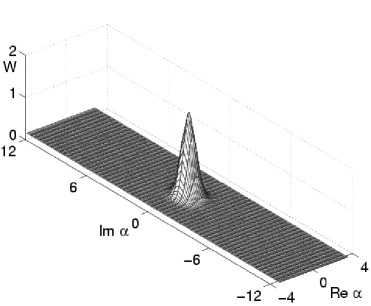
(b)

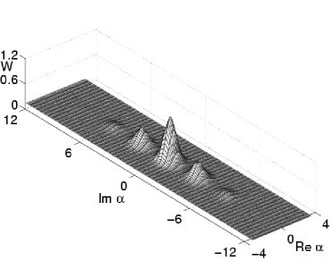
(c)

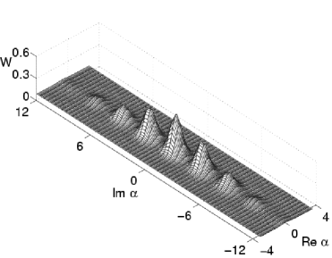
(d)

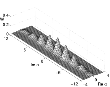
Figure 5: Generation of multi-peaked distributions in the transient cavity field dynamics: $W(\alpha,t)$ distributions at $t=0$ (top) and $\gamma t=0.1,0.3,0.5$ (proceeding downward), obtained from the master equation (21).

All these intertwined tools allow a consistent description of SDM dynamics which complements the analytical results and unveils additional features. As an example, in Fig. 5 we show the transient behavior of the Wigner distribution $W(\alpha)$ of the SDM field. Starting from the Gaussian function of the vacuum state (Fig. 5a), after a time interval $\gamma t=0.1$ (Fig. 5b) we see the presence of two additional peaks, symmetrically placed along the imaginary axis. Here, we have chosen $|\xi|=\pi$, a large enough value to see a peaked structure. At later times in the transition, Fig. 5(c,d), we see the onset of other peak pairs symmetrically placed on the imaginary axis, while the distribution lowers and broadens along that axis. The underlying physical mechanism for the generation of this dynamics was described in Sec. II.

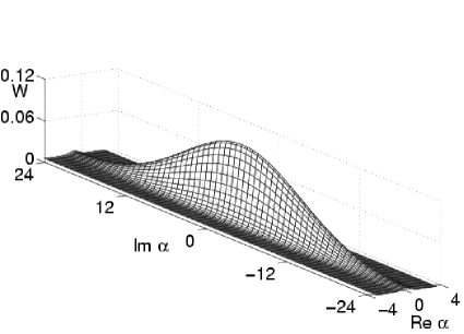
Figure 6: Steady-state cavity field after the transient evolution of Fig. 5: $W(\alpha)$ function at $\gamma t=20$.

At later times decoherence destroys such structures, and when the steady-state is reached (Fig. 6) the distribution looks like the envelope of the multiply-peaked structure along the imaginary axis, while it preserves its initial minimum width along the real axis. Figure 7 shows the density matrix of the steady-state SDM field. The diagonal elements provide the photon statistics, and their wide distribution confirms the predicted super-poissonian behavior. Furthermore, we note the presence of off-diagonal density matrix elements or coherences, which rule the phase and spectral properties of the field.

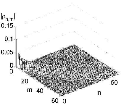
Figure 7: Density matrix of the steady-state cavity field.

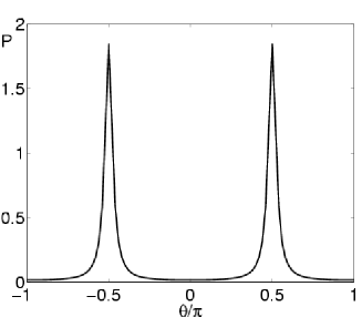
Figure 8: Pegg-Barnett phase distribution of the steady-state cavity field.

Initially they are not excited in the cavity field, hence they are induced by the interaction with the strongly driven atoms. In order to investigate this effect, in Fig. 8, we show the steady-state Pegg-Barnett PB phase distribution

$$P(\theta)=(2\pi)^{-1}\sum_{m,n=0}^{\infty}{\rho_{F}}^{\mathrm{(ss)}}_{n,m}e^{i(m-n)\theta}\,.$$ (41)

The SDM phase distribution shows a particular feature, i.e., a narrow two-peaked structure centered on the values $\theta=\pm\pi/2$, which is already present in the transient. This feature is explained by the SDM gain dynamics, Eq. (19), which shows that the resonant interaction of the cavity field with strongly driven atoms implies an equal displacement of the field by the imaginary quantities $\pm\xi$. In turn, this effect is quite consistent with the narrow elongated form of the steady-state distribution along the imaginary axis in phase space, as well as with the vanishing of the steady-state field expectation value.

V Conclusions

We have investigated the dynamics of a strongly-driven micromaser, based on the resonant interaction of one mode of a high-Q cavity with a poissonian low density beam of two-level atoms strongly driven by a resonant classical field. We have shown that this system provides a nontrivial example of an open quantum system that can be described analytically, exhibiting classical and nonclassical regimes and properties. We have presented the time-dependent solution of the master equation and the expressions of the main statistical quantities for both the cavity field and the detected atoms. In particular, we have found that the steady-state of the SDM photon statistics is always super-poissonian, contrary to the conventional micromaser. On the other hand, atom-atom correlations exhibit stronger nonclassical features than in the micromaser dynamics, due to the stronger entangling nature of the unitary atom-field interaction. We have shown that, in the strong coupling regime, superpositions of coherent states can be generated in the transient dynamics, whose coherence vanishes towards its superpoissonian steady-state. Also, we have shown the two-peaked structure of the SDM Pegg-Barnett phase, explained by the underlying coherent gain mechanism. The SDM model appears quite promising both as a nice theoretical tool, with unusual access to exact analytical developments, and in view of physical implementations, in cavity QED or in the optical regime with high finesse Fabry-Perot cavities m.l. .

VI Acknowledgments

P. L. acknowledges financial support from the Bayerisches Staatsministerium für Wissenschaft, Forschung und Kunst in the frame of the Information Highway Project and E. S. from the EU through the RESQ (Resources for Quantum Information) project.

References

- (1) D. Meschede, H. Walther, and G. Müller, Phys. Rev. Lett. 54, 551 (1985); G. Rempe, H. Walther, and N. Klein, Phys. Rev. Lett. 58, 353 (1987).
- (2) G. Raithel et al. in Advances in Atomic, Molecular and Optical Physics, edited by P.R. Berman (Academic, New York, 1994).
- (3) E.T.Jaynes and F.W. Cummings, Proc. IEEE 51, 89 (1963).
- (4) G. Rempe, F. Schmidt-Kaler, and H. Walther, Phys. Rev. Lett. 64, 2783 (1990).
- (5) M. Weidinger, B. Varcoe, R. Heerlein, and H. Walther, Phys. Rev. Lett. 82, 3795 (1999).
- (6) B. Varcoe, S. Brattke, M. Weidinger, and H. Walther, Nature (London)403, 743 (2000); S. Brattke, B. Varcoe, and H. Walther, Phys. Rev. Lett. 86, 3534 (2001).
- (7) B.-G. Englert, M. Löffler, O. Benson, B. Varcoe, M. Weidinger, and H. Walther, Fortschr. Phys. 46, 897 (1998).
- (8) E. Solano, G. S. Agarwal, and H. Walther, Phys. Rev. Lett. 90, 027903 (2003).
- (9) J.M. Raimond, M. Brune, and S. Haroche, Rev. Mod. Phys. 73, 565 (2001).
- (10) F. Casagrande, A. Lulli, and V. Santagostino, Phys. Rev. A65 023809 (2002); F. Casagrande and A. Lulli, J. Opt. B: Quantum Semiclass. Opt. 4 S260 (2002).
- (11) E. Solano, R. L. de Matos Filho, and N. Zagury, Phys. Rev. Lett. 87 060402 (2001).
- (12) K. E. Cahill and R. J. Glauber, Phys. Rev. 177, 1857 (1969); ibid., 1882 (1969).
- (13) M. Brune, E. Hagley, J. Dreyer, X. Maitre, A. Maali, C. Wunderlich, J.M. Raimond, and S. Haroche, Phys. Rev. Lett. 77, 4887 (1996).
- (14) See, for example, M. O. Scully and M. S. Zubairy, Quantum optics (Cambridge University Press, 1997).
- (15) P. Filipowicz, J. Javanainen, and P. Meystre, Phys. Rev. A34, 3077 (1986); L.A. Lugiato, M.O. Scully, and H. Walther, Phys. Rev. A36, 740 (1987).
- (16) H.-J. Briegel, B.-G. Englert, N. Sterpi, and H. Walther, Phys. Rev. A49, 2962 (1996).
- (17) J. Dalibard, Y. Castin, and K. Mølmer, Phys. Rev. Lett. 68, 580 (1992).
- (18) For a recent application in the study of the micromaser spectrum, see F. Casagrande, A. Ferraro, A. Lulli, R. Bonifacio, E. Solano, and H. Walther, Phys. Rev. Lett. 90, 183601 (2003).
- (19) D.T. Pegg and S.M. Barnett, Phys. Rev. A39, 1665 (1989).
- (20) K. An, J.J. Childs, R.R. Desari, and M. Feld, Phys. Rev. Lett. 73, 3375 (1994).