Coherent states for exactly solvable potentials

Abstract

A general algebraic procedure for constructing coherent states of a wide class of exactly solvable potentials e.g., Morse and Pöschl-Teller, is given. The method, a priori, is potential independent and connects with earlier developed ones, including the oscillator based approaches for coherent states and their generalizations. This approach can be straightforwardly extended to construct more general coherent states for the quantum mechanical potential problems, like the nonlinear coherent states for the oscillators. The time evolution properties of some of these coherent states, show revival and fractional revival, as manifested in the autocorrelation functions, as well as, in the quantum carpet structures.

I Introduction

Coherent states (CS) and their generalizations, in the context of harmonic oscillators, are well-studied in the literature glauber ; klauder2 ; perelomov ; gilmore . Algebraic approaches have been particularly useful for providing a unified treatment of these states and their inter-relationships. For example, in Ref. shanta , not only a general procedure for constructing a large class of oscillator based CS has been provided, but it has also been shown that, some of these states are dual to each other in a well-defined manner. The algebraic approaches straightforwardly lead to the construction of squeezed and other states showing interesting non-classical features. These elegant and powerful algebraic procedures of construction owe their origin, partly, to the simplicity of the Heisenberg-Weyl algebra; $[a,a^{\dagger}]=1$, characterizing the harmonic oscillator. Based on the symmetries and keeping in mind the desired requirements, various procedures have been developed for constructing CS for Morse benedict ; roy ; fakhri ; nietoprd3 , Hydrogen atom gerry , Pöschl-Teller nietoprd2 ; crawford ; klauder3 ; kinani and other potentials mohanty . The role of Morse potential in molecular physics is well-known child . The study of CS for hydrogenic atoms have assumed increasing importance in light of their relevance to Rydberg states stroud , which may find potential application for quantum information processing rangan .

It is known that, all the criteria desired of a coherent state and found in the oscillator based CS, e.g., minimum uncertainty product, eigenstate of the annihilation operator (AO) and displacement operator states are not simultaneously achievable in other potential based CS. Hence, a number of CS, diluting one or more of the above criteria, have been constructed in the literature.

In the context of algebraic approaches, supersymmetric (SUSY) quantum mechanics khare based raising and lowering operators have found significant application. In particular, eigenstates of the lowering operator for Morse benedict and Pöschl-Teller kinani potentials have been found and their properties studied. Recently Antoine et. al. klauder3 have constructed Klauder type CS for the Pöschl-Teller potential, using a matrix realization of ladder operators, their motivation being the temporal stability of the CS. It is well-known that the SUSY ladder operators act on the Hilbert space of different Hamiltonians except for the case of the harmonic oscillator. Establishing a precise connection between the complete set of states, describing the above CS, and the symmetries of these potential problems has faced difficulties fakhri ; jellal . To be specific, in case of the Barut-Girardello CS for the Morse potential, the ladder operators are taken to be functions of quantum numbers, which has led to problems in defining a proper algebraic structure. To resolve the same, some authors fakhri have resorted to the introduction of additional angular coordinates asim .

In this work, we provide an algebraic construction of the CS for a wide class of potentials, belonging to the confluent hypergeometric (CHG) and hypergeometric (HG) classes. The procedure is based on a simple method of solving linear differential equations (DEs) guru1 , which enables one to express the solutions in terms of monomials. In the space of monomials, it is straightforward to identify various types of ladder operators, their underlying algebraic structures guru2 , and construct lowering operator eigenstate in a transparent manner. The fact that, the monomials and the quantum mechanical eigenfunctions are connected through similarity transformations, enables one to preserve these algebraic structures at the level of the wavefunctions and simultaneously obtain the desired CS. Thus the coherent state is initially potential independent. The information about a specific potential is then incorporated by fixing the parameters of the series and also the ground state wavefunction of the potential under study. The known results for CS are obtained in specific limits. In addition, our procedure demonstrates the construction of more general CS, similar to the nonlinear CS sudarshan in the oscillator example. The origin of confusion in identifying the algebraic structure in SUSY based approaches is then pointed out and subsequently resolved in a natural manner. It is shown that the recently found CS for various potentials are related to the two different realizations of SU(1,1) algebra.

The paper is organized as follows. Keeping in mind the connection of the wavefunctions of the exactly solvable potentials, to be considered here, and the solutions of the CHG and HG DEs, we first briefly outline the relationship between the solutions of the above equations and the space of monomials. This connection is then made use of, to identify the ladder operators and the symmetry algebras in the space of monomials. AOCS are constructed, through a recently proposed procedure for solving linear DEs. This method yields the precise connection between the present, and the earlier oscillator based approaches for constructing CS. In Sec. III, the potential independent CS, thus constructed, are connected with Morse and Pöschl-Teller potentials, as examples. The advantage of constructing the ladder operators in the space of monomials is then pointed out by resolving the difficulties in identifying the symmetry generators in the SUSY based approach. Various earlier known CS are then derived as special cases. Time evolution properties of some of these CS are then studied. Autocorrelation functions and the underlying quantum carpet structures frank of these CS clearly reveal the phenomena of revival and fractional revival banerji . We conclude in Sec. IV after pointing out a number of open interesting problems, where the present procedure can be profitably employed. Keeping in mind the rich symmetry structure of the hydrogen atom problem and the various procedures employed for constructing the corresponding CS, we desist from the analysis of these CS here; this will be taken up in a future project.

II Algebraic construction of coherent states

This section is devoted to the construction of CS in a manner which is potential independent. We make essential use of the fact that the exactly solvable potentials, to be studied here, belong to the CHG and the HG classes, whose solutions can be connected to the space of monomials through similarity transformations. In the space of monomials, the identification of symmetry algebras and their ladder operators become easy. The AO eigenstates in the space of monomials are first found through the above mentioned procedure of solving DEs and then connected to those at the level of the polynomials, through similarity transformation. Connection with earlier oscillator based approaches is also exhibited.

A single variable linear DE, of arbitrary order, can be cast in the form $[F(D)+P(x,d/dx)]y(x)=0$; where $F(D)$ is a function of the Euler operator $D=xd/dx$ and $P(x,d/dx)$ contains rest of the operators. A formal series solution of the above DE is given by guru1 ; guru2

$$y(x)=C_{\alpha}\sum_{n=0}^{\infty}(-1)^{n}\left[\frac{1}{F(D)}P(x,d/dx)\right]^{n}x^{\alpha}\,,$$ (1)

provided the condition $F(D)x^{\alpha}=0$, is satisfied. This condition fixes the value of $\alpha$. Here $C_{\alpha}$ is the normalization constant. The proof is straightforward and follows by direct substitution. In the CHG and the HG cases, $\alpha=n$ (integer) corresponds to polynomial solutions and for $\alpha\neq n$ series solutions are obtained.

Following an earlier work guru2 , the simplest set of operators, at the level of monomials, which give rise to a SU(1,1) algebra can be written as brif

$$K_{+}=x,K_{-}=\left[x\frac{d^{2}}{dx^{2}}+b\frac{d}{dx}\right],\,{\rm and}\,K_{3}=\left[x\frac{d}{dx}+\frac{b}{2}\right].$$ (2)

Here $b$ is deliberately taken same as the CHGDE parameter, so that the algebra is well defined at the level of the wavefunctions. It should be noted that, these symmetry algebras are not unique, and the interesting consequences arising from this fact will be pointed out later. The AOCS corresponding to $K_{-}$ satisfies,

$$K_{-}\varphi(x,\beta)=-\beta\varphi(x,\beta)\,.$$ (3)

Left multiplying by $x$:

$$\left(x^{2}\frac{d^{2}}{dx^{2}}+bx\frac{d}{dx}+\beta x\right)\varphi(x,\beta)=0\,$$ (4)

one can identify $F(D)=(D+b-1)D$ and $P(x,d/dx)=\beta x$. The condition $F(D)x^{\alpha}=0$ gives $\alpha=0,1-b$. For $\alpha=0$ one obtains,

$$\varphi(x,\beta) = N(\beta)^{-1}\sum_{n=0}^{\infty}(-1)^{n}\left[\frac{\beta}{(D+b-1)D}x\right]^{n}x^{0}\,,$$ (5)

$$= N(\beta)^{-1}\sum_{n=0}^{\infty}\frac{(-1)^{n}}{n!}\frac{(\beta x)^{n}}{(b)_{n}}\,=\exp\left[-\frac{\beta}{(D+b-1)}x\right]\,.$$

$N(\beta)^{-1}$ is the normalization constant. The commutation relation, $[D,x^{d}]=dx^{d}$, and the definition of the Pochhammer’s symbol, $(b+n-1)\cdots b=\Gamma(b+n)/\Gamma(b)=(b)_{n}$, have been used in the above derivation. We can make immediate contact with the oscillator based approach of Ref. shanta . Denoting

$$\tilde{K}_{+}\equiv\frac{1}{(D+\beta-1)}x\,,$$ (6)

it is found that, they obey the Heisengerg-Weyl algebra, $[K_{-},\tilde{K}_{+}]=1$. Such conjugate operators were explicitly constructed in shanta and used to obtain a large class of multi-photon coherent states.

Knowing that the solution of the CHGDE can be written in the form guru1

$$\Phi(-n;b;x)=(-1)^{n}\frac{\Gamma(b)}{\Gamma(b+n)}e^{-K_{-}}x^{n}\,,$$ (7)

one can obtain the coherent state at the level of the polynomial and later on at the level of the wavefunctions through appropriate similarity transformations, as illustrated below. Denoting $S\equiv\exp(-K_{-})$, one obtains $SK_{-}S^{-1}S\varphi(x,\beta)=\beta S\varphi(x,\beta)=\beta\tilde{\varphi}(x,\beta)$, where $\tilde{\varphi}(x,\beta)$ is the coherent state at the level of the polynomial:

$$\tilde{\varphi}(x,\beta)=N(\beta)^{-1}\sum_{n=0}^{\infty}\frac{\beta^{n}}{n!}\Phi(-n;b;x)\,.$$ (8)

It will be seen explicitly in the subsequent section that introducing appropriate measures through similarity transformations one would obtain CS for various quantum mechanical systems. It is worth emphasizing that the algebraic structures are transparently preserved in this approach.

Analogously for HG case, taking the lowering operator to be guru2

$$\hat{K}_{-}=\frac{1}{(D+b)}\left(x\frac{d^{2}}{dx^{2}}+c\frac{d}{dx}\right)\,,$$ (9)

the coherent state at the level of polynomials is given by

$$\tilde{\chi}(x,\gamma)=N(\gamma)^{-1}\sum_{n=0}^{\infty}\frac{\gamma^{n}}{n!}{{}_{2}}F_{1}(-n,b;c;x)\,,$$ (10)

since

$$_{2}F_{1}(-n,b;c;x)=(-1)^{n}\frac{\Gamma(b+n)\Gamma(c)}{\Gamma(c+n)\Gamma(b)}e^{-\hat{K}_{-}}x^{n}\,.$$ (11)

We can connect to the oscillator based approach in this case also; calling

$$\bar{K}_{+}\equiv\frac{(D+b-1)}{(D+c-1)}x\,,$$ (12)

it satisfies the oscillator algebra: $[{\hat{K}}_{-},\bar{K}_{+}]=1$. It should be noted that the states obtained using the lowering operator ${\hat{K}}_{-}$ are nonlinear CS sudarshan . They are defined to be eigenstates of the AO of the type $f({\mathcal{N}})T_{-}$, $f({\mathcal{N}})$ being a function of the number operator in the oscillator case and the Euler operator in the present one; $T_{-}$ is an arbitrary lowering operator. It was recently shown wang that, the AOCS and the Perelomov CS are unified in the framework of nonlinear CS.

Equations (8) and (10) reveal that these CS are quite general; since the eigenfunctions of the exactly solvable potentials to be considered here, arise as special cases of CHG and HG series, their corresponding CS will also follow from the above two general expressions. In fact, starting from the lowering operator

$${\tilde{T}}_{-}=\frac{(D+b_{1})\cdots(D+b_{p})}{(D+a_{1})\cdots(D+a_{p})}\frac{d}{dx}\,;$$ (13)

more general nonlinear CS can be found:

$$\xi(x,\alpha)=\sum_{n=0}^{\infty}\frac{\alpha^{n}}{n!}{{}_{p+1}}F_{p}(a_{1},\cdots,a_{p},-n;b_{1},\cdots,b_{p};x).$$ (14)

Here ${{}_{p+1}}F_{p}$ is the generalized HG series. For the sake of completeness it should be pointed out, the above summation yields bateman

$$\xi(x,\alpha)={{}_{p}}F_{p}(a_{1},\cdots,a_{p};b_{1},\cdots,b_{p};-x\alpha)e^{\alpha}.$$ (15)

It is worth noting that the weight factors associated with the above CS, play an important role in the study of photon number statistics in quantum optics, where similar type of states also appear appl .

III Connection with potentials

We now proceed to specific potentials for the purpose of illustration and establishing connections with the various CS obtained so far. We use the Morse potential benedict ; roy ; fakhri ; nietoprd3 as an example, for the CHG class of potentials, and the Pöschl-Teller (PT) potential nietoprd2 ; crawford ; klauder3 ; kinani for the HG class.

The one dimensional Morse potential is given by

$$V_{\rm M}=d[1-\exp(-ay)]^{2},$$ (16)

$a$ and $d$ (depth of the potential) being constant parameters. Introducing dimensionless parameter $\mu=\sqrt{2md}/a\hbar$, dimensionless coordinate $q=ay$ and using the transformation rule: $x=2\mu\exp(-q)$; the Schrödinger equation yields the eigenfunction

$$\psi^{\rm M}_{n}(x)\propto e^{-x/2}x^{\lambda/2}L_{n}^{\lambda}(x)\,,$$ (17)

where we have set $\lambda=2\mu-2n-1$ for the sake of convenience. Multiplying Eq. (8) from the left, by the ground state of the Morse eigenstate: $\psi^{\rm M}_{0}(x)\equiv\exp(-x/2)x^{\lambda/2}$, and noting that, for $b=\lambda+1$ the CHG series can be expressed in terms of the Laguerre polynomials stegun

$$\Phi(-n;\lambda+1;x)=\frac{n!}{(\lambda+1)_{n}}L_{n}^{\lambda}(x)\,;$$ (18)

the coherent state for the Morse potential can be written from the results of the previous section:

$${\tilde{\varphi}}_{\rm M}(x,\beta)=N(\beta)^{-1}\Gamma(\lambda+1)\psi^{\rm M}_{0}\sum_{n=0}^{\infty}\frac{\beta^{n}L_{n}^{\lambda}(x)}{\Gamma(\lambda+n+1)}.$$ (19)

After normalization one finds,

$${\tilde{\varphi}}_{\rm M}(x,\beta) = \frac{|\beta|^{\lambda/2}}{\sqrt{I_{\lambda}(2|x|)}}\sum_{n=0}^{\infty}\frac{\beta^{n}}{\Gamma(\lambda+n+1)}\psi^{\rm M}_{n}(x)$$ (20)

$$= \frac{|\beta|^{\lambda/2}}{\sqrt{I_{\lambda}(2|x|)}}(\beta)^{-\lambda/2}e^{\beta}e^{-x/2}J_{\lambda}(2\sqrt{x\beta})\,.$$

Here, $I_{\lambda}$ is the modified Bessel function of the first kind and $J_{\lambda}$ is the Bessel function of the first kind. The same expression was obtained in jellal using the SUSY based ladder operators.

In order to see the difficulties associated with properly defining an algebraic structure using SUSY based ladder operators jellal

$$A^{\pm}\psi^{\rm M}_{n}(x)=\left[x\frac{d}{dx}\pm\frac{1}{2}(2n+\lambda+1-x)\right],$$ (21)

as alluded to earlier, we explicitly write down the action of the same on the wavefunctions: $A^{+}\psi^{\rm M}_{n}(x)=\sqrt{(n+1)(n+\lambda+1)}\psi^{\rm M}_{n+1}(x)$ and $A^{-}\psi^{\rm M}_{n}(x)=-\sqrt{n(n+\lambda)}\psi^{\rm M}_{n}(x)$. In earlier works without explicitly giving the diagonal operator, its action was inferred from $[A^{+},A^{-}]\psi^{\rm M}_{n}(x)$. However, as was noticed in fakhri this approach faces problem in constructing the Barut-Girardello CS. To better appreciate the difficulties and its resolution, we first identify the corresponding ladder operators at the level of monomials through similarity transformations, which keeps the algebraic structure intact. These operators act as

$$(K_{+}+D-n)x^{n}=x^{n+1}\quad(K_{-}+D-n)x^{n}=n(n+\alpha)x^{n-1}.$$ (22)

It can be noticed that as compared to our ladder operators, at the level of monomials, the above ones contain an additional operator $D-n$, which yields zero when acting on monomial $x^{n}$. It can be straightforwardly seen that the SUSY based $n$ dependent operators do not lead to a proper algebra, a difficulty noticed in fakhri . However, the $n$ independent operators lead to the diagonal operator $K_{3}=xd/dx+b/2$; together these form a closed SU(1,1) algebra. Hence, for the construction of AOCS with a well defined algebraic structure, it is imperative to use $n$ independent operators. It can be seen that for the ground state, from which the AOCS are constructed, the above $n$ dependent operator is absent. Hence the expression for the CS derived earlier jellal and the one obtained here, based on the SU(1,1) algebra, are identical.

As mentioned earlier the SU(1,1) generators written above are not unique e.g., the following three generators also form a SU(1,1) algebra perelomov :

$$L_{+}=x^{2}\frac{d}{dx}+2(\lambda+1)x,\quad L_{-}=\frac{d}{dx},\quad{\rm and}\quad L_{3}=x\frac{d}{dx}+\frac{(\lambda+1)}{2}.$$ (23)

The eigenstate of $L_{-}$ is given by $\exp(\beta x)$. The corresponding AOCS, at the level of the wavefunction for the Morse potential, can be obtained by making use of the following identities,

$$\exp\left[-x\frac{d^{2}}{dx^{2}}-(\lambda+2)\frac{d}{dx}\right].\frac{d}{dx}=\frac{d}{dx}.\exp\left[-x\frac{d^{2}}{dx^{2}}-(\lambda+1)\frac{d}{dx}\right]$$ (24)

and

$$\exp\left[-x\frac{d^{2}}{dx^{2}}-(\lambda+1)\frac{d}{dx}\right]\exp(\beta x)=\sum_{n=0}^{\infty}\beta^{n}L_{n}^{\lambda}(x).$$ (25)

The resulting coherent state turns out to be the Perelomov coherent state for this potential benedict :

$${\tilde{\varphi}}^{\rm PER}_{\rm M}(x,\beta)=\frac{(1-|\beta|^{2})^{(\lambda+1)/2}}{\sqrt{\Gamma(\lambda+1)}}x^{\lambda/2}\exp\left(-\frac{x}{2}\frac{1+\beta}{1-\beta}\right)\,.$$ (26)

Hence, the above SU(1,1) algebra gives the operator, whose eigenstate is the Perelomov coherent state; recourse has been taken earlier to more complicated nonlinear algebras for this purpose wang .

We now derive the CS for the PT class of potentials and concentrate primarily on the symmetric PT (SPT) and PT potentials. Plots of the weight factors associated with the CS of the above mentioned potentials will be given along with the quantum carpet structure and the auto-correlation figures. The quantum carpet and the autocorrelation plots, transparently bring out the phenomenon of revival and fractional revival.

The SPT potential is

$$V_{\rm SPT}(y)=\frac{\hbar^{2}\alpha^{2}}{2m}\frac{\rho(\rho-1)}{\cos^{2}\alpha y}$$ (27)

and the corresponding eigenvalues and eigenfunctions, in the variable $x=\sin\alpha y$, are

$$E^{\rm SPT}_{n} = \frac{\hbar^{2}\alpha^{2}}{2m}(n+\rho)^{2},\quad n=0,1,2,\cdots$$

$$\psi_{n}^{\rm SPT}(x) = \left[\frac{\alpha(n!)(n+\rho)\Gamma(\rho)\Gamma(2\rho)}{\sqrt{\pi}\Gamma(\rho+1/2)\Gamma(n+2\rho)}\right]^{1/2}(1-x^{2})^{\rho/2}C_{n}^{\rho}(x)\,.$$ (28)

The Gegenbauer polynomials are related to the HG series via the relation stegun

$${{}_{2}}F_{1}(-n,n+2\rho;\rho+1/2;z)=\frac{n!}{(2\rho)_{n}}C_{n}^{\rho}(1-2z)\,.$$ (29)

Multiplying $(1-x^{2})^{\rho/2}$ from the left in Eq. (10) and using Eqs. (28) and (29), the coherent state for the SPT potential is found to be

$$\tilde{\chi}_{\rm SPT}(x,\gamma)=N(\gamma)^{-1}\sum_{n=0}^{\infty}\left[\frac{\Gamma(2\rho)\Gamma(\rho+1/2)\sqrt{\pi}}{\alpha(n!)(n+\rho)\Gamma(\rho)\Gamma(2\rho+n)}\right]^{1/2}\gamma^{n}\psi_{n}^{\rm SPT}(x)\,.$$ (30)

The normalization constant, $N(\gamma)^{-1}$, is

$$N(\gamma)^{-1}=\left[\frac{\alpha\Gamma(\rho)}{\Gamma(\rho+1/2)\Gamma(2\rho)\sqrt{\pi}S(|\gamma|)}\right]^{1/2}$$

where,

$$S(|\gamma|)=\sum_{n=0}^{\infty}\frac{|\gamma|^{2n}}{n!(n+\rho)\Gamma(2\rho+n)}=\frac{1}{|\gamma|^{2\rho}}\int^{2|\gamma|}_{0}dxI_{2\rho-1}(x)\,.$$ (31)

It is worth pointing out that the CS for the SPT potential can be expressed in terms of the Bessel functions by using a generating function of the Gegenbauer polynomials stegun :

$$\tilde{\chi}_{\rm MPT}(x,\gamma)=N(\gamma)^{-1}\Gamma(\rho+1/2)e^{\gamma x}\left(\frac{\gamma}{2}\right)^{1/2-\rho}J_{\rho-1/2}(\gamma\sqrt{1-x^{2}}).$$ (32)

Similarly we can construct the CS for the PT potential. The PT potential is

$$V_{\rm PT}(x)=\frac{\hbar^{2}\alpha^{2}}{2m}\left[\frac{\kappa(\kappa-1)}{\sin^{2}\alpha x}+\frac{\rho(\rho-1)}{\cos^{2}\alpha x}\right],\quad\kappa,\rho>1\,,$$ (33)

whose energy eigenvalues and the eigenfunctions are

$$E_{n}^{\rm PT} = \frac{\hbar^{2}\alpha^{2}}{2m}(\kappa+\rho+2n)^{2},\quad n=0,1,2,\cdots$$

$$\psi_{n}^{\rm PT}(x) = C_{n}(\cos\alpha x)^{\lambda}(\sin\alpha x)^{\kappa}P_{n}^{(\kappa-1/2,\rho-1/2)}(1-2\sin^{2}\alpha x)$$ (34)

Here $C_{n}$ is the normalization constant and given by normalization

$$C_{n}=\left[\frac{2\alpha(\kappa+\rho+2n)\Gamma(n+1)\Gamma(\kappa+\rho+n)}{\Gamma(\kappa+n+1/2)\Gamma(\rho+n+1/2)}\right]^{1/2}\,.$$ (35)

Using Eq. (34) and Eq. (35) in Eq. (10) the AOCS for the Pöschl-Teller potential can be written in the form

$${\tilde{\chi}}_{\rm PT}(x,\gamma)=N(\gamma)^{-1}\sum_{n=0}^{\infty}\gamma^{n}\left[\frac{\Gamma(\kappa+1/2)(\lambda+1/2)_{n}}{2\alpha(\kappa+1/2)_{n}(\kappa+\rho+2n)\Gamma(n+1)\Gamma(\kappa+\rho+n)}\right]^{1/2}\psi_{n}^{\rm PT}(x)\,.$$ (36)

In the above equation relation between Jacobi polynomials and HG series has been used stegun . As has been done for the Morse potential one can also construct Perelomov type coherent state here.

The quadratic nature of the eigenspectra of PT and SPT lead to the possibility of revival and fractional revival in this quantum system. Keeping this in mind, we now proceed to study the time evolution property of the above CS. As expected, these states show a very rich structure involving revival and fractional revivals. We give in Fig (1) quantum carpet representing the time evolution of the above state. The plots for the auto correlation are provided Figs (3) and (4), which clearly bring out the above features. Interestingly, there have been some recent proposals to use the fractional revival for the purpose of factorization of numbers mack . In the above quantum carpet the ridges and the valleys follow a curved path, unlike the square-well case where these are straight lines frank . We also notice richer structure arising due to interference. The origin of these structures in the square-well case have been understood, the present scenario needs a thorough understanding.

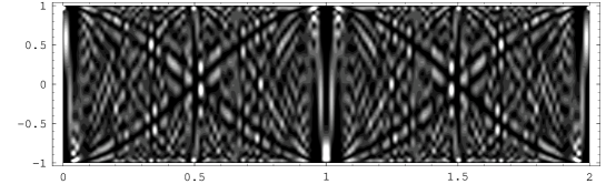
Figure 1: The density plot of $|\tilde{\varphi}(x,t)|^{2}$ for, $\gamma=10$ and the maximum value of $n=20$ in the symmetric Pöschl-Teller potential. Darkness displays a low and brightness a high functional value.

Figure 2: Squared modulus $\mid_{\rm SPT}\langle x,\gamma,t\neq 0\mid x,\gamma,t=0\rangle_{\rm SPT}\mid^{2}$ ($y$-axis) and time ($x$-axis), for $\gamma=10$, $\rho=2$, and $n=20$, of the autocorrelation for the SPT potential. The peaks show the revivals whereas the intermediate ones fractional revivals

Figure 3: Squared modulus $\mid_{\rm PT}\langle x,\gamma,t\neq 0\mid x,\gamma,t=0\rangle_{\rm PT}\mid^{2}$ ($y$-axis) and time ($x$-axis), for $\gamma=10$, $\kappa=2$, $\rho=6$, and $n=20$, of the autocorrelation for the PT potential.

As is well-known, the weight factors associated with the CS carry physical significance e.g., these factors for the oscillator CS give rise to a Poisson distribution. The weight factors associated with the HG class of CS, derived above, are related to the HG distribution in probability theory feller , as is clear from the plot of the weighting distribution in Fig (5).

Figure 4: Plot of the weighting distribution $|c_{n}|^{2}$ ($y$-axis) in Eq. (30), with respect to $n$ ($x$-axis). This plot captures the HG statistical nature of the coherent state. Here $\gamma=10$, $\rho=2$, and the maximum value of $n$ is 20.

IV Conclusions

In conclusion, we have developed a general algebraic procedure for finding the annihilation operator coherent states for a wide class of quantum mechanical potentials. Interestingly, the Perelomov type CS also emerged, as AOCS, from different realizations of relevant symmetry algebras. Crucial use was made of a simple method for solving linear DEs, which gives a precise connection between the solution space and the space of monomials. Ladder operators, corresponding to various symmetry algebras can be identified straightforwardly. The method is potential independent and enables one to find the AOCS and connect them with earlier oscillator based approaches. It is applicable to quantum problems having infinite number of bound states as well as the ones possessing finite numbers. Generalizations to analogs of the nonlinear CS for oscillators is also made transparent.

Under time evolution, these CS showed revival and fractional revivals. This manifests in the quantum carpet structure as well as the auto-correlation functions. Interestingly, these phenomena in the context of square-well frank have led to a proposal for factorizing numbers mack . The intricate structure of quantum carpet needs careful analysis in light of recent proposals to use CS for quantum information storage enk . The weighting distributions associated with these CS also needs to be studied more elaborately, in the complete parameter range, for manifestation of non-classical behavior.

Also as a continuation of the present work, it would be interesting to study the features of Wigner quasi-probability distributions for these CS, in light of the interesting results obtained recently in this area zurek . It is worth noting that, recently the Wigner distribution for the Morse eigenstates have been studied wolf . Since the method used here also applies to many-body interacting systems it is worth constructing and studying the corresponding CS chaturvedi . A number of these questions are currently under study and will be reported elsewhere.

References

- (1) J.R. Klauder, Ann. Phys. 11, 123 (1960); R.J. Glauber, Phys. Rev. Lett. 10 84 (1963); E.C.G. Sudarshan, ibid. 10, 277 (1963); J.R. Klauder, J. Math. Phys. 4, 1055 (1963); A.O. Barut and L. Girardello, Commun. Math. Phys. 21, 41 (1971); M.M. Nieto and L.M. Simmons, Jr., Phys. Rev. Lett. 41, 207 (1978); J.P. Gazeau and J.R. Kaluder, J. Phys. A 32, 123 (1999).
- (2) J.R. Klauder and B.S. Skagerstam, Coherent States-Applications in Physics and Mathematical Physics, World Scientific, Singapore (1985).
- (3) A.M. Perelomov, Generalized Coherent States and Their Application, Springer, Berlin (1986).
- (4) W.M. Zhang, D.H. Feng, and R. Gilmore, Rev. Mod. Phys. 62, 867 (1990) and references therein.
- (5) P. Shanta, S. Chaturvedi, V. Srinivasan, G.S. Agarwal, and C.L. Mehta, Phys. Rev. Lett. 72, 1447 (1994).
- (6) M.G. Benedict and B. Molnár, Phys. Rev. A 60, R1737 (1999).
- (7) B. Roy and P. Roy, Phys. Lett. A 296, 187 (2002).
- (8) H. Fakhri and A. Chenaghlou, Phys. Lett. A 310, 1 (2003).
- (9) M.M. Nieto and L.M. Simmons, Jr., Phys. Rev. D 20, 1342 (1979).
- (10) C.C. Gerry and J. Kiefer, Phys. Rev. A 37, 665 (1988); J.R. Klauder, J. Phys. A 29, L293 (1996); P. Majumdar and H.S. Sharatchandra, Phys. Rev. A 56, R3322 (1997); R.F. Fox, ibid. 59, 3241 (1999); M.G.A. Crawford, ibid. 62, 12104 (2000); S.A. Polshin, J. Phys. A 33, L357 (2000) and references therein.
- (11) M.M. Nieto and L.M. Simmons, Jr., Phys. Rev. D 20, 1332 (1979).
- (12) M.G.A. Crawford and E.R. Vrscay, Phys. Rev. A 57, 106 (1998).
- (13) J.P. Antoine, J.P. Gazeau, J.R. Klauder, P. Monceau, and K.A. Penson, J. Math. Phys. 42, 2349 (1999) and references therein.
- (14) A.H. Kinani and M. Daoud, Phys. Lett. A 283, 291 (2001).
- (15) N. Gurappa, P.S. Mohanty, and P.K. Panigrahi, Phy. Rev. A 61, 34703 (2000); M.M. Nieto, Mod. Phys. Lett. A 16, 2305 (2001); A. Chenaghlou and H. Fakhri, ibid. 17, 1701 (2002).
- (16) M.S. Child and L. Halonen, L. Adv. Chem. Phys., 62, 1 (1984); L. Pauling and E.B. Wilson, Jr., Introduction to Quantum Mechanics with Apllications to Chemistry, Dover, New York (1985); P. Jensen, P. Mol. Phys. 98, 1253 (2000) and references therein.
- (17) A. ten Wolde, L.D. Noordam, H.G. Muller, A. Lagendijk, and H.D. van Linden van den Heuvell, Phys. Rev. Lett. 61, 2099 (1988); J.A. Yeazell, M. Mallalieu, J. Parker, and C.R. Stroud, Jr., Phys. Rev. A 40, 5040 (1989); J.A. Yeazell and C.R. Stroud, Jr., ibid. 43, 5153 (1991); E.A. Shapiro and P. Bellomo, ibid. 60, 1403 (1999) and references therein.
- (18) A. Muthukrishnan and C.R. Stroud, Jr., quant-ph/0106165; J. Ahn, C. Rangan, D.N. Hutchinson, and P.H. Bucksbaum, Phys. Rev. A 66, 22312 (2002); M.S. Safronova, C.J. Williams, and C.W. Clark, Phys. Rev. A 67, 40303 (2003) and references therein.
- (19) F. Cooper, A. Khare, and U.P. Sukhatme, Phys. Rep. 251, 268 (1995); F. Cooper, A. Khare, and U.P. Sukhatme, Supersummetry in Quantum Mechanics, World Scientific, Singapore (2001).
- (20) A. Jellal, Mod. Phys. Lett. A 17, 671 (2002).
- (21) A. Gangopadhyaya, J.V. Mallow, and U.P. Sukhatme, Phys. Rev. A 58, 4287 (1998).
- (22) N. Gurappa and P.K. Panigrahi, Phys. Rev. B 62, 1943 (2000); N. Gurappa and P.K. Panigrahi, ibid. 67, 155323 (2003).
- (23) N. Gurappa, P.K. Panigrahi, T. Shreecharan, and S. Sree Ranjani, in Frontiers of Fundamental Physics 4, Eds. B.G. Sidharth and M.V. Altaisky, Kluwer, New York (2001); N. Gurappa, P.K. Panigrahi, and T. Shreecharan to appear in J. Comp. App. Math. (math-ph/0203015).
- (24) R.L. de Filho and W. Vogel, Phys. Rev. A 54, 4560 (1996); V.I. Man’ko, G. Marmo. E.C.G. Sudarshan, and F. Zaccaria, Physica Scripta 55, 528 (1997); O.V. Man’ko, Phys. Lett. A 228, 29 (1997); S. Mancini, ibid. 233, 29 (1997).
- (25) F. Grobmann, J.M. Rost, and W.P. Schleich, J. Phys. A 30, L277 (1997); M.J.W. Hall, M.S. Reineker, and W.P. Schleich, ibid. 32, 8275 (1999).
- (26) I.Sh. Averbukh and N.F. Parleman, Phys. Lett. A 139, 449 (1989); Z.D. Gaeta and C.R. Stroud, Jr., Phys. Rev. A 42, 6308 (1990); R. Bluhm, V.A. Kostelecky, and B. Tudose, ibid. 52, 2234 (1995); G.S. Agarwal and J. Banerji, ibid. 57, 3880 (1998) and references therein.
- (27) C. Brif, Int. J. Theor. Phys. 36, 1651 (1997).
- (28) X.G. Wang, Int. J. Mod. Phys. B 14(10), 1093 (2000).
- (29) A. Erdélyi et. al. Higher Transcendental Functions: Vol III, McGraw-Hill, New York (1955).
- (30) H.C. Fu and R. Sasaki, J. Math. Phys. 38, 2154 (1997); T. Appl and D.H. Schiller, quant-ph/0308013.
- (31) M. Abramowitz and I.A. Stegun, Handbook of Mathematical Functions, Dover Publications, New York (1970).
- (32) M.M. Nieto, Phys. Rev. A 17, 1273 (1978).
- (33) W. Feller, An Introduction to Probability: Theory and Its Applications Vol.1, John-Wiley, New-York (1957).
- (34) H. Mack, M. Bienert, F. Haug, M. Freyberger, and W.P. Schleich, Phys. stat. sol (b) 233, 408 (2002) (quant-ph/020802).
- (35) S.J. van Enk, Phys. Rev. Lett. 91, 17902 (2003); N. Ba An, Phys. Rev. A 68, 22321 (2003) and references therein.
- (36) W.H. Zurek, Nature 412, 712 (2001).
- (37) A. Frank, A.L. Rivera, and K.B. Wolf, Phys. Rev. A 61, 54102 (2000).
- (38) G.S. Agarwal and S. Chaturvedi, J. Phys. A 28, 5747 (1995); B. Sutherland, Phys. Rev. Lett. 80, 3678 (1998).