Adiabatic Time Evolution in Spin-Systems

Abstract

Adiabatic processes in the quantum Ising model and the anisotropic Heisenberg model are discussed. The adiabatic processes are assumed to consist in the slow variation of the strength of the magnetic field that environs the spin-systems. These processes are of current interest in the treatment of cold atoms in optical lattices and in Adiabatic Quantum Computation. We determine the probability that, during an adiabatic passage starting from the ground state, states with higher energy are excited.

I Introduction

The analysis of ground state properties of spin systems in the vicinity of quantum phase transitions is a contemporary issue in statistical physics and condensed matter physics. These systems display a rich variety of phenomena which explain many exotic properties of materials at very low temperature. Very recently, it has been recognized that cold atoms in optical lattices can be very well described in terms of certain spin Hamiltonians Jaksch et al. (1998); Greiner et al. (2002). These systems can be very well controlled at the quantum level, which may allow us to observe physical phenomena predicted for spin systems and that have, so far, not been observed with other systems. Moreover, they may allow to build a quantum simulator which may shed some light in unresolved issues in condensed matter physics Jané et al. (2002).

In the strong interacting regime and at sufficiently low temperature, atoms confined in optical lattices tend to distribute in the so–called Mott phase; that is, under the appropriate conditions each lattice site is occupied by a single atom. Each atom still interacts with the nearest neighbor via virtual tunneling, which gives rise to an effective interaction between the internal levels of neighboring atoms. Under certain conditions, these interactions can be described in terms of the Ising Model or the anisotropic Heisenberg Model with a transverse magnetic field Duan et al. (2002); García-Ripoll and Cirac (2003); Dorner et al. (2003). Changing the laser parameters amounts to varying the parameters of these models. Both models display quantum phase transitions Sachdev (1999) for certain values of these parameters. Thus, with these systems it is possible to investigate the dynamics of quantum phase transitions by, for example, adiabatically changing these laser properties . An important question in this case is to what extent the process can remain adiabatic since near a phase transtion the energy levels tend to get closer as the number of particles increases Dorner et al. (2003). In this paper we will study this problem for both Hamiltonians. For the exactly solvable Ising Model, the adiabatic process will be investigated in detail and analytical results for the excitation probability will be given. For the yet unsolved anisotropic Heisenberg Model, the adiabatic process will be investigated by means of perturbation theory.

Another subject in which the results about adiabatic processes in spin-systems are relevant is Adiabatic Quantum Computation Farhi et al. (2000); Childs et al. (2001); van Dam et al. (2002). In Adiabatic Quantum Computation, solutions to mathematical and physical problems are obtained by simulating adiabatic processes on quantum computers Feynman (1982); Lloyd (1996); Abrams and Lloyd (1997); Wu et al. (2002). An interesting problem related to Adiabatic Quantum Computation is the investigation of the ground state of spin-systems. This problem is known to be difficult to be solved on classical computers, since the required resources in time and space scale exponentially with the number of particles the system consists of. Because of this exponential scaling, the ground state properties can only be obtained for spin-systems consisting of a few dozens of particles. In addition to that, analytical calculations are rarely possible, such that ground state properties of many spin-systems are still unknown. The question whether the ground state of spin-systems can be investigated efficiently by means of Adiabatic Quantum Computation is related to the question how slowly parameters of the system must be changed such that processes remain adiabatic. This question will be answered in detail for the quantum Ising model. Even though this model is exactly solvable and its ground state is known, the results about this model shed light on the efficiency of adiabatic quantum algorithms investigating the ground state of more complicated spin-systems. In the case of the anisotropic Heisenberg model, statements about the efficiency will be made in regimes amenable to perturbative treatment.

The investigation of the ground state of spin-systems by Adiabatic Quantum Computation is an example for a quantum algorithm that is feasible with current technology: This algorithm only requires a low number of qubits, of the order of $50$, in order to exceed classical computations. In addition, as we will show, the algorithm is sufficiently robust against errors and imperfections, such that no quantum error correction codes are necessary. On top of that, the algorithm can be implemented by any experimental realization of a Universal Quantum Simulator Lloyd (1996), like that based on optical lattices and arrays of microtraps Jané et al. (2002).

The paper is outlined as follows: In the first part, general statements about the quantum Ising model and the anisotropic Heisenberg model are made. In the second part, the investigation of the ground state of spin-systems by Adiabatic Quantum Computation is discussed. In the third and forth part, adiabatic processes in the quantum Ising model and the anisotropic Heisenberg model are studied. The effects of perturbations on these adiabatic processes are discussed in the last part.

II Preliminaries

II.1 Ising Model

The quantum Ising chain Pfeuty (1970); Sachdev (1999) is a perfectly suited model for investigating adiabatic processes because it is exactly solvable and shows a quantum phase transition. The Hamiltonian that describes this model reads

$$H=-J\sum_{i=0}^{N-1}\left(\sigma_{z}^{(i)}\sigma_{z}^{(i+1)}+g\,\sigma_{x}^{(i)}\right).$$ (1)

The chain is assumed to be cyclic, i.e. $\sigma_{\xi}^{(j+N)}\equiv\sigma_{\xi}^{(j)}$. The Pauli operators $\sigma_{x}^{(i)}$, $\sigma_{y}^{(i)}$ and $\sigma_{z}^{(i)}$ describe the spin of the $i^{th}$ particle in the chain. The dimensionless variable $g$ determines the strength of the transverse magnetic field. The parameter $J$ is considered as a positive quantity that fixes the microscopic energy scale. $N$ denotes the number of particles in the chain.

The diagonalization of Hamiltonian (1) can be performed by means of Jordan-Wigner transformation Lieb et al. (1961). This transformation maps the Pauli operators $\sigma_{x}^{(i)}$, $\sigma_{y}^{(i)}$ and $\sigma_{z}^{(i)}$ on Fermi operators. The details of the diagonalization procedure can be gathered from appendix A. After diagonalization, the Hamiltonian of the quantum Ising model assumes a simple form, namely,

$$H/J=gN+\left\{\begin{array}[]{lcl}\sum_{k=0}^{N-1}\Lambda_{k}\left(\eta_{k}^{\dagger}\eta_{k}-\frac{1}{2}\right),&&\hat{N}\textrm{ even}\\ \sum_{k=0}^{N-1}\bar{\Lambda}_{k}\left(\bar{\eta}_{k}^{\dagger}\bar{\eta}_{k}-\frac{1}{2}\right),&&\hat{N}\textrm{ odd}\\ \end{array}\right\},$$

with $\hat{N}$ denoting the number of fermions. The variables $\Lambda_{k}$ and $\bar{\Lambda}_{k}$ denote energies of single fermions and the $\eta$’s are fermionic operators.

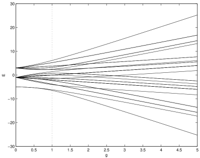
Figure 1: Spectrum of an Ising chain consisting of $5$ particles ($N=5$) as a function of the transverse magnetic field $g$. The dotted line marks the critical point at which the quantum phase transition takes place.

The eigenvalues of Hamiltonian (1) as functions of the transverse field $g$ are visualized in figure 1. It is easily shown that the ground state energy as a function of $g$ is non-analytic at the point $g=1$ in the thermodynamic limit. This non-analytic point is an indication for a quantum phase transition Sachdev (1999) at the quantum critical point $g=1$. This quantum phase transition separates two phases at zero temperature: an ordered phase for $g<1$ and a disordered phase for $g>1$. In the ordered phase, the interaction between the particles aligns the spins parallel or antiparallel to the crystalline axes. In the disordered phase, the external magnetic field induces spin-flips that destroy this order.

The symmetries that Hamiltonian (1) possesses are the $Z_{2}$-symmetry and the translational symmetry. The $Z_{2}$-symmetry corresponds to a reflection of the spin-vectors at the $x$-axes. It is generated by the operator

$$Z_{2}=\prod_{i=0}^{N-1}\sigma_{x}^{(i)}.$$

This operator possesses two different eigenvalues, $1$ and $-1$, such that eigenstates can be classified by two different $Z_{2}$-symmetries. In terms of Fermi operators, states with an even number of fermions possess $Z_{2}$-symmetry $1$ and states with an odd number of fermions possess $Z_{2}$-symmetry $-1$. The translational symmetry is generated by the translation-operator which has the property to right-shift all product states:

$$T|\,z_{1}\,\rangle\cdots|\,z_{N}\,\rangle=|\,z_{N}\,\rangle|\,z_{0}\,\rangle\cdots|\,z_{N-1}\,\rangle$$

This operator possesses $N$ different eigenvalues $e^{-i2\pi n/N}$ ($n=0,\ldots,N-1$), such that the eigenstates can be classified by $N$ different translational symmetries.

II.2 Heisenberg Model

The anisotropic Heisenberg chain Sutherland (1970); Baxter (1972); Kurmann and Thomas (1982) is characterized by anisotropic internal interactions. The Hamiltonian that defines this model reads

$$H=-J\sum_{i=0}^{N-1}\big{\{}\Delta_{x}\sigma_{x}^{(i)}\sigma_{x}^{(i+1)} + \Delta_{y}\sigma_{y}^{(i)}\sigma_{y}^{(i+1)}+$$ (2)

$$+\Delta_{z}\sigma_{z}^{(i)}\sigma_{z}^{(i+1)} + g\,\sigma_{x}^{(i)}\big{\}}.$$

The chain is assumed to be cyclic. The properties of the interactions between the particles of the chain are described by the anisotropy-parameters $\Delta_{x}$, $\Delta_{y}$ and $\Delta_{z}$ and the strength of the external magnetic field is determined by the parameter $g$.

The anisotropic Heisenberg model possesses the same symmetries as the quantum Ising model: the $Z_{2}$-symmetry and the translational symmetry. Thus, eigenstates can be classified by two different $Z_{2}$-symmetries ($1$ and $-1$) and by $N$ different translational symmetries ($e^{-i2\pi n/N}$ with $n=0,\ldots,N-1$).

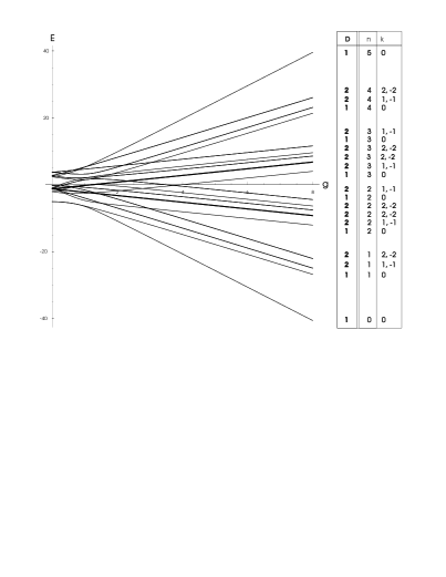
Figure 2: Spectrum of the anisotropic Heisenberg model as a function of the external magnetic field $g$. Assumptions: $N=5$, $\Delta_{x}=0.1$, $\Delta_{y}=0.3$ and $\Delta_{z}=1$; The table on the right hand side gives informations about the degeneracy $D$, the group-index $n$ and the translational-symmetry $k$ of each level.

Another possibility to classify the eigenstates is to classify them according to their behavior in a very strong magnetic field. In figure 2 the energies of the eigenstates are plotted as functions of the field-strength $g$. From this figure it can be gathered that the eigenstates cluster in $N+1$ groups because of the Zeeman-shifts. All states in each group have the property that they tend to the same state in the limit $g\to\infty$. In the $n^{th}$ group, for example, all states tend to a state that has all but $n$ spins aligned in $x$-direction and $n$ spins pointing in $-x$-direction. All eigenstates in the $n^{th}$ group can be classified by a group-index $n$. This group-index is related to the $Z_{2}$-symmetry of the states. It can be shown that states with an even group-index possess the $Z_{2}$-symmetry $1$ and states with an odd group-index possess the $Z_{2}$-symmetry $-1$.

In order to take into account that several eigenstates with group-index $n$ and translational symmetry $k$ may exist, a third index $d$ is required to distinguish eigenstates with equal values for $n$ and $k$. In summary, all eigenstates of $H$ can be identified by the three indices $n$, $k$ and $d$. They will be denoted as

$$|\,\psi_{nkd}\,\rangle,$$

where $n\in\{0,\ldots,N\}$ and $k\in\{0,\ldots,N-1\}$. Evidently, the kets $|\,\psi_{nkd}\,\rangle$ are common eigenstates of $H$, $Z_{2}$ and $T$.

III Quantum simulations of spin systems

Before studying adiabatic processes in spin-systems, a relevant application shall be discussed: the investigation of the ground state of spin-systems with a quantum computer. This investigation could be performed by means of Adiabatic Quantum Computation Farhi et al. (2000); Childs et al. (2001); van Dam et al. (2002).

The scheme of Adiabatic Quantum Computation reads as follows: First, the quantum computer is prepared in the ground state of a simple beginning Hamiltonian, the ground state of which is known. Then, using the Universal Quantum Simulator Lloyd (1996), a time evolution according to a time-dependent Hamiltonian $H(t)$ is simulated which adiabatically interpolates between the simple beginning Hamiltonian and a complicated problem Hamiltonian, the ground state of which shall be investigated. Because of the adiabatic variation, the quantum computer always stays in the ground state of the time-dependent Hamiltonian $H(t)$ and is finally prepared in the ground state of the complicated problem Hamiltonian. Finally, by appropriate measurements, information about the ground state of the problem Hamiltonian is obtained.

Evidently, in the case of spin-systems, the problem Hamiltonian is the Hamiltonian that describes the spin-system of interest. The ground state properties of this Hamiltonian are usually interesting as functions of the strength $g$ of an external magnetic field. Thus, it is obvious to lay out the algorithm such that the field-strength $g$ is adiabatically varied and tunes between the simple beginning Hamiltonian and the problem Hamiltonian. The beginning Hamiltonian can either be the Hamiltonian of the spin-system for $g=0$ or the Hamiltonian of the spin-system for $g\to\infty$. The algorithm then consists either in preparing the quantum computer in the ground state for $g=0$ and adiabatically increasing the field-strength $g$ or in preparing the quantum computer in the ground state for $g\to\infty$ and adiabatically decreasing the field-strength. The ground state for $g\to\infty$ is simple since it has all spins aligned in the direction of the external field. Whether the ground state for $g=0$ can be prepared or not depends on the spin-system under study. In fact, many models exist that are solvable for $g=0$ and, in the case of these models, $g=0$ can be chosen as a starting point.

The duration $T$ of the algorithm is related to the change rate of the parameter $g$. The parameter $g$ must be changed slowly enough, such that the time evolution remains adiabatic. The change rate can be determined mathematically by means of the Adiabatic Theorem Born and Fock (1928); Kato (1950); Friedrichs (1955). This theorem deals with the solution of the Schrödinger equation in the case of a time-dependent and slowly varying Hamiltonian. The statements of the Adiabatic Theorem are the following: In the limit $T\to\infty$, the system always stays in the ground state. Thus, eigenstates of the beginning Hamiltonian are mapped with certainty on eigenstates of the problem Hamiltonian and there is only a change in the phase. In reality, however, the duration $T$ of the time evolution is finite. Thus, the question that has to be answered is how large the duration $T$ must be, such that, with a high probability, the system stays in the ground state. In other words, the probability that eigenstates with higher energy are excited must be negligible.

A rough criterion on the duration $T$ that guarantees that the excitation probability is negligible reads Messiah (1990)

$$T\gg\frac{\mathscr{E}}{\Delta^{2}}.$$ (3)

$\mathscr{E}$ is thereby a quantity that depends on the derivative of the Hamiltonian $H(s)$ with respect to $s$ and $\Delta$ denotes the minimum energy difference between the ground state and the first excited state of $H(s)$. Usually, $\mathscr{E}$ scales polynomially with the number of particles, such that the efficiency mainly depends on the behavior of the minimum energy difference $\Delta$ as a function of the particle number $N$. The energy difference usually reaches its minimum at an avoided level-crossing. At an avoided level-crossing, the ground state and the first excited state approach as the number of particles increases, such that the duration of the algorithm will always increase as the number of particles increases. The efficiency of the algorithm is then determined by the velocity with that the first two states approach. If, on the one hand, the first two states approach exponentially fast with a growing particle number, the algorithm is not efficient. If, on the other hand, the two states approach polynomially fast, the algorithm can be considered to be efficient.

What is seen from this discussion is that knowledge of the spectrum of the Hamiltonian $H(s)$ is required in order to make statements about the duration of the algorithm. However, the spectrum is not known, in general. If the spectrum was known, the ground state of the problem Hamiltonian would be known, as well, and no quantum computer would be required to calculate it. Thus, the only thing that can be done is to test the quantum algorithm on spin-systems that are solvable and see whether it is efficient or not, or to try to find estimations of the spectrum and use them to approximate the duration of the algorithm.

Because of these difficulties in the mathematical determination of the duration of the algorithm, a simple experimental method is desirable that can be used to check whether a chosen change-rate is sufficient or not. An experimental method could look like this: First, the quantum computer is prepared in the ground state of the beginning Hamiltonian, e.g. the Hamiltonian of the spin-system for $g=0$. Then, the field-strength $g$ is increased with a chosen change rate up to a desired value and decreased again with the same change rate. At the end, a measurement in the Eigenbasis of the beginning Hamiltonian is performed (which is known). From this measurement it can be deduced whether the quantum computer is still in the ground state or whether levels with higher energy have been excited. If the quantum computer is still in the ground state, the time evolution was adiabatic and the change rate was low enough. Otherwise, the change rate must be decreased and the experimental check must be performed once again.

IV Adiabatic process in the Ising Model

The adiabatic process under study consists in the slow variation of the strength of the magnetic field that environs the Ising chain, i.e. the slow variation of parameter $g$ in Hamiltonian (1). This variation leads to excitations of states that possess the same symmetry as the initial state of the system (which is assumed to be the ground state).

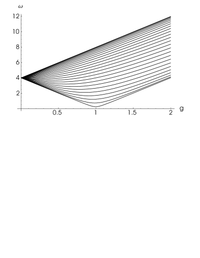
Figure 3: Plot of the excitation energies of the states $|\,n\,\rangle$ as functions of $g$. The assumed number of particles $N$ is $51$.

The symmetries of the problem are, as discussed in section II.1, the $Z_{2}$-symmetry and the translational symmetry. $Z_{2}$-symmetry imposes that only states consisting of an even number of fermions are excited. Translational symmetry makes further restrictions. The states that are excited in first order can be identified by means of the Adiabatic Approximation Messiah (1990). They read

$$|\,n\,\rangle\equiv\eta_{n}^{\dagger}\eta_{-n}^{\dagger}|\,vac\,\rangle,$$

where $n=1,\ldots,\lfloor\frac{N-1}{2}\rfloor$. The energies of these states with respect to the ground state energy are plotted in figure 3 as functions of the field-strength $g$. This figure shows that the energy difference between the lowest excited state and the ground state tends to a minimum at the critical point $g=1$. The minimum energy difference thereby amounts to $\frac{4\pi}{N}$ for $N\gg 1$. This observation already allows to make a qualitative statement about the duration of an adiabatic time evolution in the vicinity of the critical point: Since, according to formula (3), the duration scales with $\frac{1}{\Delta^{2}}$, where $\Delta$ is the minimal energy difference between the lowest exited state and the ground state, the duration can be expected to scale with $N^{2}$, i.e. with the square of the number of particles. This has the consequence that, for example, the investigation of the ground state of the quantum Ising model in the vicinity of the critical point by means of Adiabatic Quantum Computation will be efficient.

These qualitative results can be clarified by calculating the excitation probabilities $p_{0\to n}$ for all states $|\,n\,\rangle$. This can be done analytically by making use of the Adiabatic Approximation Messiah (1990). The details of the analytical calculation can be gathered from appendix B. Another way to calculate the excitation probabilities $p_{0\to n}$ consists in numerically solving the Heisenberg equations for the Fermi-operators $\eta_{k}$. Using this solution, it is simple to calculate expectation values of arbitrary observables after the adiabatic process. If it is assumed that the final state of the system is a superposition of the ground state and the $2$-fermion states $|\,n\,\rangle$ only, the excitation probabilities $p_{0\to n}$ can be calculated as well, since they are expressible in terms of expectation values of the operators $\eta_{n}^{\dagger}\eta_{-n}^{\dagger}\eta_{-n}\eta_{n}$.

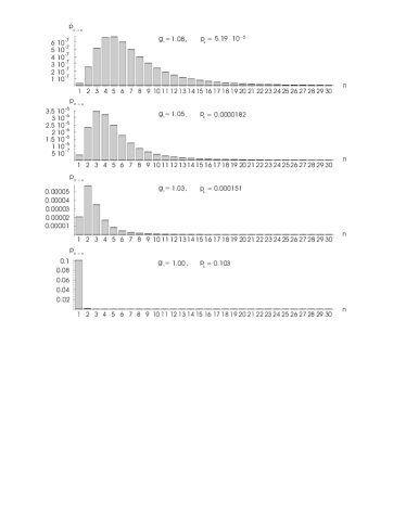
Figure 4: Excitation probability $p_{0\to n}$ of the levels $|\,n\,\rangle$ in the case of $501$ particles ($N=501$). The magnetic field is assumed to be varied from $g_{0}=5$ to $g_{1}$ with change rate $\dot{g}$ equal to $-0.0001$. The indices $n$ are reshuffled such that states with lower index have lower energy.

In figure 4, the excitation probabilities $p_{0\to n}$ are plotted for an Ising chain consisting of $501$ particles. The adiabatic process is assumed to consist in the linear decrease of the magnetic field-strength $g$ with change rate $\dot{g}=-0.0001$ from $g_{0}=5$ to $g_{1}=1.08$, $1.05$, $1.03$ and $1.0$ respectively. It can be observed that, if $g_{1}$ is in the vicinity of the critical point, the lowest state is excited with maximal probability.

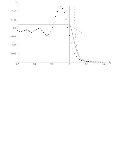
Figure 5: Excitation probability $p_{E}$ as a function of the final field strength $g_{1}$. Assumptions: $51$ particles ($N=51$); linear variation of $g$ from $g_{0}=5$ to $g_{1}$ with change rate $\dot{g}=-0.01$. Solid line: Sum of all terms $p_{0\to n}$; Dotted line: Numerical results (see text); Dashed lines: Analytical estimations (formulas (4) and (5)).

The overall excitation probability $p_{E}$ is obtained by summing the excitation probabilities $p_{0\to n}$ of the respective states. Analytical estimations for the overall excitation probability are obtained in three different regimes:
(1) $g_{0}\gg 1$, $g_{1}>1$ and $N(g_{1}-1)\gg 1$
(2) $g_{0}\gg 1$, $g_{1}>1$ and $N(g_{1}-1)\ll 1$
(3) $g_{0}\gg 1$ and $g_{1}\leq 1$

• In regime (1), the analytical expression for $p_{E}$ reads

  $$p_{E}\lesssim\frac{\hbar^{2}}{2^{8}J^{2}}\frac{(g_{0}-g_{1})^{2}}{T^{2}}\frac{1}{(g_{1}^{2}-1)^{3}}N,$$ (4)

  such that the duration $T$ of the adiabatic process will scale with the square root of the number of particles $N$.

• In regime (2), the overall excitation probability $p_{E}$ can be written as

  $$p_{E}\lesssim\frac{\hbar^{2}}{2^{6}\pi^{4}J^{2}}\frac{(g_{0}-g_{1})^{2}}{T^{2}}(4-3g_{1})N^{4}.$$ (5)

  Thus, the duration $T$ of the adiabatic process will show the previously mentioned $N^{2}$-scaling.

• In regime (3), the overall excitation probability $p_{E}$ is constant as a function of $g_{1}$ (for a fixed change-rate $\dot{g}\equiv(g_{0}-g_{1})/T$), namely,

  $$p_{E}\lesssim\frac{\hbar^{2}}{2^{6}\pi^{4}J^{2}}\frac{(g_{0}-g_{1})^{2}}{T^{2}}N^{4}$$ (6)

  and the duration $T$ of the adiabatic process will show a quadratic scaling with the number of particles $N$, just like in regime (2).

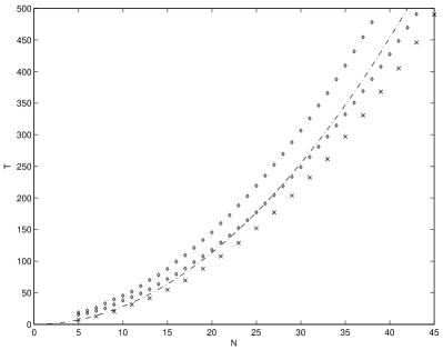
Figure 6: Duration $T$ of the adiabatic process as a function of the particle-number $N$. Assumptions: $g$ is linearly decreased from $g_{0}=5$ to $g_{1}=0$; the change-range $\dot{g}$ is adjusted such that the excitation probability $p_{E}$ always amounts to $0.05$; Crosses: numerical results (see text); Dash-dotted line: analytical result (6), i.e. $T\approx 0.2832N^{2}$. Diamonds: results presented in Dorner et al. (2003) for the free-end chain.

In figure 5, the overall excitation probability $p_{E}$ after the decrease of $g$ from $g_{0}=2$ down to $g_{1}$ is shown as a function of the final field-strength $g_{1}$. The change rate $\dot{g}$ is assumed to be fixed at $-0.01$ and the number of particles is taken to be $51$. The solid line represents the sum of the terms $p_{0\to n}$ that were calculated by means the Adiabatic Approximation. The dashed lines represent the analytical estimations (4) and (5). The dots represent numerical results obtained by solving the Heisenberg equations for the Fermi operators. What can be observed is that the excitation probability increases fundamentally as the critical point $g=1$ is crossed. This behavior is due to the fundamental approach of the ground state and the lowest excited state at the critical point.

The duration $T$ as a function of the number of particles $N$ of an adiabatic process consisting in the linear decrease of the field-strength $g$ from $g_{0}=5$ to $g_{1}=0$ can be gathered from figure 6. The change-rate $\dot{g}$ is thereby adjusted such that the overall excitation probability $p_{E}$ is always equal to $0.05$. The analytic result (6) is represented by the dash-dotted line and the results obtained from numerically solving the Heisenberg equations for the $\eta_{k}$’s are represented by crosses. In both cases, a quadratic scaling of the duration $T$ with the number of particles $N$ can be observed.

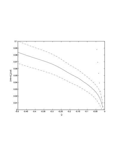
Figure 7: Expectation value of $H$ relative to the width of the spectrum, i.e. $(\langle H\rangle-E_{0})/\Delta E$, as a function of the change-rate $\dot{g}$. Assumptions: $N=51$, $g_{0}=5$ and $g_{1}=0$; solid line: numerical results (see text); dash-dotted line: indicates variance of $H$; dots: results obtained using the Adiabatic Approximation.

Up to now it has been assumed that the field-strength is changed sufficiently slowly, such that the Adiabatic Approximation Messiah (1990) is valid. Outside the adiabatic regime, states with a fermion-number $4,6,8,\ldots$ are excited, additionally to the $2$-fermion states $|\,n\,\rangle$. These states contribute to the overall excitation probability and must be taken into account. However, even outside the adiabatic regime, the mean energy of the system still remains very low. This can be gathered from figure 7. In this figure, the mean energy after the decrease of the field-strength $g$ from $g_{0}=5$ down to $g_{1}=0$ is plotted as a function of the change-rate $\dot{g}$ for a $51$-particle chain. The results about the mean energy were obtained by numerically solving the Heisenberg equations for the $\eta_{k}$’s. As a consequence, processes marginally outside the adiabatic regime prepare the system in a state with very low temperature the properties of which are still interesting to be investigated with a quantum computer.

V Adiabatic process in the Heisenberg Model

The adiabatic process in the anisotropic Heisenberg model is treated similarly as in the previous section: Symmetries are used to determine the states that are excited during the adiabatic process. Since the adiabatic process starts from the ground state, the excited states can be identified as the states that possess the same symmetries as the ground state. Thus, using the notation of section II.2, the excited states are the states with an even group-index $n$ and translational symmetry $k=0$. In practice, only states from the $2^{nd}$ group are excited in first order, namely,

$$|\,\psi_{20d}\,\rangle$$

with $d$ ranging from $1$ to $\frac{N-1}{2}$ ($N$ is assumed to be odd).

Using the previous considerations, it is straightforward to study the efficiency of the algorithm in the case of the anisotropic Heisenberg model. What is required to be done is to find perturbative expansions of the ground state and the possible excited states and to use the Adiabatic Approximation Messiah (1990) to calculate the excitation probabilities. Of course, in order to be allowed to truncate the perturbative expansions after a few lower-order terms, it must be demand that the Hamiltonian consists of parts that are of a different order of magnitude. Because of this, it is assumed that the strength $g$ of the external magnetic field is always much larger than the strength of the internal interactions. The adiabatic process therefore consists in adiabatically decreasing the field strength $g$ from $g_{0}\to\infty$ down to a certain value $g_{1}$, which is still much larger than the strength of the internal interactions ($g_{1}\gg\Delta_{\xi}$).

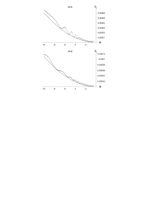
Figure 8: Excitation probability $p_{E}$ as a function of the change rate $\alpha=(g_{1}-g_{0})/T$ in the case of $5$- and $9$-particle chains. Assumptions: $\Delta_{x}=0.1$, $\Delta_{y}=0.3$, $\Delta_{z}=1$; variation of $g$ from $g_{0}=10$ to $g_{1}=5$; Dotted line: Excitation probability obtained from a numerical simulation. Solid line: Approximation (7) of the excitation probability in the limit $N\gg 1$.

The results that are obtained in this way are very similar to results obtained for the quantum Ising model. Details about the calculations can be gathered from appendix C. The analytical expression that is obtained for the overall excitation probability $p_{E}$ reads

$$p_{E}\lesssim\frac{\hbar^{2}}{2^{8}J^{2}}\left(\Delta_{z}-\Delta_{y}\right)^{2}\frac{(g_{0}-g_{1})^{2}}{T^{2}}\frac{1}{g_{1}^{6}}N,$$ (7)

such that the duration $T$ of the adiabatic process will scale with the square root of the number of particles $N$. As a consequence, it will be possible to investigate the ground state of the anisotropic Heisenberg model efficiently by means of Adiabatic Quantum Computation in the regime where the external magnetic field is much stronger than the internal interactions.

The analytical expression (7) can be compared to the exact result (4) presented in section IV for the quantum Ising model. As it is easily verified, the exact result is equal to expression (7) in the limit $g_{1}\gg 1$ if the parameters $\Delta_{x}$, $\Delta_{y}$ and $\Delta_{z}$ are specified to $\Delta_{x}=0$, $\Delta_{y}=0$ and $\Delta_{z}=1$.

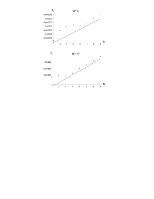
Figure 9: Excitation probability $p_{E}$ as a function of the number of particles $N$ in the case of change rates $\alpha=-6$ and $\alpha=-10$. Assumptions: $\Delta_{x}=0.1$, $\Delta_{y}=0.3$, $\Delta_{z}=1$; variation of $g$ from $g_{0}=10$ to $g_{1}=5$; Dotted line: Excitation probability obtain from a numerical simulation. Solid line: Approximation (7) of the excitation probability in the limit $N\gg 1$.

Expression (7) can also be compared to results obtained from numerical simulations. This is shown in figures 8 and 9. In these figures, the excitation probability is plotted as a function of the change rate $\dot{g}$ and as a function of the particle-number $N$ respectively. The dots represent the results from numerical simulations and the solid lines represent evaluations of the analytical formula (7). It is seen that the numerical results for the excitation probability scale linearly with the number of particles $N$ and they scale quadratically with the change rate $\dot{g}$, as it is stated by formula (7).

VI Stability

In this section, the implication of perturbations that accompany the adiabatic process shall be discussed. These perturbations occur, for example, if the adiabatic process is simulated on a quantum computer and quantum gates are not implemented perfectly. The problem that arises is that perturbations usually break the symmetry of the original Hamiltonian, such that, in principle, excitations of levels with very low energy may occur. The question that has to be answered in this connection is whether these excitations spoil previous results or not.

In the case of the quantum Ising model, the answer to this question can be found using time-dependent perturbation theory with respect to the perturbation. The perturbation is thereby assumed to be given by

$$V=J\varepsilon\,\sigma_{z}^{(0)}.$$

If the adiabatic process consists in the slow decrease of the field-strength $g$ from $g_{0}\gg 1$ to $g_{1}<1$, then, after crossing the critical point, this perturbation leads to a strong excitation of the (asymptotically degenerate) first excited state and a very small excitation of states with higher energy. Nevertheless, the mean energy of the system after excitation is still very low compared to the width of the spectrum $\Delta E$, namely,

$$\frac{\langle H\rangle-E_{0}}{\Delta E}=const\,\varepsilon^{2}.$$

This term doesn’t depend on the number of particles $N$ and is negligible for $\varepsilon\ll 1$ even for large $N$. Thus, it can be concluded that, even though an adiabatic process accompanied by small perturbations will not leave the system in the ground state, it will prepare the system in a state with very low temperature. Such a low-temperature state also shows properties which are interesting to be investigated with a quantum computer.

In the case of the anisotropic Heisenberg model, the perturbation term is assumed to be more general, namely,

$$V=J\sum_{j=0}^{N-1}\varepsilon_{j}\,\vec{n}^{(j)}\cdot\vec{\sigma}^{(j)},$$

with $\varepsilon_{j}\in\mathbb{R}$ and $|\vec{n}^{(j)}|=1$. The adiabatic process, however, is assumed to be restricted to the regime where the external magnetic field is much stronger than the internal interactions. The probability that the perturbation $V$ causes an excitation during this process is then estimated as

$$p_{V}\lesssim\left(\frac{\varepsilon}{2g_{0}}\right)^{2}N$$

where $\varepsilon$ is defined as

$$\varepsilon:=\sqrt{\frac{1}{N}\sum_{j=0}^{N-1}\varepsilon_{j}^{2}\left|n_{x}^{(j)}+in_{y}^{(j)}\right|^{2}}.$$

From this formula it can be read off that the excitation-probability $p_{V}$ scales polynomially with the error-parameter $\varepsilon$ and the number of particles $N$. Thus, small perturbations during the adiabatic process will not have severe implications.

VII Conclusions

Summing up, adiabatic processes have been investigated in the light of the simple, exactly solvable quantum Ising model and the more complicated anisotropic Heisenberg model. The adiabatic processes were assumed to consist in the slow variation of the strength of the magnetic field that environs the spin-chains.

In the case of the quantum Ising model, the investigation could be performed in detail and analytic results were obtained even for processes that cross the quantum critical point. In the case of the anisotropic Heisenberg model, adiabatic processes were studied in regimes amenable to perturbative treatment. In both cases, the duration of the adiabatic processes turned out to scale polynomially with the number of particles the spin-systems consist of.

The results that were obtained are relevant for the treatment of bosons in optical lattices and for Adiabatic Quantum Computation. In Adiabatic Quantum Computation, light is shed on the efficiency of adiabatic quantum algorithms that investigate the ground state of spin-systems. In the treatment of optical lattices, insight is gained into the dynamics of quantum phase transitions.

As an outlook on future work, adiabatic processes in more complicated, yet unsolved models, such as higher-dimensional spin-systems or spin-glasses, could be studied, such that information is gained about quantum phase transitions in these models and about the efficiency of adiabatic quantum algorithms investigating the ground state of these models.

Appendix A Diagonalization of the Quantum Ising-Hamiltonian

Jordan-Wigner transformation Lieb et al. (1961) of Hamiltonian (1) leads to a Hamiltonian consisting of two parts: a part that is quadratic in terms of Fermi operators and a non-quadratic part:

$$H/J = -\sum_{i=0}^{N-1}\Big{\{}\big{(}c_{i}^{\dagger}c_{i+1}+c_{i}^{\dagger}c_{i+1}^{\dagger}+\textrm{h.c.}\big{)}-2gc_{i}^{\dagger}c_{i}\Big{\}}+$$

$$+\big{(}c_{N-1}^{\dagger}c_{0}+c_{N-1}^{\dagger}c_{0}^{\dagger}+\textrm{h.c.}\big{)}\big{(}e^{i\pi\hat{N}}+1\big{)}-gN$$

The Fermi-operators $c_{j}$ are chosen to be periodic, i.e. $c_{j+N}\equiv c_{j}$. The symbol $\hat{N}$ denotes the fermion number operator which is defined as $\hat{N}=\sum_{i=0}^{N-1}c_{i}^{\dagger}c_{i}$. Even though the non-quadratic term can be neglected for many calculations because it only makes changes of order $\frac{1}{N}$ to eigenvalues and eigenstates Sachdev (1999); Pfeuty (1970), it is fundamental for the investigation of the quantum dynamics in the vicinity of the critical point $g=1$. This is because the ground state and the lowest excited state approach according to $\frac{4\pi}{N}$ in the vicinity of the critical point as the number of particles $N$ increases (see figure 3). Thus, corrections of order $\frac{1}{N}$ cannot be neglected even if $N$ is large.

Since the non-quadratic term $e^{i\pi\hat{N}}$ is invariant under linear transformations between Fermi-operators Lieb et al. (1961), diagonalization can be performed separately in two subspaces consisting of an even and an odd number of fermions. In the odd-fermion-number subspace, $e^{i\pi\hat{N}}$ simplifies to $-1$ and the remaining quadratic Hamiltonian can be diagonalized by linearly transforming the set of Fermi-operators $c_{j}$ into a set of Fermi-operators $\bar{\eta}_{j}$ in terms of which Hamiltonian (1) is diagonal:

$$H/J=gN+\sum_{k=0}^{N-1}\bar{\Lambda}_{k}\left(\bar{\eta}_{k}^{\dagger}\bar{\eta}_{k}-\frac{1}{2}\right)$$ (8)

The energy $\bar{\Lambda}_{k}$ of a single $\bar{\eta}_{k}$-fermions is calculated as

$$\bar{\Lambda}_{k}=2\left\{\begin{array}[]{lcl}g-1,&&k=0\\ \sqrt{1+g^{2}-2g\cos\frac{2\pi k}{N}},&&k\neq 0\\ \end{array}\right\}.$$ (9)

In the even-fermion-number subspace $e^{i\pi\hat{N}}$ equals $1$ and diagonalization yields

$$H/J=gN+\sum_{k=0}^{N-1}\Lambda_{k}\left(\eta_{k}^{\dagger}\eta_{k}-\frac{1}{2}\right)$$ (10)

with

$$\Lambda_{k}=2\sqrt{1+g^{2}+2g\cos\frac{2\pi k}{N}}$$ (11)

being the energy of one single $\eta_{k}$-fermion.

The ground state of Hamiltonian (1) is the vacuum-state $|\,vac\,\rangle$ in the even-fermion-number subspace. The first excited state is the $1$-fermion state $\bar{\eta}_{0}^{\dagger}|\,vac\,\rangle$ lying in the odd-particle subspace. The energy difference between these two states amounts to

$$\Delta E(g)=(g-1)+\sqrt{(g-1)^{2}+g\left(\frac{\pi}{N}\right)^{2}}$$

for $N\gg 1$. This energy difference tends to zero for $g\leq 1$ in the thermodynamic limit, which is known as asymptotic degeneracy Pfeuty (1970).

Appendix B Calculating the Dynamics of the Ising Model

Adiabatic processes are conveniently treated by means of the Adiabatic Approximation Messiah (1990). The Adiabatic Approximation allows to calculate in first order the probability that, during an adiabatic passage, states above the ground state are excited. If it is assumed that the adiabatic process consists in the variation of the parameter $s$ from $0$ to $1$ during time $T$, the first order excitation probabilities read

$$p_{0\to j}(T)\lesssim\frac{1}{T^{2}}\max_{0\leq s\leq 1}\left|\frac{A_{j0}(s)}{\omega_{j0}(s)}\right|^{2}$$ (12)

with

$$A_{j0}(s) = -\frac{\langle\,\psi_{j}(s)\,|\frac{dH}{ds}|\,\psi_{0}(s)\,\rangle}{\hbar\omega_{j0}(s)}$$

$$\hbar\omega_{j0}(s) = E_{j}(s)-E_{0}(s).$$

$|\,\psi_{j}(s)\,\rangle$ and $E_{j}(s)$ thereby denote the $j^{th}$ Eigenstate of $H(s)$ and its corresponding Eigenvalue. A definite statement about the duration of the adiabatic process is finally obtained by demanding that the overall excitation probability must be negligible, i.e. $p_{E}\equiv\sum_{j\neq 0}p_{0\to j}(T)\ll 1$.

In the adiabatic process investigated here, the field-strength $g$ is varied linearly from $g_{0}$ to $g_{1}$ during time $T$. In terms of the previously introduced formalism, $g$ is dependent on the parameter $s$ according to the formula

$$g(s)=g_{0}+s(g_{1}-g_{0})$$

and $s$ is varied from $0$ to $1$ as time evolves from $0$ to $T$.

Since the adiabatic passage starts from the ground state (lying in the even-fermion-number subspace) and the evenness and oddness of states is conserved during time evolution because of the $Z_{2}$-symmetry, calculations can be restricted to the even-fermion-number subspace. In this subspace, the dynamics are governed by Hamiltonian (10).

The excitation probability can now be calculated by means of formula (12). However, the determination of the functions $A_{j0}(s)$ requires the knowledge of the derivative of $H(s)$ with respect to the parameter $s$. This derivative can be calculated easily if it is taken into account that (for an odd number $N$ of spins)

$$\frac{d}{ds}\eta_{k}(s)=-\frac{\theta_{k}^{\prime}(s)}{2}\left(\eta_{-k}(s)-\eta_{-k}^{\dagger}(s)\right),$$

with

$$\theta_{k}^{\prime}(s)=\frac{dg}{ds}\,\frac{\sin\frac{2\pi k}{N}}{1+g(s)^{2}+2g(s)\cos\frac{2\pi k}{N}}.$$

The derivative $H^{\prime}(s)$ couples the vacuum state $|\,vac(s)\,\rangle$ only to the vacuum state itself and to the two-fermion states

$$|\,n(s)\,\rangle:=\eta_{n}^{\dagger}(s)\eta_{-n}^{\dagger}(s)|\,vac(s)\,\rangle,\quad n=1,\ldots,\lfloor\frac{N-1}{2}\rfloor.$$

The only states that are excited (in first order) during the adiabatic passage are therefore the two-fermion states $|\,n(s)\,\rangle$. The matrix element of $H^{\prime}(s)$ that describes the coupling between the states $|\,n(s)\,\rangle$ and $|\,vac(s)\,\rangle$ reads

$$\langle\,n(s)\,|H^{\prime}(s)|\,vac(s)\,\rangle=-J\Lambda_{n}(s)\theta_{n}^{\prime}(s).$$

In addition, the energy difference between $|\,n(s)\,\rangle$ and the ground state amounts to

$$\hbar\omega_{n0}(s)=2J\Lambda_{n}(s).$$

The probability that the two-fermion states $|\,n(s)\,\rangle$ are excited can now be calculated using formula (12):

$$p_{0\to n}\lesssim\frac{\hbar^{2}}{2^{4}J^{2}}\frac{1}{T^{2}}\max_{0\leq s\leq 1}\left|\frac{\theta_{n}^{\prime}(s)}{\Lambda_{n}(s)}\right|^{2}$$

The overall excitation probability $p_{E}$, i.e. the probability that any state above the ground state is excited during the adiabatic process, is equal to the sum over all terms $p_{0\to n}$. This sum can be evaluated for $N\gg 1$ either by replacing the sum by an integral yielding result (4) or by explicitly summing over approximated addends yielding results (5) and (6).

Appendix C Calculating the Dynamics of the Heisenberg Model

As in the previous section, the probability that the system is, at the end of the adiabatic process, in an excited state can be calculation by means of formula (12). The calculation of the quantities $A_{j0}(s)$ and $\hbar\omega_{j0}(s)$, however, requires the knowledge of the eigenstates and eigenvalues of Hamiltonian (2). The series expansions about $g\to\infty$ of the ground state energy $E_{0}(s)$ and the ground state $|\,\psi_{0}(s)\,\rangle$ read

$$\frac{E_{0}(s)}{JN}=-g(s)-\Delta_{x}+\textrm{O}\left[\frac{1}{g}\right]$$

and

$$|\,\psi_{0}(s)\,\rangle\propto|\,\varphi_{0}^{(0)}\,\rangle+\frac{1}{g(s)}|\,\varphi_{0}^{(1)}\,\rangle+\textrm{O}\left[\frac{1}{g}\right]^{2}.$$

The coefficients $|\,\varphi_{0}^{(0)}\,\rangle$ and $|\,\varphi_{0}^{(1)}\,\rangle$ are thereby defined as

$$|\,\varphi_{0}^{(0)}\,\rangle = |\rightarrow\rangle$$

$$|\,\varphi_{0}^{(1)}\,\rangle = \frac{1}{4}\left(\Delta_{z}-\Delta_{y}\right)\sum_{j=0}^{N-1}|\,j,j+1\,\rangle.$$

The symmetries that the ground state possesses are the $Z_{2}$-symmetry $1$ and the translational-symmetry $k=0$. The only states that can be excited during a time evolution according to $H(s)$ are states that possess the same symmetries as the ground state. The lowest states that meet this requirement are the states with group-index $n=2$ and translational-symmetry $k=0$, namely,

$$|\,\psi_{20d}(s)\,\rangle.$$

The energies of these states are $E_{20d}(s)$. In the case of an odd number of particles $N$, the series expansions about $g\to\infty$ of $E_{20d}(s)$ and $|\,\psi_{20d}(s)\,\rangle$ read

$$\frac{E_{20d}(s)}{JN} = -g(s)\left(1-\frac{4}{N}\right)-\Delta_{x}\left(1-\frac{8}{N}\right)+$$

$$+\frac{4}{N}\left|\Delta_{z}+\Delta_{y}\right|\cos\frac{2\pi d}{N+1}+\textrm{O}\left[\frac{1}{g}\right]$$

and

$$|\,\psi_{20d}(s)\,\rangle\propto|\,\varphi_{20d}^{(0)}\,\rangle+\frac{1}{g(s)}|\,\varphi_{20d}^{(1)}\,\rangle+\textrm{O}\left[\frac{1}{g}\right]^{2}.$$

The index $d$ may thereby assume the values $1,\ldots,\frac{N-1}{2}$. The coefficients $|\,\varphi_{20d}^{(0)}\,\rangle$ and the projection of $|\,\varphi_{20d}^{(1)}\,\rangle$ on $|\rightarrow\rangle$ are given by

$$|\,\varphi_{20d}^{(0)}\,\rangle = \frac{2}{\sqrt{N+1}}\,\sum_{j=1}^{\frac{N-1}{2}}\sin\frac{2\pi dj}{N+1}|\,\Upsilon_{20j}\,\rangle$$

$$\langle\rightarrow|\,\varphi_{20d}^{(1)}\,\rangle = -\frac{1}{2}(\Delta_{z}-\Delta_{y})\sqrt{\frac{N}{N+1}}\sin\frac{2\pi d}{N+1}.$$

The kets $|\,\Upsilon_{20j}\,\rangle$ that appear in the upper formula denote the $2$-particle states with translational symmetry $k=0$. They are defined as

$$|\,\Upsilon_{20j}\,\rangle=\frac{1}{\sqrt{N}}\sum_{i=0}^{N-1}|\,i,i+d\,\rangle.$$

In order to calculate the functions $A_{j0}(s)$, the matrix elements of the derivative $H^{\prime}(s)$ between the ground state $|\,\psi_{0}(s)\,\rangle$ and the excited states $|\,\psi_{20d}(s)\,\rangle$ must be determined. It is advantageous to abbreviate these matrix elements by the notation $\mathcal{H}_{d0}(s)$:

$$\mathcal{H}_{d0}(s):=\langle\,\psi_{20d}(s)\,|H^{\prime}(s)|\,\psi_{0}(s)\,\rangle$$

The derivative $H^{\prime}(s)$ is equal to the expression

$$H^{\prime}(s)=-Jg^{\prime}(s)\sum_{i=0}^{N-1}\sigma_{x}^{(i)}.$$

Using this expression and the series expansions of $|\,\psi_{0}(s)\,\rangle$ and $|\,\psi_{20d}(s)\,\rangle$, it is straightforward to determine the matrix elements $\mathcal{H}_{d0}(s)$: The contribution to $\mathcal{H}_{d0}(s)$ to $0^{th}$-order in $\frac{1}{g}$ is zero. This is because the derivative $H^{\prime}(s)$ does not couple the $0^{th}$-order-coefficients $|\,\varphi_{0}^{(0)}\,\rangle$ and $|\,\varphi_{20d}^{(0)}\,\rangle$. To $1^{st}$ order in $\frac{1}{g}$, the terms $\langle\,\varphi_{20d}^{(1)}\,|H^{\prime}(s)|\,\varphi_{0}^{(0)}\,\rangle$ and $\langle\,\varphi_{20d}^{(0)}\,|H^{\prime}(s)|\,\varphi_{0}^{(1)}\,\rangle$ contribute. Higher-order contributions to $\mathcal{H}_{d0}$ will not be taken into account. In summary, the series expansion to lowest order in $\frac{1}{g}$ of the matrix element $\mathcal{H}_{d0}$ reads

$$\mathcal{H}_{d0}(s)=\frac{1}{g(s)} \Big{\{} \langle\,\varphi_{20d}^{(1)}\,|H^{\prime}(s)|\,\varphi_{0}^{(0)}\,\rangle+$$

$$+ \langle\,\varphi_{20d}^{(0)}\,|H^{\prime}(s)|\,\varphi_{0}^{(1)}\,\rangle\,\Big{\}}+\textrm{O}\left[\frac{1}{g}\right]^{2}.$$

A simplification of this expression yields

$$\mathcal{H}_{d0}(s)=-2\left(\Delta_{z}-\Delta_{y}\right)\frac{g^{\prime}(s)}{g(s)}\sqrt{\frac{N}{N+1}}\sin\frac{2\pi d}{N+1}+\textrm{O}\left[\frac{1}{g}\right]^{2}.$$

The probability $p_{0\to d}$ that the states $|\,\psi_{20d}(s)\,\rangle$ are excited can now easily be calculated using formula (12). The overall excitation probability $p_{E}$ is equal to the sum over all terms $p_{0\to d}$. In the limit of a large number of particles ($N\gg 1$), this sum can be approximated by an integral. This approximation leads to a simplified expression for the overall excitation probability $p_{E}$, namely, result (7).

References

- Jaksch et al. (1998) D. Jaksch, C. Bruder, J. I. Cirac, C. W. Gardiner, and P. Zoller, Phys. Rev. Lett 81, 3108 (1998).
- Greiner et al. (2002) M. Greiner, O. Mandel, T. Esslinger, T. W. Hänsch, and I. Bloch, Nature 415, 39 (2002).
- Jané et al. (2002) E. Jané, G. Vidal, W. Dür, P. Zoller, and J. I. Cirac, Quant. Inf. Comp. 3, 15 (2002), eprint quant-ph/0207011.
- Duan et al. (2002) L. M. Duan, E. Demler, and M. D. Lukin (2002), eprint cond-mat/0210564.
- García-Ripoll and Cirac (2003) J. J. García-Ripoll and J. I. Cirac, Phys. Rev. Lett. 90, 127902 (2003).
- Dorner et al. (2003) U. Dorner, P. Fedichev, D. Jaksch, M. Lewenstein, and P. Zoller (2003), eprint quant-ph/0212039.
- Sachdev (1999) S. Sachdev, Quantum Phase Transitions (Cambridge University Press, 1999).
- Farhi et al. (2000) E. Farhi, J. Goldstone, S. Gutmann, and M. Sipser (2000), eprint quant-ph/0001106.
- Childs et al. (2001) A. M. Childs, E. Farhi, and J. Preskill, Phys. Rev. A 65, 012322 (2001).
- van Dam et al. (2002) W. van Dam, M. Mosca, and U. Vazirani (2002), eprint quant-ph/0206003.
- Feynman (1982) R. P. Feynman, Int. J. Theor. Phys. 21, 467 (1982).
- Lloyd (1996) S. Lloyd, Science 273, 1073 (1996).
- Abrams and Lloyd (1997) D. S. Abrams and S. Lloyd, Phys. Rev. Lett. 79, 2586 (1997).
- Wu et al. (2002) L. A. Wu, M. S. Byrd, and D. A. Lidar, Phys. Rev. Lett. 89, 057904 (2002).
- Pfeuty (1970) P. Pfeuty, Annals of Physics 57, 79 (1970).
- Lieb et al. (1961) E. Lieb, T. Schultz, and D. Mattis, Annals of Physics 16, 407 (1961).
- Sutherland (1970) B. Sutherland, J. Math. Phys. 11, 3183 (1970).
- Baxter (1972) R. J. Baxter, Annals of Physics 70, 323 (1972).
- Kurmann and Thomas (1982) J. Kurmann and H. Thomas, Physica 112A, 235 (1982).
- Born and Fock (1928) M. Born and V. Fock, Z. Phys. 51, 165 (1928).
- Kato (1950) T. Kato, J. Phys. Soc. Jap. 5, 435 (1950).
- Friedrichs (1955) K. Friedrichs, Report IMM NYU-218 (1955).
- Messiah (1990) A. Messiah, Quantenmechanik, Band 2 (Walter de Gruyter, 1990).