]http://www.quantware.ups-tlse.fr

Treatment of sound on quantum computers

Abstract

We study numerically how a sound signal stored in a quantum computer can be recognized and restored with a minimal number of measurements in presence of random quantum gate errors. A method developed uses elements of MP3 sound compression and allows to recover human speech and sound of complex quantum wavefunctions.

In the last decade the rapid technological progress made possible the treatment of large amounts of information and their transmission over large distances. In spite of this the transmission of digital audio signals required the development of specific compression methods in order to achieve real time audio communication. A well known example of audio compression is the Mpeg Audio Layer 3 (MP3) which allows to reduce the signal size by an order of magnitude without noticeable distortion mp3 . It essentially uses the Fast Fourier Transform (FFT) in order to have rapid access to the signal spectrum, whose analysis allows to reach significant compression rates. Such methods find every day applications in the Internet telephone communication and teleconferences.

Recent developments in quantum information make possible a new type of computation and communication using the quantum nature of the signal (see e.g. chuang ; qcom ). In quantum computation theory it was shown that certain quantum algorithms can be exponentially more efficient than any known classical counterpart. For instance the Shor algorithm enables to factorize large integers in a time polynomial in the number of bits whereas all known classical algorithms are exponential shor . This algorithm relies on the Quantum Fourier Transform (QFT) which is exponentially faster than FFT chuang ; shor . Simple quantum algorithms have been realized experimentally with few qubit quantum computers based on Nuclear Magnetic Resonance (NMR) and ion traps chuang1 ; cory ; blatt . Quantum communications also attracted a great deal of attention since they allow to realize secret data transmission. Currently, such a transmission has been achieved over distances of up to a few tens kilometers qcom .

These prospects rise timely the question of treatment of audio signals on quantum computers. Classical audio analysis methods cannot be directly applied to quantum signals and it is important to adapt them to the new environment of quantum computation. Furthermore while digital signal treatment is faultless, quantum computation contains phase and amplitude errors which can affect the quality of sounds encoded on a quantum computer. In addition the extraction of quantum information relies on quantum measurements which bring new elements that must be taken into account in the treatment of quantum audio signals. Different type of sound signals are possible like human speech, music or pure quantum objects like the Wigner function wigner which can be efficiently prepared on quantum computers laflamme ; levi .

For the standard audio sampling rate of $44kHz$ a quantum computer with $20$ qubits (two-level quantum systems, see chuang ) can store a mono audio signal of $23$ seconds. A quantum computer with $50$ qubits may store an amount of information exceeding all modern supercomputer capacities (1000 years of sound). Thus the development of readout methods, which in presence of imperfections can recognize and restore the sound signal via a minimal number of quantum measurements, becomes of primary importance.

To study this problem we choose the following soundtrack pronounced by HAL in the Kubrick movie “2001: a space odyssey”: “Good afternoon, gentlemen. I am a HAL 9000 computer. I became operational at the H.A.L. lab in Urbana, Illinois on the 12th of January” hal . The duration of this recording is 26 seconds and at a sampling rate $f=8kHz$ it can be encoded in the wavefunction of a quantum computer with $n_{q}=18$ qubits (the HAL speech is thus zero padded to last 32 seconds). This rate gives good sound quality and is more appropriate for our numerical studies. Digital audio signals can be represented by a sequence of samples with values $s_{n}$ in the interval $(-1,1)$ so that the $n$-th sample gives the sound at time $t=n/f$. This signal can be encoded on a quantum computer by the following wavefunction $\psi=A\sum_{n}s_{n}|n>$, where $A$ is normalization constant. The state $|n>$ represents the multiqubit eigenstate $|a_{1}...a_{i}...a_{n_{q}}>$ where $a_{i}$ is 0 or 1 corresponding to the lower or upper qubit state, the sequence of $a_{i}$ gives the binary representation of $n$.

Using numerical simulations we test various approaches to the readout problem of the above signal encoded in the wavefunction of a quantum computer. Direct measurements of the wavefunction do not allow to keep track of the sign of $s_{n}$ and many measurements are required to determine the amplitude $|s_{n}|$ with good accuracy. Another strategy is to use the analogy with the MP3 coding. With this aim we divide the sound into consecutive frames of fixed size $\Delta n=2^{n_{f}}$ where $n_{f}$ can be viewed as the number of qubits required to store one frame. We choose these qubits to be the $n_{f}$ least significant qubits in the binary representation of $n=(a_{1}...a_{n_{q}-n_{f}+1}...a_{n_{q}})$. Then we perform QFT on these $n_{f}$ qubits that corresponds to applying FFT to all the $2^{n_{q}-n_{f}}$ frames of the signal in parallel. This requires $n_{f}(n_{f}+1)/2$ quantum gates contrary to $O(n_{f}2^{n_{f}})$ classical operations for FFT. After this transformation the wavefunction represents the instantaneous spectrum of the sound signal evolving in time from one frame to another. This way the most significant $n_{q}-n_{f}$ qubits store the frame number $k$ while the least significant $n_{f}$ qubits give the frequency harmonic number $j$. Hence, after QFT the wave function has the form $\psi=\sum_{k,j}S_{k,j}|k,j>$ where $S_{k,j}$ is the complex amplitude of the $j$-th harmonic in the $k$-th frame. The measurements in this representation gives the amplitudes $|S_{k,j}|$ while phase information is lost. However for sound the main information is stored in the spectrum amplitudes and the ear can recover the original speech even if the phases are all set to zero. Thus the recovered signal is obtained by the inverse classical FFT and is given by $s^{\prime}_{n}=\sum_{j}|S_{k,j}|e^{2\pi ijm/\Delta n}$ with $n=k\;\Delta n+m$ (to listen sound we use $Re(s^{\prime}_{n})$). For time domain measurements of $s_{n}$ the recovered signal is $\tilde{s}_{n}=|s_{n}|$. These expressions for $s^{\prime}_{n}$ and $\tilde{s}_{n}$ hold for an infinite number of measurements. In reality it is important to approximate them accurately with a minimal number of measurements.

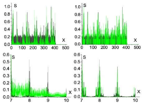
Figure 1: (color online) Sound signal spectrum as a function of frame number $x=n/\Delta n$. On all panels the black curves show the spectrum of the original signal $s_{n}$. On the left top panel the green/gray curve represents the spectrum of $\tilde{s}_{n}$ obtained with $M=5$ measurements per frame in time domain. On the right top panel it shows the spectrum of $s^{\prime}_{n}$ for the same number of measurements $M$ performed after QFT. Bottom panels show these spectra on a smaller scale.

For our soundtrack we found that the optimal frame size is $\Delta n=2^{9}(n_{f}=9)$ and we perform $M$ measurements per frame. In Fig. 1 we compare the spectrum of $s^{\prime}_{n}$ and $\tilde{s}_{n}$ with the original signal spectrum. Here only $M=5$ measurements per frame are performed and the results clearly show that the quality of the restored sound is significantly higher for the spectrum domain measurements. Examples of restored and original sounds are available at qaudiosite . The HAL speech is recognizable from $M=5$ for spectrum domain measurements while it is distorted beyond recognition for direct time domain measurements even for $M=100$.

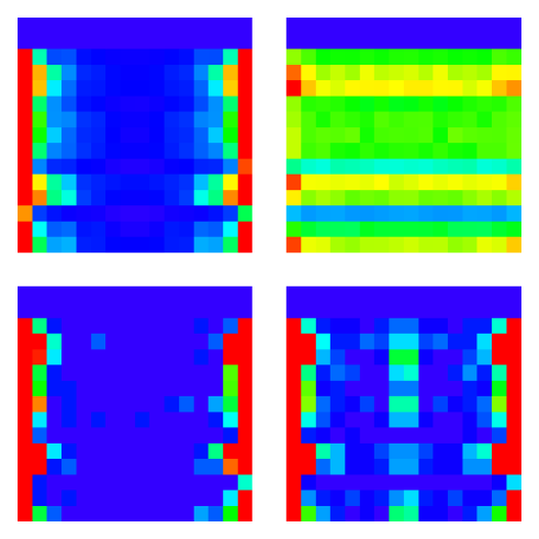
Figure 2: (color) Coarse grained diagram for the signal of Fig. 1 obtained by measurements of qubits 1 to 4 and 10 to 13 (see text). Top left: original signal; bottom left: distribution obtained after QFT with the same number of measurements as in Fig. 1; bottom right: same as bottom left with the noise in the quantum gates ($\epsilon=0.05$); top right: diagram obtained from measurements in time domain (with the same number of measurements as in bottom right). The color represents amplitude of the spectrum: blue for zero and red for maximal values. The horizontal/vertical axis corresponds to coarse grained frequency/time.

Fig. 1 shows the global structure of the signal spectrum. To make comparison more quantitative and visual we show coarse grained color diagrams of the spectrum. The coarse graining is obtained by measuring only certain qubits corresponding for example to $a_{1}a_{2}a_{3}a_{4}$ and $a_{10}a_{11}a_{12}a_{13}$. For $s^{\prime}_{n}$ this gives a coarse grained spectrum $|S_{k,j}|$ in $2^{4}\times 2^{4}$ cells shown in Fig. 2. The same total number of measurements as in Fig. 1 allows to reproduce the original coarse grained diagram with good accuracy. Even if QFT is performed with noisy gates (the angle in the unitary rotations fluctuates with an amplitude $\epsilon\pi=0.05\pi$) the spectrum diagram remains stable and is reproduced with good accuracy (see Fig. 2). At the same time the coarse graining in the time domain for the signal $\tilde{s}_{n}$ shown in Fig. 1 gives the diagram which is very different from the original.

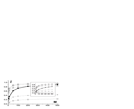
Figure 3: Fidelity $\tilde{f}$ for sound signals $s^{\prime}_{n}$ (open circles) and $\tilde{s}_{n}$ (full circles) as a function of number of measurements $M$. For $s^{\prime}_{n}$ fidelity is shown for various amplitudes of noise in the QFT gates with $\epsilon=0$ (o), 0.05 (diamonds), 0.1 (triangles), 0.3 (+), 1 (squares). Inset shows data at small $M$ scale.

The global quality of the recovered signal $\tilde{s}_{n}$ (or $s^{\prime}_{n}$) obtained via a finite number of measurements is convenient to characterize by the fidelity defined as $\tilde{f}=|\sum_{n}{\tilde{s}^{(^{\prime})*}_{n}\tilde{s}^{(^{\prime})}_{n}(M,\epsilon)}|/R$ with $R=(\sum_{n}{|\tilde{s}^{(^{\prime})}_{n}|^{2}}\sum_{n}{|\tilde{s}^{(^{\prime})}_{n}(M,\epsilon)|^{2}})^{1/2}$. Here, $\tilde{s}^{(^{\prime})}_{n}(M,\epsilon)$ is the signal obtained in a way described above with $M$ measurements per frame in time domain $(\tilde{s}_{n}(M))$ or in frequency domain after QFT with noisy gates $(s^{\prime}_{n}(M,\epsilon))$. The dependence of $\tilde{f}$ on $M$ is shown in Fig. 3. For large $M$ it approaches to unity for both signals $\tilde{s}_{n}$ and $s^{\prime}_{n}$ at $\epsilon=0$. However, for a small number of measurements $(5\leq M\leq 50)$ the fidelity is significantly higher for measurements performed in the frequency domain after QFT (Fig. 3 inset). The presence of noise in the quantum gates used in QFT for $s^{\prime}_{n}$ reduces the value of $\tilde{f}$ but for $5\leq M\leq 50$ and $\epsilon\leq 0.1$ this reduction is not significant. The drop of $\tilde{f}$ becomes considerable only at relatively large amplitudes with $\epsilon>0.2$ as it is shown in Fig. 4. The residual level of $\tilde{f}$ at maximal $\epsilon\approx 1$ is in agreement with the statistical estimate according to which $\tilde{f}(\epsilon=1)\approx\sqrt{n_{i}/2^{n_{f}}}\approx 0.2$, where $n_{i}$ is the number of frequencies per frame for the original signal ($n_{i}\approx 20$ according to Fig. 2). At small $\epsilon$ the drop of $\tilde{f}$ is quadratic in $\epsilon$ ($1-\tilde{f}\sim\epsilon^{2}n_{f}^{2}$) since each gate transfers about of $\epsilon^{2}$ amount of probability from ideal computational state to all other states levi . The obtained results show that the MP3-like strategy adapted to the quantum signals allows to recover human speech with a significantly smaller number of measurements with a reduction factor of 10-20.

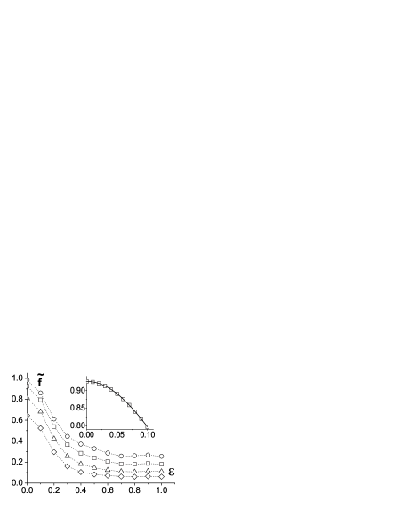
Figure 4: Dependence of fidelity $\tilde{f}$ for the sound signal $s^{\prime}_{n}$ on the noise amplitude $\epsilon$ for the number of measurements $M=1000$ (o), 100 (squares), 20 (triangles), 5 (diamonds). Inset shows a data fit $1-\tilde{f}=0.36\epsilon^{2}n_{f}^{2}$ (full curve) at small $\epsilon$, $M=100$.

Above we assumed that the sound signal is already encoded in the wavefunction. For certain quantum objects such an encoding can be done efficiently. As an example we consider the wavefunction evolution described by the quantum sawtooth map

$$\overline{\psi}=\hat{U}\psi=e^{-iT\hat{l}^{2}/2}e^{ik\hat{\theta}^{2}/2}\psi,$$ (1)

where $\hat{l}=-i\partial/\partial\theta$, $\hbar=1$, $k,T$ are dimensionless map parameter and $\overline{\psi}$ is the value of $\psi$ after one map iteration (we set $\hbar=1$). In the semiclassical limit $k\gg 1$, $T\ll 1$ the chaos parameter of the model is $K=kT=const$. The efficient quantum algorithm for the simulation of this complex dynamics was developed and tested in kr ; benenti . The computation is done for the wavefunction $\psi$ on a discrete grid with $N=2^{n_{q}}$ points with $\theta_{n}=2\pi n/N,\;n=1,...,N$ in $\theta$-representation and $l+N/2=1,..,N$ in momentum representation. Here, as before $n_{q}$ is the number of qubits in a quantum computer and in $\theta$-representation $\psi=\sum_{n}\psi(\theta_{n})|n>$ is encoded in the register $|n>=|a_{1}...a_{i}...a_{n_{q}}>$. The transition between $n$ and $\theta$ representations is done by QFT and one map iteration is computed in $O(n_{q}^{2})$ quantum gates for an exponentially large vector of size $2^{n_{q}}$ benenti . To study the sound of quantum wavefunctions of map (1) we choose here a case with $K=-0.5$, $T=2\pi/N$ and $n_{q}=14$ corresponding to a complex phase space structure.

The signal encoded in the wavefunction $\psi(\theta_{n})$ after $t$ map iterations can be treated in a way similar to one used before for the HAL speech $s_{n}$. The measurements in $\theta$-basis give the signal $\tilde{s}_{n}=|\psi(\theta_{n})|$ which however requires a large number of them to suppress noise (also the phase is completely lost). Another method works as for $s^{\prime}_{n}$ signal: first QFT is performed on $n_{f}=5$ less significant qubits giving $\psi=\sum_{k,j}S_{k,j}|k,j>$ and then the measurements are done to determine the instantaneous spectrum amplitudes $|S_{k,j}|$ of $\psi(\theta_{n})$ (here $k=1,...,2^{9}$ is the frame number, $j=1,...,2^{5}$ is the index of frequency harmonics and $\Delta n=2^{5}$). The sound of quantum wavefunction is recovered via the inverse classical FFT giving $s^{\prime}_{n}$ signal defined before. Examples of restored sound are given at qaudiosite and clearly show that the quality of MP3-like signal $s^{\prime}_{n}$ is much higher compared to $\tilde{s}_{n}$ (we use sampling rate $f=1$ kHz for this case with $n_{q}=14$).

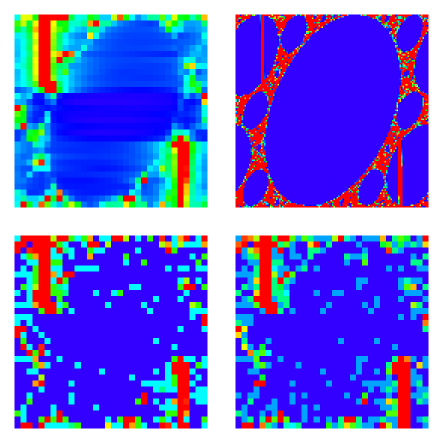
Figure 5: (color) Left: coarse grained diagram of $S^{(g)}$ for the sound signal $s^{\prime}_{n}$ obtained from the quantum computation (1) of the wavefunction after $t=100$ map iterations, top panel shows exact distribution $S^{(g)}$ and bottom panel is for a number of measurements as in Figs. 1,2. Bottom right: same as bottom left but with noise amplitude $\epsilon=0.05$ in the quantum gates. Right top: the exact Husimi distribution $h(l,\theta)$. The initial state is a momentum eigenstate at $l=100-N/2$. The color and axes are as in Fig. 2.

A more detailed analysis of the quantum sound $s^{\prime}_{n}$ can be obtained from the coarse grained spectrum digram similar to the one in Fig. 2. The coarse graining of $S_{k,j}$ is done by measuring 5 most significant and 5 less significant qubits corresponding to $a_{1}a_{2}...a_{5}$ and $a_{10}a_{11}...a_{14}$ that gives coarse grained distribution $S^{(g)}$ in $32\times 32$ cells. The diagrams of $S^{(g)}$ obtained for infinite and finite number of measurements are displayed in Fig. 5 (left top and bottom respectively). The exact diagram shows an interesting structure which is recovered with a finite number of measurements. This structure remains robust against noise in the quantum gates used for computation of $100$ map iterations and final QFT (Fig. 5 right bottom).

The origin of this structure becomes clear after its comparison with the coarse grained Wigner function called the Husimi distribution $h(\theta,l)$ levi ; husimi which is shown in Fig. 5 (right top) which is very close to $S^{(g)}$ (left top). Indeed, $h(\theta,l)$ is defined in the phase space $(l,\theta)$ by

$$h(l,\theta)=\sum_{l^{\prime}=l-N/2}^{l+N/2}G(l^{\prime}-l)\psi(l^{\prime})e^{il^{\prime}\theta}$$ (2)

where the gaussian smoothing function is $G(l^{\prime}-l)=(T/\pi)^{1/4}e^{-T(l^{\prime}-l)^{2}/2}/\sqrt{N}$ levi ; husimi . The Husimi distribution is always positive and gives a direct comparison between the classical phase space Liouville density distribution and a quantum wavefunction. In fact the coarse grained distribution $S^{(g)}$ is also given by equation (2) where $G(l^{\prime})$ is replaced by a constant in the interval $\Delta l^{\prime}=2^{5}$ and zero outside that corresponds to the application of QFT to less significant qubits $n_{f}=5$. Such a replacement modifies the values of coarse grained $h(\theta,l)$ but this modification remains small if $\Delta l^{\prime}\gg 1$ frahm . As a result we may argue that the signal $s^{\prime}_{n}$ represents the quantum sound of coarse grained Wigner function.

In conclusion, our results show that sound signals stored in a quantum memory can be reliably recognized and recovered on realistic quantum computers. The method proposed allows to obtain sound of quantum wavefunctions that can be useful for future quantum telecommunications.

This work was supported in part by the EC IST-FET project EDIQIP and the NSA and ARDA under ARO contract No. DAAD19-01-1-0553.

References

- (1) http://www.mpeg.org/MPEG/audio.html
- (2) M.A. Nielsen and I.L. Chuang Quantum Computation and Quantum Information, Cambridge Univ. Press, Cambridge (2000).
- (3) N. Gisin, G. Ribordy, W. Tittel, and H. Zbinden, Rev. Mod. Phys. 74, 145 (2002).
- (4) P.W.Shor, in Proc. 35th Annual Symposium on Foundation of Computer Science, Ed. S.Goldwasser (IEEE Computer Society, Los Alamitos, CA, 1994), p.124.
- (5) Y.S. Weinstein, M.A. Pravia, E.M. Fortunato, S. Lloyd, and D.G. Cory, Phys. Rev. Lett. 86, 1889 (2001).
- (6) L.M.K.Vandersypen, M. Steffen, G. Breyta, C.S. Yannoni, M.H. Sherwood, and I.L. Chuang, Nature 414, 883 (2001).
- (7) S.Gulde, M.Riebe, G.P.T.Lancaster, C.Becher, J.Eschner, H.Häffner, F.Schmidt-Kaler, I.L.Chuang and R.Blatt, Nature 421, 48 (2003).
- (8) E. Wigner Phys. Rev. 40, 749 (1932); M. V. Berry, Phil. Trans. Royal Soc. 287, 237 (1977).
- (9) C. Miquel, J. P. Paz, M. Saraceno, E. Knill, R. Laflamme and C. Negrevergne, Nature 418, 59 (2002).
- (10) B. Lévi, B. Georgeot and D.L. Shepelyansky, Phys. Rev. E 67, 046220 (2003).
- (11) Sound is available at http://www.palantir.net/cgi-bin/file.cgi?file=wav/hal9000.wav
- (12) http://www.quantware.ups-tlse.fr/qaudio/
- (13) B. Georgeot and D. L. Shepelyansky, Phys. Rev. Lett. 86, 2890 (2001).
- (14) G. Benenti, G. Casati, S. Montangero and D. L. Shepelyansky, Phys. Rev. Lett. 87, 227901 (2001).
- (15) S.-J. Chang and K.-J. Shi, Phys. Rev. A 34, 7 (1986).
- (16) Detailed analysis of quantum computation of Husimi distribution is done by K.M. Frahm (in preparation, 2003).