Optimal control theory for unitary transformations

Abstract

The dynamics of a quantum system driven by an external field is well described by a unitary transformation generated by a time dependent Hamiltonian. The inverse problem of finding the field that generates a specific unitary transformation is the subject of study. The unitary transformation which can represent an algorithm in a quantum computation is imposed on a subset of quantum states embedded in a larger Hilbert space. Optimal control theory (OCT) is used to solve the inversion problem irrespective of the initial input state. A unified formalism, based on the Krotov method is developed leading to a new scheme. The schemes are compared for the inversion of a two-qubit Fourier transform using as registers the vibrational levels of the $X^{1}\Sigma^{+}_{g}$ electronic state of Na₂. Raman-like transitions through the $A^{1}\Sigma^{+}_{u}$ electronic state induce the transitions. Light fields are found that are able to implement the Fourier transform within a picosecond time scale. Such fields can be obtained by pulse-shaping techniques of a femtosecond pulse. Out of the schemes studied the square modulus scheme converges fastest. A study of the implementation of the $Q$ qubit Fourier transform in the Na₂ molecule was carried out for up to 5 qubits. The classical computation effort required to obtain the algorithm with a given fidelity is estimated to scale exponentially with the number of levels. The observed moderate scaling of the pulse intensity with the number of qubits in the transformation is rationalized.

PACS number(s): 82.53.Kp 03.67.Lx 33.90.+h 32.80.Qk

I Introduction

Coherent control was initiated to steer a quantum system to a final objective via an external field RZ00 ; SB03 . If the initial and final objective states are pure, the method can be termed state-to-state coherent control. By generalizing, the problem of steering simultaneously a set of initial pure states to a set of final states can be formulated. Such a possibility has direct applicability in quantum computing where an algorithm implemented as a unitary transformation operating on a set of states has to be carried out irrespective of the input. In this application both input and output are encoded as a superposition of these states NC00 .

To implement such a control, the external driving field that induces a pre-specified unitary transformation has to be found. Different methods have been suggested for this task. Some rely on factorizing the algorithm encoded as a unitary transformation, to a set of elementary gates and then finding a control solution for the elementary unitary evolution of a single gate NC00 ; lloyd95 . The inherent difficulty in such an approach is that in general the field addresses many levels simultaneously. Therefore, when a particular single gate operation is carried out other levels are affected. This means that the ideal single gate unitary transformation has to be implemented so that all other possible transitions are avoided. The problem is simpler when each allowed transition is selectively addressable SGRR02 . However, in general the problem of undesired coupling has to be corrected. A specific solution has been suggested TL00 but a general solution is not known.

The presence of a large number of levels coupled to the external driving field is especially relevant in the implementation of quantum computing in molecular systems ZKLA01 ; AKL02 ; TKV01 . The use of optimal control theory (OCT) has been proposed as a possible solution TKV01 ; RB01 . In recent years OCT for quantum systems RZ00 has received considerable attention, leading to effective methods for obtaining the driving field which will induce a desired transition between preselected initial and final states. To address the control problem of inducing a particular unitary transformation the state-to-state OCT has to be augmented. For example, if the unitary transformation is to relate the initial states $|\varphi_{ik}\rangle$ with the final states $|\varphi_{fk}\rangle$, the state-to-state OCT derives an optimal field $\epsilon_{k}$ for each pair of initial and final states $(\varphi_{ik},\varphi_{fk})$. But the fields $\epsilon_{k}$ obtained are in general different, so that the evolution induced by $\epsilon_{k}$ is not appropriate for a different set of initial and final states. In order to implement a given unitary transformation a single field $\epsilon$ that relates simultaneously to all the relevant pairs $(\varphi_{ik},\varphi_{fk})$ is needed.

Two approaches have been suggested to generalize OCT for unitary transformations. The first approach is formulated directly on the evolution operator PK02 . An alternative approach uses the simultaneous optimization of several state-to-state transitions RB01 ; TV02 . The present paper develops a comprehensive framework for constructing an OCT solution for the unitary transformation. The study explores various approaches. A common framework for an iterative solution based on the Krotov approach TKO92 is developed. As a result, the numerical implementation of the methods are almost identical enabling an unbiased assessment. The implementation of the Fourier transform algorithm in a molecular environment is chosen as a case study. The performance of the various OCT schemes is compared in a realistic setup. A crucial demand in quantum computing is obtaining high fidelity of the solution. The present OCT scheme can be viewed as an iterative classical algorithm which finds a field that implements the quantum algorithm. The obvious questions are:

• What are the computational resources required to obtain a high fidelity result?

• How do these computational resources scale with the number of qubits in the quantum algorithm?

• How do the actual physical resources i.e. the integrated power of the field scale with the number of qubits in the quantum algorithm?

The paper is organized as follow: In Sec. II the problem is formulated introducing different objectives devoted to the optimization of a given unitary transformation. In Sec. III the application of the Krotov method of optimization of the given objectives is described. Expressions obtained for the optimal field are formulated as well as the implementation of the method. The variational method to derive the optimization equations is commented on in Appendix A. The results are used to study the implementation of a unitary transformation in a molecular model Sec. IV. Finally, in Sec. V results are discussed.

II Implementation of a unitary transformation

II.1 Description of the problem

The objective of the study is to devise a method to find the driving field that executes a unitary transformation on a subsystem embedded in a larger Hilbert space. The unitary transformation is to be applied in a Hilbert space $\cal M$ of dimension $M$, expanded by an orthonormal basis of states $\{|m\rangle\}$ ($m=1,...,M$). The selected unitary transformation is imposed on the subspace $\cal N$ of $N$ levels of the system ($N\leq M$). In the context of quantum computation, the $N$ levels correspond to the physical implementation of the qubit(s) embedded in a larger system. The additional levels ($m=N+1,...,M$), considered as “spurious levels”, are only indirectly involved in the target unitary transformation.

In any realistic implementation of quantum computing, ”spurious levels” always exist. One reason is that the system is never completely isolated from the environment. In addition, the control levers, that in the present case is the dipole operator, connects directly only part of the primary levels. An example is the implementation of quantum computation using rovibronic molecular levels. The transition dipole connects two electronic surfaces PK02 . The primary states reside on one surface, so that Raman-like transitions are used to implement the unitary transformation. The advantage of this setup is that the transitions frequencies between the electronic surfaces are in the visible region, for which the pulse shaping technology is well developed nelson . Other levels residing on both of the electronic surfaces become spurious in the sense that any leakage to them destroys the desired final result. However at intermediate times these levels constitute a temporary storage space which facilitates the execution of the transformation.

The objective is to implement a selected unitary transformation in the relevant subspace ${\cal N}$ at a given final time $T$. The target unitary transformation is represented by an operator in the Hilbert space of the primary system and is denoted by ${\boldsymbol{\mathrm{\widehat{O}}}}$. For $N<M$, the matrix representation of ${\boldsymbol{\mathrm{\widehat{O}}}}$ in the basis $\{|m\rangle\}$ has two blocks of dimension $N\times N$ and $(M-N)\times(M-N)$. The elements connecting these blocks are zero. This structure means that population is not transferred between the two subspaces at the target time $T$, but can take place at intermediate times. Only the $N\times N$ block is relevant for the optimization procedure, while the other remains arbitrary.

The dynamics of the system is generated by the Hamiltonian ${\boldsymbol{\mathrm{\widehat{H}}}}$,

$${\boldsymbol{\mathrm{\widehat{H}}}}(\epsilon)={\boldsymbol{\mathrm{\widehat{H}}}}_{0}-{\boldsymbol{\mathrm{\widehat{\mu}}}}\,\epsilon(t)\,,$$ (1)

where ${\boldsymbol{\mathrm{\widehat{H}}}}_{0}$ is the free Hamiltonian, $\epsilon(t)$ is the driving field and ${\boldsymbol{\mathrm{\widehat{\mu}}}}$ is a system operator describing the coupling between system and field. In the molecular systems, this coupling corresponds to the transition dipole operator and the driving field becomes radiation. In some cases more than one independent driving field can be considered. An example is when two components of the polarization of an electro-magnetic field are separately controlled BG01 . The generalization of the formalism in such a case is straightforward.

The system dynamics is fully specified by the evolution operator ${\boldsymbol{\mathrm{\widehat{U}}}}(t,0;\epsilon)$. An optimal field $\epsilon_{opt}$ induces the target unitary transformation ${\boldsymbol{\mathrm{\widehat{O}}}}$ at time $T$ when

$${\boldsymbol{\mathrm{\widehat{U}}}}(T,0;\epsilon_{opt})\,=\,e^{-i\phi(T)}\,{\boldsymbol{\mathrm{\widehat{O}}}}\,.$$ (2)

Eq. (2) implies a condition on only the $N\times N$ block of the matrix representation of ${\boldsymbol{\mathrm{\widehat{U}}}}$. The phase $\phi(T)$ is introduced to point out that the target unitary transformation ${\boldsymbol{\mathrm{\widehat{O}}}}$ can be implemented only up to an arbitrary global phase. The phase $\phi$ can be decomposed into two terms, $\phi_{1}(T)+\phi_{2}(T)$. The first, $\phi_{1}$, originates from the arbitrary choice of the origin of the energy levels. Formally, a term proportional to the identity operator can always be added to the Hamiltonian. When the states $|m\rangle$ correspond to the eigenstates of ${\boldsymbol{\mathrm{\widehat{H}}}}_{0}$, the phase $\phi_{1}$ is

$$\phi_{1}(T)=\frac{\sum_{m=1}^{M}\,E_{m}\,T}{M\,\hbar}\,,$$ (3)

where $E_{m}$ is the energy of the level $m$. The phase $\phi_{2}$ reflects the arbitrariness of the unitary transformation for the levels $m=N+1,...,M$ which are not part of the target.

The method to determine the optimal field is based on maximizing a real functional of the field that depends on both the target unitary transformation and the evolution generated by the Hamiltonian, fulfilling Eq. (2). The problem of unitary transformation optimization is then reduced to a functional optimization. However different formulations of the problem can be made, leading to different functionals and then, in principle to different results. In the present context two different formulations have been proposed, one based on the evolution operator PK02 and the other on simultaneous $N$ state to state transitions TV02 . These formulations are closely related. A similar optimization procedure is described in Sec. III.

II.2 Evolution operator formulation

The optimization formulation is based on the definition of a complex functional $\tau$ that depends on the evolution operator at time $T$ PK02 . The following functional is introduced:

$$\tau({\boldsymbol{\mathrm{\widehat{O}}}};T;\epsilon)={\rm Tr}\{{\boldsymbol{\mathrm{\widehat{O}}}}^{\dagger}{\boldsymbol{\mathrm{\widehat{U}}}}(T,0;\epsilon){\boldsymbol{\mathrm{\widehat{P}}}}_{N}\}\,=\sum_{n=1}^{N}\langle n|{\boldsymbol{\mathrm{\widehat{O}}}}^{\dagger}{\boldsymbol{\mathrm{\widehat{U}}}}(T,0;\epsilon)|n\rangle\,,$$ (4)

where the projection ${\boldsymbol{\mathrm{\widehat{P}}}}_{N}=\sum_{n=1}^{N}\,|n\rangle\langle n|$ is used. $\{|n\rangle\}$ denotes an orthonormal basis of the subspace $\cal N$. As ${\boldsymbol{\mathrm{\widehat{O}}}}$ is a unitary transformation in the relevant subspace, the functional $\tau$ is a complex number restricted to the interior of a circle in the complex plane of radius $N$ centered at the origin. The modulus of $\tau$ is equal to $N$ only for an optimal field fulfilling Eq. (2). $\tau$ can then be interpreted as an indicator of the fidelity of the implementation on the target unitary transformation PK02 . When $\tau$ approaches $N$, the transformation imposed by the field converges to the target objective.

Since $\tau$ is complex, several different real functionals can be associated with it. In Ref. PK02 the optimization of the real part of $\tau$, or the imaginary part, or a linear combination of both was suggested to find the optimal field. It was found that all these possibilities show a similar performance. For this reason, the present paper employs the optimization of the real part chosen as a representative case. The functional is therefore defined as:

$$F_{re}=-{\rm Re}\left[\tau({\boldsymbol{\mathrm{\widehat{O}}}};T;\epsilon)\right]=-{\rm Re}\left[\sum_{n=1}^{N}\langle n|{\boldsymbol{\mathrm{\widehat{O}}}}^{\dagger}{\boldsymbol{\mathrm{\widehat{U}}}}(T,0;\epsilon)|n\rangle\right]\,.$$ (5)

The functional reaches its minimum value, $F_{re}=-N$, when the driving field induces the target unitary transformation but however with the additional condition that the phase term $\exp(-i\phi(T))$ is equal to one.

Other functionals based on $\tau$ but without any condition on the phase can be defined. In this work the squared modulus of $\tau$ with a negative sign is studied:

$$F_{sm}=-|\tau({\boldsymbol{\mathrm{\widehat{O}}}};T;\epsilon)|^{2}=-\sum_{n=1}^{N}\sum_{n^{\prime}=1}^{N}\langle n|{\boldsymbol{\mathrm{\widehat{O}}}}^{\dagger}{\boldsymbol{\mathrm{\widehat{U}}}}(T,0;\epsilon)|n\rangle\,\langle n^{\prime}|{\boldsymbol{\mathrm{\widehat{U}}}}(T,0;\epsilon)^{\dagger}{\boldsymbol{\mathrm{\widehat{O}}}}|n^{\prime}\rangle\,,$$ (6)

with minimum value $F_{sm}=-N^{2}$ for any field satisfying Eq. (2).

II.3 Formulation of the Simultaneous $N$ state to state transitions

This formulation is based on the simultaneous optimization of $N$ transitions between a set of initial states $|l\rangle$ and the corresponding final states ${\boldsymbol{\mathrm{\widehat{O}}}}|l\rangle$ ($l=1,\dots,N$) TV02 . For this purpose the following functional is defined,

$$\eta({\boldsymbol{\mathrm{\widehat{O}}}};T;\epsilon)={\rm Tr}\left\{\sum_{l=1}^{N}{\boldsymbol{\mathrm{\widehat{O}}}}^{\dagger}{\boldsymbol{\mathrm{\widehat{U}}}}(T,0;\epsilon)|l\rangle\,\langle\l|{\boldsymbol{\mathrm{\widehat{U}}}}(T,0;\epsilon)^{\dagger}{\boldsymbol{\mathrm{\widehat{O}}}}|l\rangle\,\langle\l|\right\}=\sum_{l=1}^{N}|\langle l|{\boldsymbol{\mathrm{\widehat{O}}}}^{\dagger}{\boldsymbol{\mathrm{\widehat{U}}}}(T,0;\epsilon)|l\rangle|^{2}\,.$$ (7)

Notice that while $\tau$ is defined as the sum of amplitudes, $\eta$ is defined as the sum of overlaps at the final time $T$. The parameter $\eta$ is a positive real number and its maximum value, $N$, is reached when all the initial states $|l\rangle$ are driven by the field to the final target states ${\boldsymbol{\mathrm{\widehat{O}}}}|l\rangle$, except for a possible arbitrary phase associated with each transition. The arbitrariness of these phases implies that the set of initial states $|l\rangle$ must be chosen carefully. In order to account for all the possible transitions, the states $|l\rangle$ have to faithfully represent all the relevant subspace $\cal N$ i.e. constitute a complete basis set. However, a choice of an orthonormal basis could produce undesired results. For example, the ambiguity of using an orthonormal basis $\{|n\rangle\}$ in the relevant subspace and an arbitrary unitary transformation ${\boldsymbol{\mathrm{\widehat{D}}}}$, diagonal in that basis. The product ${\boldsymbol{\mathrm{\widehat{O}}}}\,{\boldsymbol{\mathrm{\widehat{D}}}}$ will also be a unitary transformation. If $\epsilon_{O}$ and $\epsilon_{OD}$ are fields that generate ${\boldsymbol{\mathrm{\widehat{O}}}}$ and ${\boldsymbol{\mathrm{\widehat{O}}}}\,{\boldsymbol{\mathrm{\widehat{D}}}}$ at time $T$ respectively, they both will have the same fidelity $\eta$,

$$\eta_{\perp}({\boldsymbol{\mathrm{\widehat{O}}}};T;\epsilon_{O})=\eta_{\perp}({\boldsymbol{\mathrm{\widehat{O}}}};T;\epsilon_{OD})\,,$$ (8)

where $\perp$ denotes that $\eta$ was evaluated using an orthonormal basis. Then any algorithm based on optimizing $\eta$ that uses an orthonormal basis could find a solution for the field corresponding to the implementation of an arbitrary unitary transformations of the form ${\boldsymbol{\mathrm{\widehat{O}}}}\,{\boldsymbol{\mathrm{\widehat{D}}}}$. (${\boldsymbol{\mathrm{\widehat{O}}}}$ is a particular case when ${\boldsymbol{\mathrm{\widehat{D}}}}$ is the identity operator). The reason for this discrepancy is that $\eta$ is only sensitive to the overlap of each pair of initial $|l\rangle$ and final ${\boldsymbol{\mathrm{\widehat{O}}}}|l\rangle$ states, leaving undetermined the relative phases between them. For the optimization procedure to succeed a careful choice of the initial set of states is necessary. A simple solution is to compose the last $N$ state as a superposition of all states in the basis $\sum_{l=1}^{N}|n\rangle/\sqrt{N}$, and to keep as is the first $N-1$ states of an orthonormal basis. For this set of states, the maximum condition is achieved only when the field induces the target unitary transformation up to a possible global phase.

To summarize the functional $-\eta$ in is used,

$$F_{ss}=-\eta({\boldsymbol{\mathrm{\widehat{O}}}};T;\epsilon),$$ (9)

with a minimum value $F_{ss}=-N$. The optimal field reached satisfies Eq. (2), subject to a choice of the set of states $|l\rangle$ which determines the relative phases.

II.4 Initial to final state optimization

The present formulations of quantum control assume that the target unitary transformation ${\boldsymbol{\mathrm{\widehat{O}}}}$ is explicitly known, at least in the subspace $\cal N$. In most previous applications of optimal control theory, the objective was specified as the maximization of the expectation value of a given observable at time $T$ subject to a predefined initial state RZ00 . Both mixed and pure initial states were considered BKT01 ; Ohtsuki03 . A particular case is the determination of an optimal field to drive the system from a given pure initial state $|\varphi_{i}\rangle$ to a target pure final state $|\varphi_{f}\rangle$ at time $T$. This state-to-state objective optimization can be derived from the present formulation if the target unitary transformation becomes ${\boldsymbol{\mathrm{\widehat{O}}}}|\varphi_{i}\rangle=|\varphi_{f}\rangle$. The evolution operator formulation is then obtained by setting the projector ${\boldsymbol{\mathrm{\widehat{P}}}}_{N}=|\varphi_{i}\rangle\langle\varphi_{i}|$ in Eq. (4), obtaining the functional $\tau$,

$$\tau(\varphi_{i},\varphi_{f};T;\epsilon)\,=\,\langle\varphi_{f}|{\boldsymbol{\mathrm{\widehat{U}}}}(T,0;\epsilon)|\varphi_{i}\rangle\,.$$ (10)

The real functionals $F_{re}=-{\rm Re}[\tau]$ and $F_{sm}=-|\tau|^{2}$ are to be used in the study. As only a state-to-state transition is involved, the formulation is obtained by choosing $|l\rangle\equiv|\varphi_{i}\rangle$. In this case $\eta=|\tau|^{2}$ and $F_{ss}=F_{sm}$. Notice that this result is valid only when there is a single term in the sum in Eq. (4) and in Eq. (7).

III Optimization

A common optimization procedure for all the functionals $F$ as defined in the previous section is developed. The notation $|n\rangle$ for the states and $n$ its index will be used in the evolution operator formulation. The notation $|l\rangle$ and $l$ will be used in the simultaneous $N$ state to state transitions formulation. The notation $|\varphi_{ik}\rangle$ and $k$ where $k=1,\dots,N$, will be used when the results are valid for both cases. An evaluation of any of the functionals requires the knowledge of the states $|\varphi_{k}(T)\rangle={\boldsymbol{\mathrm{\widehat{U}}}}(T,0;\epsilon)|\varphi_{ik}\rangle$ and $|\varphi_{fk}\rangle={\boldsymbol{\mathrm{\widehat{O}}}}|\varphi_{ik}\rangle$. The operation of the evolution equation ${\boldsymbol{\mathrm{\widehat{U}}}}(t,0;\epsilon)|\varphi_{ik}\rangle$ can be calculated by solving the time-dependent Schrödinger equation

$$\frac{d}{dt}|\varphi_{k}(t)\rangle\,=\,-\frac{i}{\hbar}{\boldsymbol{\mathrm{\widehat{H}}}}(\epsilon)|\varphi_{k}(t)\rangle\,,$$ (11)

with an initial condition $|\varphi_{k}(0)\rangle=|\varphi_{ik}\rangle$. Since ${\boldsymbol{\mathrm{\widehat{H}}}}={\boldsymbol{\mathrm{\widehat{H}}}}(\epsilon)$ the state evolution will depend on the particular field. An alternative to Eq. (11) is the evolution equation for the unitary transformation itself PK02 .

The method of optimization depends on the availability of the states of the system $|\varphi_{k}(t)\rangle$ at intermediate times $0<t<T$.

Experimental realizations of OCT are typical examples where only initial and final knowledge of the states exist. For such cases feedback control and evolutionary methods are effective RZ00 . Such methods however require a large number of iterations to achieve convergence. A simulation of such a process requires repeated propagation of the $N$ states by the Schrödinger equation. Thus they are computationally intensive.

Computationally more effective methods are based on the knowledge of the states $|\varphi_{k}(t)\rangle$ at intermediate times. Additional constrains on the evolution are included that allow a modification of the field at intermediate times consistent with the improvement of the objective at the target time $T$. Some examples are the local-in-time optimization method BKT93 ; Sugawara03 , the conjugate gradient search method KRGT89 , the Krotov method TKO92 , and the variational approach PDR88 ; ZBR98 . A review of these common methods can be found in Ref. RZ00 . In the present study the Krotov method has been adopted. A brief description of the alternative variational method is given in Appendix A.

III.1 Krotov method of optimization

The Krotov method is utilized to derive an iterative algorithm to minimize a given functional that depends on both final and intermediate times Cf. Ref. ST02 .

For convenience, the equations are stated using real functions: $\alpha_{km}(t)\,\equiv\,{\rm Re}[\langle m|\varphi_{k}(t)\rangle]$ and $\beta_{km}(t)\,\equiv\,{\rm Im}[\langle m|\varphi_{k}(t)\rangle]$. The notation $\boldsymbol{\alpha}_{k}$ and $\boldsymbol{\beta}_{k}$ is used to describe the $M$-dimensional vectors with components $\alpha_{km}$ and $\beta_{km}$. Using such a notation, the evolution equation (11) becomes:

$$\frac{d}{dt}\boldsymbol{\alpha}_{k}(t)\, = \,\boldsymbol{\Omega}_{R}(t,\epsilon)\cdot\boldsymbol{\alpha}_{k}(t)\,-\,\boldsymbol{\Omega}_{I}(t,\epsilon)\cdot\boldsymbol{\beta}_{k}(t)\,,$$

$$\frac{d}{dt}\boldsymbol{\beta}_{k}(t)\, = \,\boldsymbol{\Omega}_{I}(t,\epsilon)\cdot\boldsymbol{\alpha}_{k}(t)\,+\,\boldsymbol{\Omega}_{R}(t,\epsilon)\cdot\boldsymbol{\beta}_{k}(t)\,,$$ (12)

where $\boldsymbol{\Omega}_{R}$ and $\boldsymbol{\Omega}_{I}$ are real matrices with the corresponding components composed of the real and imaginary parts of $\boldsymbol{\Omega}_{ij}=\langle i|(-i{\boldsymbol{\mathrm{\widehat{H}}}}/\hbar)|j\rangle$ where $|i\rangle$ and $|j\rangle$ are states from the basis set $\{|m\rangle\}$. The initial conditions are given by the vectors $\boldsymbol{\alpha}_{k}(0)$ and $\boldsymbol{\beta}_{k}(0)$ with components composed of the real and imaginary part of the amplitudes $\langle m|\varphi_{ik}\rangle$. $\boldsymbol{\alpha}_{fk}$ and $\boldsymbol{\beta}_{fk}$ denote the vectors corresponding to the amplitudes $\langle m|\varphi_{fk}\rangle$.

The formalism considers $\boldsymbol{\alpha}_{k}$, $\boldsymbol{\beta}_{k}$, and the field $\epsilon$ to be independent variables. A necessary consistency between them will be required in the final step of the algorithm. The vectors $\boldsymbol{f}_{\alpha}$ and $\boldsymbol{f}_{\beta}$ constitute the right hand side of Eq. (III.1),

$$\boldsymbol{f}_{\alpha}(t,\boldsymbol{\alpha}_{k},\boldsymbol{\beta}_{k},\epsilon)\,\equiv\,\boldsymbol{\Omega}_{R}(t,\epsilon)\cdot\boldsymbol{\alpha}_{k}(t)\,-\,\boldsymbol{\Omega}_{I}(t,\epsilon)\cdot\boldsymbol{\beta}_{k}(t)\,,$$

$$\boldsymbol{f}_{\beta}(t,\boldsymbol{\alpha}_{k},\boldsymbol{\beta}_{k},\epsilon)\,\equiv\,\boldsymbol{\Omega}_{I}(t,\epsilon)\cdot\boldsymbol{\alpha}_{k}(t)\,+\,\boldsymbol{\Omega}_{R}(t,\epsilon)\cdot\boldsymbol{\beta}_{k}(t)\,.$$ (13)

The vectors $\boldsymbol{f}_{\alpha}$ ($\boldsymbol{f}_{\beta}$) are equal to the total time derivative of $\boldsymbol{\alpha}$ ($\boldsymbol{\beta}$) only when the state is consistent with the field through the evolution equation (III.1). The dependence of $\boldsymbol{\alpha}$ and $\boldsymbol{\beta}$ on $t$ will be made explicit only when necessary. An important property of the problems under study is that $\boldsymbol{f}_{\alpha}$ and $\boldsymbol{f}_{\beta}$ are linear in the functions $\{\boldsymbol{\alpha},\boldsymbol{\beta}\}$ and $\epsilon$. This choice simplifies the optimization problem, the non-linear case has been studied in Ref. ST02 .

A “process” $w=w[t,\{\boldsymbol{\alpha},\boldsymbol{\beta}\},\epsilon]$ is defined as the set $\{\boldsymbol{\alpha},\boldsymbol{\beta}\}$ of $N$ vectors $\boldsymbol{\alpha}_{k}$ and $N$ vectors $\boldsymbol{\beta}_{k}$ related to the field $\epsilon$ through the evolution equations with the initial conditions $\boldsymbol{\alpha}_{k}(0)$ and $\boldsymbol{\beta}_{k}(0)$. A functional of the process can be defined:

$$J[w]\,=\,F(\{\boldsymbol{\alpha}(T),\boldsymbol{\beta}(T)\})\,+\,\int_{0}^{T}g(\epsilon)\,dt\,.$$ (14)

For the present applications $F$ can be any of the functionals $F_{re}$, $F_{sm}$, $F_{ss}$ as introduced in the section II. The optimal field is found by a minimization of the functional $J$. The integral term represents additional constrains originating from the evolution equation of the system. For simplicity only the case where $g$ is a function of the field $\epsilon$ is presented, but a generalization to a more general case in which $g$ depends on $\boldsymbol{\alpha}(t)$ and $\boldsymbol{\beta}(t)$ is straightforward. The particular dependence of $g$ on the field will be discussed later.

The main idea in the Krotov method is to introduce a new functional that mixes the separated dependence on intermediate and final times in the original functional (14). Using the new functional it is possible to derive an iterative procedure that modifies the field at intermediate times in a consistent way with the minimization of $F$ at time $T$. The new functional is defined as

$$L[w,\Phi]\,=\,G(\{\boldsymbol{\alpha}(T),\boldsymbol{\beta}(T)\})\,-\,\Phi(0,\{\boldsymbol{\alpha}(0),\boldsymbol{\beta}(0)\})\,-\,\int_{0}^{T}R(t,\{\boldsymbol{\alpha},\boldsymbol{\beta}\},\epsilon)\,dt\,,$$ (15)

where,

$$G(\{\boldsymbol{\alpha}(T),\boldsymbol{\beta}(T)\})\,=\,F(\{\boldsymbol{\alpha}(T),\boldsymbol{\beta}(T)\})\,+\,\Phi(T,\{\boldsymbol{\alpha}(T),\boldsymbol{\beta}(T)\})\,,$$ (16)

and

$$R(t,\{\boldsymbol{\alpha},\boldsymbol{\beta}\},\epsilon)\, = \,-g(\epsilon)\,+\,\frac{\partial\Phi}{\partial t}(t,\{\boldsymbol{\alpha},\boldsymbol{\beta}\})$$

$$+ \,\sum_{k=1}^{N}\,\boldsymbol{\frac{\partial\Phi}{\partial\alpha_{k}}}(t,\{\boldsymbol{\alpha},\boldsymbol{\beta}\})\cdot\boldsymbol{f}_{\alpha}(t,\boldsymbol{\alpha}_{k},\boldsymbol{\beta}_{k},\epsilon)$$

$$+ \,\sum_{k=1}^{N}\,\boldsymbol{\frac{\partial\Phi}{\partial\beta_{k}}}(t,\{\boldsymbol{\alpha},\boldsymbol{\beta}\})\cdot\boldsymbol{f}_{\beta}(t,\boldsymbol{\alpha}_{k},\boldsymbol{\beta}_{k},\epsilon)\,.$$ (17)

$\Phi(t,\{\boldsymbol{\alpha},\boldsymbol{\beta}\})$ denotes an arbitrary continuously differentiable function. The partial derivatives of $\Phi$, $\boldsymbol{\frac{\partial\Phi}{\partial\alpha_{k}}}$ and $\boldsymbol{\frac{\partial\Phi}{\partial\beta_{k}}}$, form a vector with $m$ components. In the following $t$, $\boldsymbol{\alpha}$ and $\boldsymbol{\beta}$ are considered to be independent variables in $\Phi$.

When $\{\boldsymbol{\alpha},\boldsymbol{\beta}\}$ and the field are related by Eq. (III.1), $R$ can be written as $R=-g+d\Phi/dt$. Introducing this result in Eq. (15), it can be shown ST02 that for any scalar function $\Phi$ and any process $w$, $L[w,\Phi]=J[w]$. Then the minimization of $J$ is completely equivalent to the minimization of $L$.

III.1.1 Iterative algorithm to minimize $L$

The advantage of the definition of the functional $L[w]$ is the complete freedom in the choice of $\Phi$. This property is used to derive from an arbitrary process $w^{(0)}[t,\{\boldsymbol{\alpha}^{(0)},\boldsymbol{\beta}^{(0)}\},\epsilon^{(0)}]$ a new process $w^{(1)}[t,\{\boldsymbol{\alpha}^{(1)},\boldsymbol{\beta}^{(1)}\},\epsilon^{(1)}]$ such that $L[w^{(1)},\Phi]\leq L[w^{(0)},\Phi]$. The procedure can be summarized as follows:

• (i) $\Phi$ is constructed so that the functional $L[w^{(0)}]$ is a maximum with respect to any possible choice of the set $\{\boldsymbol{\alpha},\boldsymbol{\beta}\}$. This condition gives a complete freedom to change $\epsilon$. The related changes of the states are consistent with the system evolution, Eq. (III.1), and therefore, will not interfere with the the minimization of $L$.

• (ii) A new field $\epsilon^{(1)}$ is derived with the condition of maximizing $R$, decreasing then the value of $L$ with respect to the process $w^{(0)}$. In this step the consistency between the new field and the new states of the system $\{\boldsymbol{\alpha}^{(1)},\boldsymbol{\beta}^{(1)}\}$ must be maintained.

The new field $\epsilon^{(1)}$ becomes the starting point of a new iteration, and steps (i) and (ii) are repeated until the desired convergence is achieved.

III.1.2 The linear problem: construction of $\Phi$ to first order

The difficult task in the Krotov method is the construction of $\Phi$ so that $L$ is maximum for $\{\boldsymbol{\alpha}^{(0)},\boldsymbol{\beta}^{(0)}\}$. The maximum condition on $L$ is equivalent to imposing a maximum on $G$ and a minimum on $R$. However, in some cases the maximum and minimum conditions can be relaxed to extreme conditions for $G$ and $R$, which simplifies the problem.

The extreme conditions for $R$ with respect to $\{\boldsymbol{\alpha}^{(0)},\boldsymbol{\beta}^{(0)}\}$ are given by

$$\boldsymbol{\frac{\partial R}{\partial\alpha_{k}}}(t,\{\boldsymbol{\alpha}^{(0)},\boldsymbol{\beta}^{(0)}\},\epsilon^{(0)}) = 0\,,$$

$$\boldsymbol{\frac{\partial R}{\partial\beta_{k}}}(t,\{\boldsymbol{\alpha}^{(0)},\boldsymbol{\beta}^{(0)}\},\epsilon^{(0)}) = 0\,.$$ (18)

The following vectors are introduced

$$\boldsymbol{\gamma}_{k}(t)\, = \,\boldsymbol{\frac{\partial\Phi}{\partial\alpha_{k}}}(t,\{\boldsymbol{\alpha}^{(0)},\boldsymbol{\beta}^{(0)}\})\,,$$

$$\boldsymbol{\delta}_{k}(t)\, = \,\boldsymbol{\frac{\partial\Phi}{\partial\beta_{k}}}(t,\{\boldsymbol{\alpha}^{(0)},\boldsymbol{\beta}^{(0)}\})\,.$$ (19)

$\boldsymbol{\gamma}_{k}$ and $\boldsymbol{\delta}_{k}$ are only functions of $t$, as the partial derivatives are evaluated in the specific set $\{\boldsymbol{\alpha}^{(0)},\boldsymbol{\beta}^{(0)}\}$. Using Eq. (III.1) the extreme conditions can be written as

$$\frac{d}{dt}\,\boldsymbol{\gamma}_{k}(t) = \,-\boldsymbol{\Omega}_{R}^{T}(t,\epsilon^{(0)})\cdot\boldsymbol{\gamma}_{k}(t)\,-\,\boldsymbol{\Omega}_{I}^{T}(t,\epsilon^{(0)})\cdot\boldsymbol{\delta}_{k}(t)\,,$$

$$\frac{d}{dt}\,\boldsymbol{\delta}_{k}(t) = \,\boldsymbol{\Omega}_{I}^{T}(t,\epsilon^{(0)})\cdot\boldsymbol{\gamma}_{k}(t)\,-\,\boldsymbol{\Omega}_{R}^{T}(t,\epsilon^{(0)})\cdot\boldsymbol{\delta}_{k}(t)\,,$$ (20)

where $\boldsymbol{\Omega}^{T}$ denotes the transpose of the matrix $\boldsymbol{\Omega}$. The extreme conditions for $G$ are

$$\boldsymbol{\frac{\partial G}{\partial\alpha_{k}(T)}}(\{\boldsymbol{\alpha}^{(0)}(T),\boldsymbol{\beta}^{(0)}(T)\})\, = \,0\,,$$

$$\boldsymbol{\frac{\partial G}{\partial\beta_{k}(T)}}(\{\boldsymbol{\alpha}^{(0)}(T),\boldsymbol{\beta}^{(0)}(T)\})\, = \,0\,.$$ (21)

Using Eq. (16) and Eq. (III.1.2)

$$\boldsymbol{\gamma}_{k}(T)\, = \,-\boldsymbol{\frac{\partial F}{\partial\alpha_{k}(T)}}(\{\boldsymbol{\alpha}{(0)}(T),\boldsymbol{\beta}^{(0)}(T)\})\,,$$

$$\boldsymbol{\delta}_{k}(T)\, = \,-\boldsymbol{\frac{\partial F}{\partial\beta_{k}(T)}}(\{\boldsymbol{\alpha}^{(0)}(T),\boldsymbol{\beta}^{(0)}(T)\})\,.$$ (22)

The above conditions at time $T$, together with Eq. (III.1.2) determine completely the set $\{\boldsymbol{\gamma}(t),\boldsymbol{\delta}(t)\}$. As they are defined as the partial derivative of $\Phi$ with respect to $\alpha_{km}$ and $\beta_{km}$, $\Phi$ is expanded to first order (denoted as $\Phi^{\star}$),

$$\Phi^{\star}(t,\{\boldsymbol{\alpha},\boldsymbol{\beta}\})\,=\,\sum_{k=1}^{N}\,\left[\boldsymbol{\gamma}_{k}(t)\cdot\boldsymbol{\alpha}_{k}(t)\,+\,\boldsymbol{\delta}_{k}(t)\cdot\boldsymbol{\beta}_{k}(t)\right]\,.$$ (23)

By employing $\Phi^{\star}$, the functions $G^{\star}$ and $R^{\star}$ can also be constructed to first order using Eq. (16) and (III.1) respectively. This completes the first step in the iterative algorithm.

To accomplish the second step $R$ is maximized with respect to the field. Again in some cases the maximum condition can be relaxed to the extreme condition $\partial R/\partial\epsilon=0$. Using the expression for $R^{\star}$ leads to

$$\frac{\partial g}{\partial\epsilon}(\epsilon^{(1)})\, = \,\sum_{k=1}^{N}\,\boldsymbol{\gamma}_{k}(t)\cdot\frac{\partial\boldsymbol{f}_{\alpha}}{\partial\epsilon}(t,\boldsymbol{\alpha}_{k}^{(1)},\boldsymbol{\beta}_{k}^{(1)},\epsilon^{(1)})$$

$$+ \,\sum_{k=1}^{N}\,\boldsymbol{\delta}_{k}(t)\cdot\frac{\partial\boldsymbol{f}_{\beta}}{\partial\epsilon}(t,\boldsymbol{\alpha}_{k}^{(1)},\boldsymbol{\beta}_{k}^{(1)},\epsilon^{(1)})\,.$$ (24)

Eq. (III.1.2) is used to derive the new field $\epsilon^{(1)}$ in each iteration. This equation must be solved in a consistent way with Eq. (III.1) describing the system dynamics.

Due to the use of extreme instead of maximum or minimum conditions, it must be checked that the new process, $w^{(1)}$, improves the original objective in each iteration $J[w^{(0)}]-J[w^{(1)}]\geq 0$:

$$J[w^{(0)}]-J[w^{(1)}]\,=\,L[w^{(0)},\Phi^{\star}]-L[w^{(1)},\Phi^{\star}]\,=\,\Delta_{1}\,+\,\int_{0}^{T}\Delta_{2}(t)\,dt\,.$$ (25)

where,

$$\Delta_{1}\,=\,G^{\star}(\{\boldsymbol{\alpha}^{(0)}(T),\boldsymbol{\beta}^{(0)}(T)\})\,-\,G^{\star}(\{\boldsymbol{\alpha}^{(1)}(T),\boldsymbol{\beta}^{(1)}(T)\})\,.$$ (26)

$$\Delta_{2}(t)\,=\,R^{\star}(t,\{\boldsymbol{\alpha}^{(1)},\boldsymbol{\beta}^{(1)}\},\epsilon^{(1)})\,-\,R^{\star}(t,\{\boldsymbol{\alpha}^{(1)},\boldsymbol{\beta}^{(1)}\},\epsilon^{(0)})\,.$$ (27)

The above relation is obtained when $\boldsymbol{f}_{\alpha}$ and $\boldsymbol{f}_{\beta}$ are linear in $\{\boldsymbol{\alpha},\boldsymbol{\beta}\}$

$$R^{\star}(t,\{\boldsymbol{\alpha},\boldsymbol{\beta}\},\epsilon^{(0)})\,=\,-\,g(t,\epsilon^{(0)})\,,$$ (28)

for any value of $\{\boldsymbol{\alpha},\boldsymbol{\beta}\}$.

A sufficient condition for $J[w^{(0)}]-J[w^{(1)}]\geq 0$ is $\Delta_{1},\Delta_{2}(t)\geq 0$. $\Delta_{1}$ depends on the choice $F$ and $\Delta_{2}(t)$ on the choice of $g$ so that each case must be analyzed separately. These conditions imply that the Krotov iterative algorithm convergence monotonically to the final objective.

III.1.3 Dependence on $F$

The dependence of $G^{\star}$ on $F$ can be made explicit by introducing $\Phi^{\star}$ and using Eq. (23) and Eq. (16),

$$G^{\star}(\{\boldsymbol{\alpha}(T),\boldsymbol{\beta}(T)\})\, = \,F(\{\boldsymbol{\alpha}(T),\boldsymbol{\beta}(T)\})$$

$$- \,\sum_{k=1}^{N}\,\boldsymbol{\frac{\partial F}{\partial\alpha_{k}(T)}}\cdot\boldsymbol{\alpha}_{k}(T)\,\,+\,\boldsymbol{\frac{\partial F}{\partial\beta_{k}(T)}}\cdot\boldsymbol{\beta}_{k}(T)\,.$$ (29)

When $F$ is linear in $\{\boldsymbol{\alpha},\boldsymbol{\beta}\}$ $G^{\star}\equiv 0$ and then $\Delta_{1}\equiv 0$. In this case all the improvement towards the original objective in the iteration is due to the term $\Delta_{2}(t)$. When $F$ is non linear in $\{\boldsymbol{\alpha},\boldsymbol{\beta}\}$ the condition $\Delta_{1}\leq 0$ must be checked in each case.

An additional difficulty is that the conditions (III.1.2) for $\boldsymbol{\gamma}$ and $\boldsymbol{\delta}$ depend on the particular choice of $F$. In all the cases under study ($F_{re}$, $F_{sm}$ and $F_{ss}$)

$$\boldsymbol{\gamma}_{k}(T)\, = \,c_{k}\,\boldsymbol{\alpha}_{fk}(T)\,,$$

$$\boldsymbol{\delta}_{k}(T)\, = \,d_{k}\,\boldsymbol{\beta}_{fk}(T)\,,$$ (30)

where the coefficients $c_{k}$ and $d_{k}$ depend on the sets $\{\boldsymbol{\alpha}^{(0)}(T),\boldsymbol{\beta}^{(0)}(T)\}$ and $\{\boldsymbol{\alpha}_{f},\boldsymbol{\beta}_{f}\}$. Defining the vectors $\tilde{\boldsymbol{\gamma}}_{k}=c_{k}^{-1}\,\boldsymbol{\gamma}_{k}$ and $\tilde{\boldsymbol{\delta}}_{k}=d_{k}^{-1}\,\boldsymbol{\delta}_{k}$, the conditions (III.1.2) for all the cases under consideration are:

$$\tilde{\boldsymbol{\gamma}}_{k}(T)\, = \,\boldsymbol{\alpha}_{fk}(T)\,,$$

$$\tilde{\boldsymbol{\delta}}_{k}(T)\, = \,\boldsymbol{\beta}_{fk}(T)\,.$$ (31)

Their evolution is given by Eq. (III.1.2). Changing $\boldsymbol{\gamma}$ and $\boldsymbol{\delta}$ to $\tilde{\boldsymbol{\gamma}}$ and $\tilde{\boldsymbol{\delta}}$ Eq. (III.1.2) can be written as

$$\frac{\partial g}{\partial\epsilon}(\epsilon^{(1)})\, = \,\sum_{k=1}^{N}\,c_{k}\,\tilde{\boldsymbol{\gamma}}_{k}(t)\cdot\frac{\partial{\boldsymbol{f}}_{\alpha}}{\partial\epsilon}(t,\boldsymbol{\alpha}_{k}^{(1)},\boldsymbol{\beta}_{k}^{(1)},\epsilon^{(1)})$$

$$+ \,\sum_{k=1}^{N}\,d_{k}\,\tilde{\boldsymbol{\delta}}_{k}(t)\cdot\frac{\partial\boldsymbol{f}_{\beta}}{\partial\epsilon}(t,\boldsymbol{\alpha}_{k}^{(1)},\boldsymbol{\beta}_{k}^{(1)},\epsilon^{(1)})\,.$$ (32)

The different choices of $F$ imply different coefficients ($c_{k}$ and $d_{k}$) and a possible different set of initial $|\varphi_{ik}\rangle$ and final $|\varphi_{fk}\rangle$ states. Nevertheless, the iterative procedure is identical in all the cases.

III.1.4 Dependence on $g(\epsilon)$

A delicate point is the choice of the function $g(\epsilon)$ in $J[w]$. The time integral in the functional should be bounded from below, otherwise the the additional constraint will dominate over the original objective $F$ in the functional $J$. In addition $\Delta_{2}(t)\geq 0$ is required in order to guarantee the monotonic convergence of the optimization method.

A consequence of the linear dependence of $\boldsymbol{f}_{\alpha}$, $\boldsymbol{f}_{\beta}$ and Eq. (III.1.3) is that the function $R^{\star}$ for the new process $w^{(1)}$ has the simple form

$$R^{\star}(t,\{\boldsymbol{\alpha}^{(1)},\boldsymbol{\beta}^{(1)}\},\epsilon^{(1)})\,=\,-g(\epsilon)\,+\,\left(\epsilon^{(1)}-\epsilon^{(0)}\right)\,\frac{\partial g}{\partial\epsilon}(\epsilon^{(1)})\,.$$ (33)

Using this expression together with Eq. (28) leads to

$$\Delta_{2}(t)\,=\,-g(\epsilon^{(1)})+g(\epsilon^{(0)})\,+\,\left(\epsilon^{(1)}-\epsilon^{(0)}\right)\frac{\partial g}{\partial\epsilon}(\epsilon^{(1)})\,,$$ (34)

A choice of $g(\epsilon)$ fulfilling the previous requirements is

$$g(\epsilon)\,=\,\lambda(t)\,\left[\epsilon(t)\,-\,\tilde{\epsilon}(t)\right]^{2}\,,$$ (35)

where $\tilde{\epsilon}$ is a reference field and $\lambda(t)$ is a positive function of $t$. Using Eq. (34) and for any field $\tilde{\epsilon}$

$$\Delta_{2}(t)\,=\,\lambda(t)\,\left[\Delta\epsilon(t)\right]^{2}\,\,\geq\,0,$$ (36)

where $\Delta\epsilon(t)\equiv\epsilon^{(1)}(t)-\epsilon^{(0)}(t)$. The method therefore will converge monotonically. Using Eq. (III.1.3) and Eq. (35) the field in the new iteration becomes:

$$\epsilon^{(1)}(t)\, = \,\tilde{\epsilon}(t)\,+\,\frac{1}{2\lambda(t)}\,\sum_{k=1}^{N}\,\left\{c_{k}\,\tilde{\boldsymbol{\gamma}}_{k}(t)\cdot\frac{\partial\boldsymbol{f}_{\alpha}}{\partial\epsilon}(t,\boldsymbol{\alpha}_{k}^{(1)},\boldsymbol{\beta}_{k}^{(1)},\epsilon^{(1)})\right.$$

$$+ \,\left.d_{k}\,\tilde{\boldsymbol{\delta}}_{k}(t)\cdot\frac{\partial\boldsymbol{f}_{\beta}}{\partial\epsilon}(t,\boldsymbol{\alpha}_{k}^{(1)},\boldsymbol{\beta}_{k}^{(1)},\epsilon^{(1)})\right\}\,.$$ (37)

The result of the iterative algorithm depends strongly on the choices of the reference field $\tilde{\epsilon}$ and on the function $\lambda(t)$.

Two possible choices of $\tilde{\epsilon}$ are analyzed. The first, $\tilde{\epsilon}=0$, is the one commonly used in OCT applications RZ00 . In this case, the additional constraint in $J[w]$ has the physical meaning that the total energy of the field in the time interval $[0,T]$ is limited. This however presents a problem when the iterative procedure reaches the optimal field. The iterative method is found to reduce the total objective $J$ by reducing the total pulse energy, slowing and even spoiling the convergence to the original objective $F$. The usual remedy is to stop the iterative algorithm before this difficulty is reached. However, such a procedure could prevent the optimization algorithm from obtaining high fidelity.

A different possibility is $\tilde{\epsilon}=\epsilon^{(0)}$ can avoid this problem RB01 ; BKT01 ; ST02 . In this iterative algorithm $\epsilon^{(0)}$ must be interpreted as the field in the previous iteration. Now the additional constraint in $J[w]$ has the physical interpretation that the change of the pulse energy in each iteration is limited. When the iterative procedure approaches the optimal solution the change in the field vanishes. Therefore, the convergence to the original objective is guaranteed. In the rest of the study $\tilde{\epsilon}=\epsilon^{(0)}$ was chosen.

The function $\lambda(t)$ introduces the shape function $s(t)$ i.e. $\lambda(t)=\lambda_{0}/s(t)$. The purpose of $s(t)$ is to turn the field on and off smoothly at the boundaries of the interval SV99 . $\lambda_{0}$ is a scaling parameter which determines the optimization strategy. When $\lambda_{0}$ is small the additional constraint on the field in the functional becomes insignificant, resulting in large modifications in the field in each iteration. This is equivalent to a bold search strategy where large excursions in the functional space of the field take place with each iteration. Large values of $\lambda_{0}$ imply small modifications in the field in each iteration, slowing the convergence process. Using large values of $\lambda_{0}$ is a conservative search strategy which is advantageous when a good initial guess field can be found. A possible mixed strategy is to initially use a bold optimization with small values of $\lambda_{0}$. This leads to a guess field for a new optimization with a large value of $\lambda_{0}$ HMV02 .

III.2 Application to the functionals $F_{re}$, $F_{sm}$ and $F_{ss}$

Based on the derivation of the Krotov method it is possible to connect directly the minimization $F_{re}$, $F_{sm}$ and $F_{ss}$ to the correction to the field. Eq. (III.1.2) corresponds to the evolution of a set of states $\{|\chi_{k}(t)\rangle\}$,

$$\frac{d}{dt}|\chi_{k}(t)\rangle\,=\,-\frac{i}{\hbar}\,{\boldsymbol{\mathrm{\widehat{H}}}}^{\dagger}(\epsilon^{(0)})\,|\chi_{k}(t)\rangle\,,$$ (38)

with the conditions (III.1.3), $|\chi_{k}(T)\rangle=|\varphi_{fk}\rangle$. The formal solution of the equation is given by $|\chi_{k}(t)\rangle={\boldsymbol{\mathrm{\widehat{U}}}}(t,T;\epsilon^{(0)}){\boldsymbol{\mathrm{\widehat{O}}}}|\varphi_{ik}\rangle$. Using Eq. (III.1.4) the correction to the field in each iteration becomes:

$$\Delta\epsilon(t)\,=\,-\frac{s(t)}{\lambda_{0}\,\hbar}\,{\rm Im}\left[\sum_{k=1}^{N}\,a_{k}(\epsilon^{(0)})\,\langle\varphi_{ik}|{\boldsymbol{\mathrm{\widehat{O}}}}^{\dagger}{\boldsymbol{\mathrm{\widehat{U}}}}^{\dagger}(t,T;\epsilon^{(0)})\,{\boldsymbol{\mathrm{\widehat{\mu}}}}\,{\boldsymbol{\mathrm{\widehat{U}}}}(t,0;\epsilon^{(1)})|\varphi_{ik}\rangle\right]\,.$$ (39)

The coefficients $a_{k}$, will depend on the particular choice of the functional $F$ and are related to $c_{k}$ and $d_{k}$ defined in Eq. (III.1.2). For $F_{re}$ and $F_{sm}$, the states $\{|\varphi_{ik}\rangle\}$ denote an orthonormal basis $\{|n\rangle\}$ of the relevant subspace $\cal N$. For $F_{re}$ the coefficients are $a_{n,re}=1/2$, and as this functional is linear on the states $\Delta_{1,re}=0$. For $F_{sm}$ the coefficients are

$$a_{n,sm}\,=\,\sum_{n^{\prime}=1}^{N}\,\langle n^{\prime}|{\boldsymbol{\mathrm{\widehat{U}}}}(0,T;\epsilon^{(0)})\,{\boldsymbol{\mathrm{\widehat{O}}}}|n^{\prime}\rangle\,,$$ (40)

and then are equal for all the states in the basis of ${\cal N}$. In addition,

$$\Delta_{1,sm}\,=\,\left|\sum_{n=1}^{N}\,\langle n|\left({\boldsymbol{\mathrm{\widehat{U}}}}(T,0;\epsilon^{(0)})-{\boldsymbol{\mathrm{\widehat{U}}}}(T,0;\epsilon^{(1)})\right){\boldsymbol{\mathrm{\widehat{O}}}}\,|n\,\rangle\right|^{2}\,.$$ (41)

Therefore, $\Delta_{1,sm}\geq 0$. For the $F_{ss}$ functional the set $\{|\varphi_{ik}\rangle\}$ for which the states are denoted by $\{|l\rangle\}$ the coefficients $a_{l}$ are

$$a_{l,ss}\,=\,\langle l|{\boldsymbol{\mathrm{\widehat{U}}}}(0,T;\epsilon^{(0)}){\boldsymbol{\mathrm{\widehat{O}}}}|l\rangle\,,$$ (42)

depending on the index $l$ corresponding to each state. In this case

$$\Delta_{1,ss}\,=\,\sum_{l=1}^{N}\,\left|\langle l|\left({\boldsymbol{\mathrm{\widehat{U}}}}(T,0;\epsilon^{(0)})-{\boldsymbol{\mathrm{\widehat{U}}}}(T,0;\epsilon^{(1)})\right){\boldsymbol{\mathrm{\widehat{O}}}}|l\rangle\right|^{2}\,,$$ (43)

and then $\Delta_{1,ss}\geq 0$.

The results $\Delta_{1}\geq 0$ and $\Delta_{2}(t)\geq 0$ guarantee the monotonic convergence of the iterative algorithm based on the Krotov method for the three functionals.

III.3 The optimal field

The optimal field has the property that the field correction in the next iteration Eq. (39) should vanish. Defining this correction as:

$$C(t;\epsilon)\,=\,{\rm Im}\left[\sum_{k=1}^{N}\,a_{k}(\epsilon^{(0)})\,\langle\varphi_{ik}|{\boldsymbol{\mathrm{\widehat{O}}}}^{\dagger}{\boldsymbol{\mathrm{\widehat{U}}}}^{\dagger}(t,T;\epsilon)\,{\boldsymbol{\mathrm{\widehat{\mu}}}}\,{\boldsymbol{\mathrm{\widehat{U}}}}(t,0;\epsilon)|\varphi_{ik}\rangle\right]\,,$$ (44)

where $\bar{\epsilon}$ is an arbitrary solution for which $C(t;\bar{\epsilon})\equiv 0$.

The first question to be addressed is whether any optimal field, defined by Eq. (2), is a possible solution of the iterative algorithm. $\bar{\epsilon}_{opt}$ denotes a field that generates the target unitary transformation up to a global phase, ${\boldsymbol{\mathrm{\widehat{U}}}}(T,0;\bar{\epsilon}_{opt})=e^{-i\bar{\phi}}\,{\boldsymbol{\mathrm{\widehat{O}}}}$. Using the relation

$${\boldsymbol{\mathrm{\widehat{U}}}}(t,0;\epsilon)={\boldsymbol{\mathrm{\widehat{U}}}}(t,T;\epsilon)\,{\boldsymbol{\mathrm{\widehat{U}}}}(T,0;\epsilon)\,.$$ (45)

In addition, the relation $|\Psi_{k}(t)\rangle={\boldsymbol{\mathrm{\widehat{U}}}}(t,T;\bar{\epsilon}_{opt})\,{\boldsymbol{\mathrm{\widehat{O}}}}|\varphi_{ik}\rangle$ implying that the term $\langle\Psi_{k}(t)|{\boldsymbol{\mathrm{\widehat{\mu}}}}|\Psi_{k}(t)\rangle$ is real, simplifies Eq. (44) to:

$$C(t;\bar{\epsilon}_{opt})\,=\,\sum_{k=1}^{N}\,\langle\Psi_{k}(t)|\,{\boldsymbol{\mathrm{\widehat{\mu}}}}\,|\Psi_{k}(t)\rangle\,{\rm Im}\left[\,a_{k}(\bar{\epsilon}_{opt})\,e^{-i\bar{\phi}}\,\right]\,,$$ (46)

Using Eq. (40) for the functional $F_{sm}$ leads to $a_{n,sm}=N\exp{(i\bar{\phi})}$ in Eq. (44). A similar result is found for the functional $F_{ss}$, $a_{l,ss}=\exp{(i\bar{\phi})}$, given by Eq. (42). Therefore any field generating the target unitary transformation is a possible solution of the iterative algorithm based on any of the functionals $F_{sm}$ and $F_{ss}$. This result does not imply that when initializing the different iteration schemes with the same guess field the same solution will be obtained.

The analysis is more complex for the functional $F_{re}$. The coefficients are now real $a_{n,re}=1/2$, and are independent of the state index. This leads to $C_{re}={\rm Im}[\exp{(-i\bar{\phi})}]\sum_{n=1}^{N}\langle\Psi_{k}(t)|\,{\boldsymbol{\mathrm{\widehat{\mu}}}}\,|\Psi_{k}(t)\rangle$. The sum is generally different from zero and the solutions to the algorithm are fields with a phase term $\exp{(-i\bar{\phi})}=\pm 1$. Only the case $+1$ minimize the original functional $F_{re}$, but the relaxation to extreme conditions in the Krotov method allows to obtain other physically valid solutions. In the special case in which the unitary transformation is imposed on all the Hilbert space ($N=M$), any optimal field is a possible solution regardless of the global phase. The reason is that the sum in $C_{re}$ is zero since ${\boldsymbol{\mathrm{\widehat{\mu}}}}$ is a traceless operator.

The phase sensitivity of the functional $F_{re}$ can be demonstrated in the state-to-state optimization. The iterative algorithm in this case will converge to a field that drives the system to the final state $+|\varphi_{f}\rangle$ or $-|\varphi_{f}\rangle$, while the optimization of $F_{sm}$ or $F_{ss}$ will converge to the final state up to an arbitrary global phase. There is no a priori advantage however to any of the three functionals in the convergence rate or in the simplicity of the solution. The solutions are physically equivalents since they differ only in a global phase.

In addition to the desired optimal fields, the algorithm could also generate spurious solutions. A possible example is the functional $F_{sm}$ employed to implement a unitary transformation ${\boldsymbol{\mathrm{\widehat{O}}}}_{D}$ with a matrix representation diagonal in the basis of the free Hamiltonian eigenstates $|e_{n}\rangle$. In such a case $C(t,\epsilon=0)$ is proportional to the diagonal matrix elements $\langle e_{n}|{\boldsymbol{\mathrm{\widehat{\mu}}}}|e_{n}\rangle$. When these matrix elements are zero, $\epsilon=0$ is a solution of the iterative algorithm, but it does not implement the desired unitary transformation. A simple remedy to overcome this difficulty is to use a different initial guess to start the algorithm.

III.4 Discrete implementation of the optimization algorithm

A numerical solution of the iterative optimization algorithm requires a discretization scheme for the time axes. The correction to the field $\Delta\epsilon$ is implicit and appears on both sides of Eq. (39). To implement the procedure, two interleaved grid points in time were used. The first grid was used to propagate the states. The second grid was used to evaluate the field. The grid describing the states has $N_{t}+1$ points separated by $\Delta t=T/N_{t}$, from $t=0$ to $t=T$. The grid representing the field has $N_{t}$ points separated by $\Delta t$ and starting at $t=\Delta t/2$. The initial set of states $|\varphi_{ik}\rangle$ was used for the target unitary transformation ${\boldsymbol{\mathrm{\widehat{O}}}}$ optimization with the functionals $F_{re}$, $F_{sm}$ or $F_{ss}$. The numerical implementation of the algorithm follows:

• (i) Using an initial guess field $\epsilon^{(0)}$, the states $\varphi_{fk}$ are propagated in reverse from $t=T$ to $t=0$ to determine ${\boldsymbol{\mathrm{\widehat{U}}}}(t,T;\epsilon^{(0)}){\boldsymbol{\mathrm{\widehat{O}}}}|\varphi_{ik}\rangle$ on the time grid of states.

• (ii) The new field is determined in the interleaved grid point $t=\Delta t/2$ using the approximation

  $$\Delta\epsilon(\Delta t/2)\,\approx\,-\frac{s(\Delta t/2)}{\lambda_{0}\,\hbar}\,{\rm Im}\left[\sum_{k=1}^{N}\,a_{k}(\epsilon^{(0)})\,\langle\varphi_{ik}|{\boldsymbol{\mathrm{\widehat{O}}}}^{\dagger}{\boldsymbol{\mathrm{\widehat{U}}}}^{\dagger}(0,T;\epsilon^{(0)})\,{\boldsymbol{\mathrm{\widehat{\mu}}}}\,{\boldsymbol{\mathrm{\widehat{U}}}}(0,0;\epsilon^{(1)})|\varphi_{ik}\rangle\right]\,.$$ (47)

  Notice that ${\boldsymbol{\mathrm{\widehat{U}}}}(0,0;\epsilon^{(1)})|\varphi_{ik}\rangle=|\varphi_{ik}\rangle$. Then the new field in the first field time grid point is obtained, $\epsilon^{(1)}(\Delta t/2)=\epsilon^{(0)}+\Delta\epsilon(\Delta t/2)$ and used to propagate $|\varphi_{ik}(t=0)\rangle$ to the next state grid point $t=\Delta t$. The same process is used to obtain the new field $\epsilon^{(1)}$ in the next field time grid point $t=\Delta t+\Delta t/2$, evaluating the correction with the already know states in the state grid point $t=\Delta t$. The process is repeated to obtain $\epsilon^{(1)}$ in all the field time grid points.

• (iii) The new field $\epsilon^{(1)}$ is used as input to the new iteration ($\epsilon^{(0)}=\epsilon^{(1)})$ and the process is repeated until the required convergence is achieved.

More elaborate methods to deal with the implicit time dependence of Eq. (39) have been developed. For example, approximating the dynamics in between grid points by the free evolution with ${\boldsymbol{\mathrm{\widehat{H}}}}_{0}$ ZBR98 . The simple procedure, which is able to keep the monotonic behavior of the optimization method was found sufficient.

The present implementation is based on a forward time propagation. Using the same formalism, the optimization can be accomplished also by a backward time propagation. It is also possible to combine both cases, and to perform the optimization in the forward and backward propagations ZBR98 ; MT03 . In the current studies, these other procedures were found to be inferior, slowing down the convergence rate.

IV The Fourier transform example in a molecular model

As an illustration the implementation of $Q$ qubit Fourier transform in a two electronic surfaces molecular model was studied. Fig. 1 shows a schematic view of a model based on the electronic manifolds of Na₂.

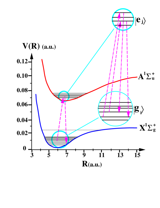
Figure 1: Schematic representation of a molecular model based on the vibrational levels in the $X^{1}\Sigma^{+}_{g}$ (lower) and $A^{1}\Sigma^{+}_{u}$ (upper) electronic surfaces of the molecule Na₂. Atomic units are chosen $\hbar=1$. $R$ denotes the internuclear distance. The arrows indicate two of the possible transitions induced by the driving field between arbitrary levels in the lower and upper surfaces. On the right is a magnified view of some of the energy levels involved and transitions between them.

The Hamiltonian of the system describes a ground and excited electronic potential energy surface coupled by a transition dipole operator:

$${\boldsymbol{\mathrm{\widehat{H}}}}\,=\,{\boldsymbol{\mathrm{\widehat{H}}}}_{g}\otimes|G\rangle\langle G|\,~{}+~{}{\boldsymbol{\mathrm{\widehat{H}}}}_{e}\otimes|E\rangle\langle E|-{\boldsymbol{\mathrm{\widehat{\mu}}}}\otimes(|G\rangle\langle E|+|E\rangle\langle G|)\cdot\epsilon(t)\,$$ (48)

where $|G\rangle$ and $|E\rangle$ are the ground and excited electronic states and ${\boldsymbol{\mathrm{\widehat{H}}}}_{g}$ and ${\boldsymbol{\mathrm{\widehat{H}}}}_{e}$ are the corresponding vibrational Hamiltonians. The electronic surfaces are coupled by the transition dipole operator ${\boldsymbol{\mathrm{\widehat{\mu}}}}$, controlled by the shaped field $\epsilon(t)$.

The present model is a simplification of the Na₂ Hilbert space restricting the number of vibrational levels. On the ground $X^{1}\Sigma^{+}_{g}$ electronic state the first $40$ vibrational levels selected out from the $66$ bound states are used. In the excited $A^{1}\Sigma^{+}_{u}$ state, the lowest $20$ vibrational states are used out of the $210$ bound levels. The vibrational Hamiltonians become therefore

$${\boldsymbol{\mathrm{\widehat{H}}}}_{g}=\sum_{i=1}^{40}E_{gi}|g_{i}\rangle\langle g_{i}|\,;\;\;\;\;\;\;{\boldsymbol{\mathrm{\widehat{H}}}}_{e}=\sum_{j=1}^{20}E_{ej}|e_{j}\rangle\langle e_{j}|\,.$$ (49)

For Na₂ the $00$ transition frequency between the ground vibrational levels of each surface is $\Omega\equiv E_{e1}-E_{g1}\approx 0.06601a.u.$ ($\sim 1.8eV$ ). A transition dipole operator independent of the internuclear distance $R$ was considered, ${\boldsymbol{\mathrm{\widehat{\mu}}}}=\mu_{0}(|G\rangle\langle E|+|E\rangle\langle G|)$. This model is sufficient for the illustrative purpose of demonstrating the execution of an algorithm in a molecular setting.

The $N=2^{Q}$ first levels of the ground electronic surface are chosen as the registers representing the $Q$ qubits. The unitary transformation implemented is a Fourier transform WPFLC01 invoked on the $N$ levels on the $X^{1}\Sigma^{+}_{g}$ electronic state representing the qubit(s). The unitary transformation is implemented through transitions between the two electronic manifolds Cf. Fig. 1.

An implementation of the iterative algorithm is chosen where the $|g_{i}\rangle\otimes|G\rangle$ and $|e_{j}\rangle\otimes|E\rangle$ eigenstates are used as the basis $\{|m\rangle\}$. The $N=2^{Q}$ first states in the lower surface are used as the basis $\{|n\rangle\}$ of the relevant subspace. The first $N-1$ energy levels plus the linear combination $\sum_{n=1}^{N}|n\rangle/\sqrt{N}$ are used as the set $|l\rangle$ for the state to state formulation. The wavefunction propagations were carried out by using a Newton polynomial integrator Kosloff94 . The final time for the implementation is $T=4.5\times 10^{4}a.u.$ ($\approx$ 1 $psec$). In all the cases a Gaussian shape function $s(t)=\exp\{-32(t/T-1/2)\}$ and a guess field $\epsilon_{guess}(t)=\epsilon_{0}s(t)\cos(\Omega t)$ were chosen.

Figure 2: Normalized functional, $J_{norm}$ versus the number of iteration: $F_{re}$ (squares), $F_{sm}$ (circles), $F_{ss}$ (triangles up) for implementing a FFT in $4$ levels. The line with triangles pointing down corresponds to $F_{ss}$ functional when $\{|l\rangle\}$ is chosen as the orthogonal basis $\{|n\rangle\}$. The objective is reached when $J_{norm}=-1.$ $\lambda_{0}=10^{3}$ and $\epsilon_{0}=5\times 10^{-3}a.u.$ in all the cases.

The implementation of the Fourier transform in $2$ qubits ($N=4$) embedded in the set of 60 levels is used for comparing the performance of the methods. Fig. 2 shows the change in the normalized functional, defined as $J_{norm}\equiv J/N$ for $F_{re}$ and $F_{ss}$, and $J_{norm}\equiv J/N^{2}$ for $F_{sm}$, with the progression of the iterative algorithm. In all the cases the target value of the normalized functional is $-1$. A large reduction in the value of the functionals is accomplished in a small number of iterations. Notice the behavior of the simultaneous state to state formulation $F_{ss}$ with an insufficient choice of the states $|l\rangle$. The algorithm finds a minimum of the objective, but, as shown in Fig. 4, the fidelity saturate at a very low value meaning that this field does not generate the target unitary transformation.

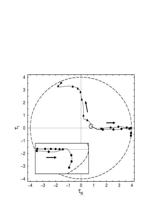
Figure 3: Evolution of the optimization in the complex $\tau$ plane for the case in Fig. 2. The lines correspond to $F_{sm}$ (circles), $F_{re}$ (squares), and $F_{ss}$ (triangles up). The open circle indicates the value of $\tau$ for the common guess field. The dashed black line is the circle $|\tau|=N$ indicating the target of the methods. The arrows mark the direction of convergence. The insert enlarges the region corresponding to the real axes close to the circumference.

Fig. 3 shows the value of $\tau$ for the field obtained in each iteration. The same initial guess was used in all the cases which constituted the starting point for all the iterative optimizations. However, the final results depend on the particular functional used. As discussed before the method based on $F_{re}$ finds a solution with a phase factor $\exp{(-i\phi)}\approx+1$.

Figure 4: Fidelity of the implementation of the 2 qubit Fourier transform versus the number of iterations $N_{it}$ for the optimization in Fig. 2. The lines correspond to $F_{re}$ (squares), $F_{sm}$ (circles), and $F_{ss}$ (triangles up). $F_{pop}$ (triangles down) denotes the case when the set $\{|l\rangle\}$ is chosen as the orthogonal basis $\{|n\rangle\}$ for the functional $F_{ss}$.

For the purpose of quantum computing the target unitary transformation has to achieve high accuracy. The fidelity functional

$${\rm fidelity}\,=\,{\rm log}_{10}(1-|\tau|^{2}/N^{2})\,.$$ (50)

is used to indicate the quality of the solution. Fig. 4 shows the improvement of the fidelity versus the iteration. The square modulus functional $F_{sm}$ Eq. (6) shows a faster convergence rate than the other two functionals.

Figure 5: Fourier transform of the optimal field result of the optimization in Fig. 4 for the functionals $F_{re}$, $F_{sm}$, and $F_{ss}$.

In Fig. 5 the Fourier transform of the field for each of the optimization procedures is shown. The large peak at the frequency $\Omega$, seen in all cases, is the result of the choice of the guess field. Besides a similar width in frequencies is found. However, the fidelity reached by the solution corresponding to the square modulus functional $F_{sm}$ is significantly better than in the other cases for the same number of iterations.

Figure 6: Fidelity versus the number of iterations for implementing a Fourier transform in $2$ (dashed-dotted line), $4$ (circles), $8$ (solid line), $16$ (dashed line) and $32$ (dotted line) levels.

The molecular model is also used to compare the convergence of the unitary transformation with the size $N$ of the relevant subspace. Fig 6 shows the improvement in the fidelity versus the number of iterations for implementing a Fourier transform in $2$, $4$, $8$, $16$, and $32$ levels ($1$, $2$, $3$, $4$, and $5$ qubits respectively). The convergence characteristics in the initial iterations strongly depends on the initial guess and the parameter $\lambda_{0}$. For example the initial guess seems inappropriate for the $1$ qubit case which displays an initial very slow convergence until after 25 iterations it find the right track. After a large number of iterations the convergence characteristics settled meaning that each new iteration was only a slight improvement on the previous one. As the iteration proceeds the rate of convergence decreases in all cases, scaling approximately as the inverse of the number of iterations. Comparing the rate of convergence for the different number of qubits after a large number of iterations the rate seems to be inversely proportional to the number of levels. High fidelity was obtained for $1$, $2$, $3$ qubit cases by continuing to $600$ iterations. The results allow to compare the integrated intensity of the optimal field:

$${\cal I}~{}=~{}\int_{0}^{T}|\mu_{0}\epsilon(t)|dt$$ (51)

The initial integrated intensity for all cases was identical. The optimization procedure changed ${\cal I}$ depending on the number of qubits. The converged results show a moderate increase of ${\cal I}$ with the number of levels starting from ${\cal I}=42$ for $1$ qubit to ${\cal I}=54$ for $2$ qubits and ${\cal I}=78$ for $3$ qubits.

V Discussion

An implicit assumption in the optimization procedure is that the system is controllable. This means that a field $\epsilon(t)$ exists which implements the unitary transformation up to a pre-specified tolerance. The problem of controllability has been the subject of several studies tarn ; Ramakrishna95 ; Ramakrishna00 ; TR01 ; schirmer02 . In the context of unitary transformations it has been shown Ramakrishna95 that if the commutators of the operators ${\boldsymbol{\mathrm{\widehat{H}}}}_{0}$ and ${\boldsymbol{\mathrm{\widehat{\mu}}}}$ generate the complete Lie group $SU(N)$, the system is completely controllable. In more concrete terms addressing the Na₂ model, it is expected to be completely controllable. The reason is that the energy levels are non degenerate and in addition each transition is distinct, characterized by a different Frank Condon factor $\langle e_{j}|{\boldsymbol{\mathrm{\widehat{\mu}}}}|g_{i}\rangle$. This controllability property will be true in almost any non-symmetric molecular system.

A far reaching conclusion is therefore that for any unitary transformation contained in the Hilbert space of the molecule, there is a driving field that implements the transformation in one step. In a molecular system this task could be achieved in a time scale of a picosecond. Since a field that executes such a unitary transformation exists, how difficult is it to find it? Does this optimal field have reasonable intensity and bandwidth?

The OCT scheme can be considered as a classical algorithm employed for the inverse problem of finding the field that generates a predefined unitary transformation. The difficulty of the inversion process is related to the scaling properties of the numerical effort with respect to the number of levels $N$. The best OCT algorithm based on the $F_{sm}$ functional is then used for estimating the scaling.

Simulating the quantum evolution is the major numerical task of the algorithm implementing OCT. The basic step is a single vector matrix multiplication which represents the operation of the Hamiltonian on the wave function. This task scales as ${\cal O}(M^{2})$ for direct vector-matrix multiplication or ${\cal O}(M\log M)$ for grid methods based on FFT k56 . The time propagation requires $N_{t}$ steps which scale as ${\cal O}(T\Delta E)$, where $\Delta E$ is the energy range of the problem.

The simulation of a unitary transformation in the relevant subspace turns out to be $N$ times more costly. Summarizing, the numerical cost of the classical simulation of the quantum propagation scales as $Cost\sim{\cal O}(2^{Q}M^{2}T\Delta E)$. This scaling relations is consistent with the fact that a classical simulation of a quantum unitary transformation scales exponentially with the number of qubits.

The numerical cost of the OCT iterative algorithm used for inversion can now be examined. The crucial question is how many iterations are required to obtain the field that implements the unitary transformation up to a specified fidelity $f$. The analysis of the results of Sec. IV show that only the initial iterative steps are very sensitive to the choice of the initial guess field. Eventually the rate of convergence reaches an asymptotic behavior where the fidelity becomes inversely proportional to the number of the iterations steps. In addition Cf. Fig. 6, the rate of convergence is also inversely proportional to the number of levels. This relation implies that the number of iterations $N_{it}$ required to achieve the fidelity $f$ becomes

$$N_{it}\approx be^{\frac{2^{Q}|f|}{a}}\,,$$ (52)

where the coefficients $a$ and $b$ are positives. The data confirm that the coefficient $a$ is independent of the number of levels $N$. The consequence of Eq. (52) is that the numerical resources required on a classical computer in order to implement the proposed scheme, scale exponentially with the number of levels $N$. Finding the field that implements in a single step a large unitary transformation is therefore prohibitively expensive. Thus fields that achieve high fidelity are only feasible for unitary transformations with a small relevant subspace. The limiting case would be the one dimensional state-to-state optimization.

Quantum control is based on interferences between many distinct pathways RZ00 . State to state coherent control finds a constructive interference which leads exclusively to the final state. The controllability depends on having a sufficient amount of interference pathways. Implementing a unitary transformation by interferences is more complex. In this case the interference pathways from one state to another have to avoid other interference paths which connect other states. The possible number of interference pathways becomes the crucial resource that allows to generate the transformation.

For weak fields, the number of pathways connecting two states in the subspace is linearly related to the number of auxiliary states on the excited surface. Practically the bandwidth of the pulse determines this number. This means that the bandwidth in a weak field implementation of a unitary transformations has to increase exponentially when the number of levels $N$ increases. The picture is completely altered when the intensity is allowed to increase. Rabi cycling increases the number of interference pathways exponentially. The number of Rabi cycles can be estimated from the integrated intensity $J_{Rabi}\sim{\cal I}/2\pi$ Cf. Eq. (51), which leads to an estimation of the number of interference pathways ${\cal O}(M^{J_{Rabi}})\sim{\cal O}(M^{{\cal I}/2\pi})$. This estimation is consistent with the results of Sec. IV where only a moderate increase in ${\cal I}$ was observed when the number of qubits in the transformation increased. The estimated number of Rabi cycles changed from $J_{Rabi}\sim 6$ for $Q=1$ to $J_{Rabi}\sim 8$ for $Q=2$ to $J_{Rabi}\sim 12$ for $Q=3$. This means that the increase in resources of implementing a unitary transformation with Q qubits in a molecular environment will scale with a low power of $T\Delta E$ where $\Delta E$ is the pulse energy.

In summary,

• A unified approach for obtaining the field that implements a unitary transformation has enabled the assessment of various formulations. In addition, a new algorithm based on the square modulus of $\tau$ was developed. This scheme was found to have superior convergence properties with respect to the number of iterations.

• A unitary transformation could be implemented in a molecular environment in a time scale of picosecond with reasonable bandwidth and intensity. For intense filed conditions the physical resources scale moderately with the number of qubits in the transformation.

• The inversion problem of finding the field that induces a unitary transformation seem to be a hard numerical problem scaling unfavorably with the number of levels in the transformation.

Appendix A The variational method

An alternative to the Krotov method of optimization is the variational method PDR88 ; RZ00 . This method has been used previously in the simultaneous $N$ state-to-state transitions formulation TV02 and for the evolution operator formulation using the functional $F_{re}$ PK02 . In the last case the variational method was generalized in terms of the evolution equation for the unitary transformation. Unlike the Krotov method the variational method does not offer a direct algorithm to minimize $F_{sm}$. For simplicity only the optimization of the functional $F_{ss}$ is discussed. The variational method is based on the functional TV02

$$K(\{\psi_{il},\psi_{fl}\},\Delta\epsilon)=\sum_{l=1}^{N}\,|\langle\psi_{il}(T)|\,{\boldsymbol{\mathrm{\widehat{O}}}}\,|l\rangle|^{2}\,-\,\int_{0}^{T}\frac{\lambda_{0}}{s(t)}\,|\Delta\epsilon|^{2}\,dt$$

$$-2\,{\rm Re}\left[\sum_{l=1}^{N}\,\langle\psi_{il}(T)|\,{\boldsymbol{\mathrm{\widehat{O}}}}\,|l\rangle\int_{0}^{T}\langle\psi_{fl}(t)|\left(\frac{d}{dt}+\frac{i}{\hbar}{\boldsymbol{\mathrm{\widehat{H}}}}(\tilde{\epsilon}+\Delta\epsilon)\right)|\psi_{il}(t)\rangle\right]\,,$$ (53)

with the additional condition $|\psi_{il}(t=0)\rangle=|l\rangle$. The set of states $\{|l\rangle\}$ and the target unitary transformation ${\boldsymbol{\mathrm{\widehat{O}}}}$ were introduced in section II. $\{|\psi_{il}(t)\}$ denotes the initial states driven by the field to the final states ${\boldsymbol{\mathrm{\widehat{O}}}}|l\rangle$. The terms $|\varphi_{fl}(t)\rangle$ are interpreted as Lagrange multipliers used as a constraint to impose the Schrödinger equation. The two first terms are equivalent to the functional (14) of the Krotov method. The parameter $\lambda_{0}$ is now interpreted as a Lagrange multiplier. The functional (A) differs from the common formulation of OCT in the form of the field term $\tilde{\epsilon}+\Delta\epsilon$. $\tilde{\epsilon}$ is a reference field and $\Delta\epsilon$ must be interpreted as the correction used to converge to the optimal field that implements the target unitary transformation. Setting $\tilde{\epsilon}=0$ and interpreting $\Delta\epsilon$ as the field the common form is re-attained.

By applying the calculus of variations, requiring $\delta K=0$, with respect to each element of the set $\{\psi_{il}(t)\}$, the evolution equations are reconstructed

$$\frac{d}{dt}|\psi_{il}(t)\rangle\,=\,-\frac{i}{\hbar}{\boldsymbol{\mathrm{\widehat{H}}}}(\tilde{\epsilon}+\Delta\epsilon)|\psi_{il}(t)\rangle\,,$$ (54)

with the condition $|\psi_{il}(t=0)\rangle=|l\rangle$ and formal solution $|\psi_{il}(t)\rangle={\boldsymbol{\mathrm{\widehat{U}}}}(t,0;\tilde{\epsilon}+\Delta\epsilon)|l\rangle$. The variations with respect to the set $\{\psi_{fl}(t)\}$ gives

$$\frac{d}{dt}|\psi_{fl}(t)\rangle\,=\,-\frac{i}{\hbar}{\boldsymbol{\mathrm{\widehat{H}}}}(\tilde{\epsilon}+\Delta\epsilon)|\psi_{fl}(t)\rangle\,,$$ (55)

with the condition $|\psi_{fl}(t=T)\rangle={\boldsymbol{\mathrm{\widehat{O}}}}|l\rangle$. The formal solution is $|\psi_{fl}(t)\rangle={\boldsymbol{\mathrm{\widehat{U}}}}(t,T;\tilde{\epsilon}+\Delta\epsilon){\boldsymbol{\mathrm{\widehat{O}}}}|l\rangle$. Finally, variations with respect to $\Delta\epsilon$ lead to the correction to the field

$$\Delta\epsilon(t)\,=\,-\frac{s(t)}{\lambda_{0}\,\hbar}{\rm Im}\left[\sum_{l=1}^{N}\,b_{l}\,\langle l|{\boldsymbol{\mathrm{\widehat{O}}}}^{\dagger}{\boldsymbol{\mathrm{\widehat{U}}}}^{\dagger}(t,T;\tilde{\epsilon}+\Delta\epsilon)\,{\boldsymbol{\mathrm{\widehat{\mu}}}}\,{\boldsymbol{\mathrm{\widehat{U}}}}(t,0;\tilde{\epsilon}+\Delta\epsilon)|l\rangle\right]\,,$$ (56)

with

$$b_{l}\,=\,\langle l|{\boldsymbol{\mathrm{\widehat{U}}}}^{\dagger}(T,0;\tilde{\epsilon}+\Delta\epsilon){\boldsymbol{\mathrm{\widehat{O}}}}|l\rangle\,.$$ (57)

The correction to the field (56) is the starting point of the iterative algorithms to find the optimal field. In such a case the correction to the field is implicit in the backwards and forwards propagation of the states in $\Delta\epsilon$. Several iterative methods have been proposed ZBR98 . In the simplest approach, a guess field $\epsilon^{(0)}$ is used to evaluate $\Delta\epsilon$, that will be used to obtain the input field in the next iteration. Usually it does not converge. An alternative procedure ZBR98 is to evaluate ${\boldsymbol{\mathrm{\widehat{U}}}}^{\dagger}$ in Eq. (56) using the field in the previous iteration and then to simultaneously obtain the correction to the field and evaluate ${\boldsymbol{\mathrm{\widehat{U}}}}$ with the new field. This iterative algorithm is identical to the one obtained from the Krotov method in Sec. III. A study comparing different iterative algorithms based on the Krotov and variational methods for the problem of state-to-state optimization is described in Ref. MT03 .

References

- (1) S. A. Rice and M. Zhao, “Optimal Control of Molecular Dynamics”, (John Wiley & Sons, Inc., New York, 2000).
- (2) M Shapiro and P. Brumer, “Principles of the Quantum Control of Molecular Processes”, (John Wiley & Sons, Inc., New Jersey, 2003).
- (3) M. A. Nielsen and I. L. Chuang, “Quantum computation and quantum information”, (Cambridge University Press, 2000).
- (4) S. Lloyd, Phys. Rev. Lett. 75, 346 (1995).
- (5) S. G. Schirmer, A. D. Greentree, V. Ramakishna, and H. Rabitz, J. Phys. A: Math. Gen. 35, 8315 (2002).
- (6) L. Tian and S. Lloyd, Phys. Rev. A 62, 050301 (2000).
- (7) R. Zadoyan, D. Kohen, D. A. Lidar, and V. A. Apkarian, Chem. Phys. 266, 323 (2001).
- (8) Z. Amitay, R. Kosloff, and S. R. Leone, Chem. Phys. Lett. 359, 8 (2002); J. Vala, Z. Amitay, B. Zhang, S. R. Leone, and R. Kosloff, Phys. Rev. A 66, 062316 (2002).
- (9) C. M. Tesch, L. Kurtz, and R. de Vivie-Riedle, Chem. Phys. Lett. 343, 633 (2001).
- (10) C. Rangan and P. H. Bucksbaum, Phys. Rev. A 64, 033417 (2001).
- (11) J. P. Palao and R. Kosloff, Phys. Rev. Lett. 89, 188301 (2002).
- (12) C. M. Tesch and R. de Vivie-Riedle, Phys. Rev. Lett. 89, 157901 (2002).
- (13) D. J. Tannor, V. Kazakov, and V. Orlov, Time Dependent Quantum Molecular Dynamics, NATO ASI Series B, Plenum, New York, 1992.
- (14) A. M. Weiner, Rev. Sci. Instrum. 71, 1929 (2000).
- (15) T. Brixner and G. Gerber, Op. Lett. 26, 557 (2001).
- (16) A. Bartana, R. Kosloff, and D. J. Tannor, Chem. Phys. 267, 195 (2001).
- (17) Y. Ohtsuki, J. Chem. Phys. 119, 661 (2003).
- (18) A. Bartana, R. Kosloff, and D. J. Tannor, J. Chem. Phys. 99, 196 (1993).
- (19) M. Sugawara, J. Chem. Phys. 118, 6784 (2003).
- (20) R. Kosloff, S. A. Rice, P. Gaspard, S. Tersigni, and D. J. Tannor, Chem. Phys. 139, 201 (1989).
- (21) A. P. Peirce, M. A. Dahleh, and H. Rabitz, Phys. Rev. A 37, 4950 (1988).
- (22) W. Zhu, J. Botina, and H. Rabitz, J. Chem. Phys. 108, 1953 (1998).
- (23) S. E. Sklarz and D. J. Tannor, Phys. Rev. A 66, 053619 (2002).
- (24) K. Sundermann and R. de Vivie-Riedle, J. Chem. Phys. 110, 1896 (1999).
- (25) T. Hornung, M. Motzkus, and R. de Vivie-Riedle, Phys. Rev. A 65, 021403 (2002).
- (26) Y. Maday and G. Turinici, J. Chem. Phys. 118, 8191 (2003).
- (27) Y. S. Weinstein, M. A. Pravia, E. M. Fortunato, S. Lloyd, and D. G. Cory, Phys. Rev. Lett. 86, 1889 (2001).
- (28) R. Kosloff, Annu. Rev. Phys. Chem. 45, 145 (1994).
- (29) V. Ramakrishna, K. Flores, H. Rabitz, R. J. Ober, Phys. Rev. A 62, 053409 (2000).
- (30) V. Ramakrishna, M. V. Salapaka, M. Dahleh , H. Rabitz, A. Peirce, Phys. Rev. A 51, 960 (1995).
- (31) G. Turinici, H. Rabitz, Chem. Phys. 267, 1 (1995).
- (32) S. G. Shirmer A. I. solomon and J. V. Leahy, J. Phys. A 35, 8551 (2002).
- (33) G. M. Huang, T. J. Tarn and J. W. Clark, J. Math. Phys. 24 2608, (1983).
- (34) Ronnie Kosloff, J. Phys. Chem., 92, 2087, (1988).