Implementing Shor’s algorithm on Josephson Charge Qubits

Abstract

We investigate the physical implementation of Shor’s factorization algorithm on a Josephson charge qubit register. While we pursue a universal method to factor a composite integer of any size, the scheme is demonstrated for the number 21. We consider both the physical and algorithmic requirements for an optimal implementation when only a small number of qubits is available. These aspects of quantum computation are usually the topics of separate research communities; we present a unifying discussion of both of these fundamental features bridging Shor’s algorithm to its physical realization using Josephson junction qubits. In order to meet the stringent requirements set by a short decoherence time, we accelerate the algorithm by decomposing the quantum circuit into tailored two- and three-qubit gates and we find their physical realizations through numerical optimization.

I Introduction

Quantum computers have potentially superior computing power over their classical counterparts Galindo ; Nielsen . The novel computing principles which are based on the quantum-mechanical superposition of states and their entanglement manifest, for example, in Shor’s integer-factorization algorithm Shor and in Grover’s database search Grover . In this paper we focus on Shor’s algorithm which is important owing to its potential applications in (de)cryptography. Many widely applied methods of public-key cryptography are currently based on the RSA algorithm Crypto which relies on the computational difficulty of factoring large integers.

Recently, remarkable progress towards the experimental realization of a quantum computer has been accomplished, for instance, using nuclear spins Steffen ; Vandersypen , trapped ions Leibfried ; Schmidt-Kaler , cavity quantum electrodynamics Yang , electrons in quantum dots Wiel , and superconducting circuits pc ; Yu ; Pashkin ; nakamura ; martinis ; vion . However, the construction of a large multiqubit register remains extremely challenging. The very many degrees of freedom of the environment tend to become entangled with those of the qubit register which results in undesirable decoherence zurek . This imposes a limit on the coherent execution time available for the quantum computation. The shortness of the decoherence time may present fundamental difficulties in scaling the quantum register up to large sizes, which is the basic requirement for the realization of nontrivial quantum algorithms DiVincenzo .

In this paper, we consider an inductively coupled charge-qubit model schon . Josephson-junction circuits provide two-state pseudospin systems whose different spin components correspond to distinct macroscopic variables: either the charges on the superconducting islands or the phase differences over the Josephson junctions. Thus, depending on the parameter values for the setup, one has flux pc ; Yu , or charge qubits Pashkin ; nakamura ; vion ; martinis ; Averin . Thus far the largest quantum register, comprising of seven qubits, has been demonstrated for nuclear magnetic resonance (NMR) in a liquid solution Vandersypen . However, the NMR technique is not believed to be scalable to much larger registers. In contrast, the superconducting Josephson-junction circuits are supposed to provide scalable registers and hence to be better applicable for large quantum algorithms You . Furthermore, they allow integration of the control and measurement electronics. On the other hand, the strong coupling to the environment through the electrical leads Storcz causes short decoherence times.

In addition to the quantum register, one needs a quantum gate “library”, i.e., a collection of control parameter sequences which implements the gate operations on the quantum register. The quantum gate library must consist of at least a set of universal elementary gates elementary , which are typically chosen to be the one-qubit unitary rotations and the CNOT gate. Some complicated gates may also be included in the library.

The quantum circuit made of these gates resembles the operational principle of a conventional digital computer. To minimize the number of gates, the structure of the quantum circuit can be optimized using methods similar to those in digital computing Aho . Minimizing the number of gates is important not only for fighting decoherence but also for decreasing accumulative errors of classical origin. If some tailored two-, three- or arbitrary $k$-qubit gates are included in the gate library, the quantum circuits may be made much more compact. The implementation of gates acting on more than two qubits calls for numerical optimization PRL . For further discussion on the implementation of non-standard gates as the building blocks for quantum circuits, see Refs. Burkard ; Schuch ; Zhang ; IJQI .

We propose an implementation of Shor’s algorithm for factoring moderately large integers - we deal with both algorithmic and hardware issues in this paper. These are two key aspects of quantum computation which, however, have traditionally been topics of disjoint research communities. Hence we aim to provide a unifying discussion where an expert on quantum algorithms can gain insight into the realizations using Josephson junctions and experimentalists working with Josephson devices can choose to read about the quantum algorithmic aspects. The background material on the construction of a quantum circuit needed for the evaluation of the modular exponential function Beauregard ; Draper is presented in Appendix A and a derivation of the effective Hamiltonian for a collection of inductively coupled Josephson qubits is given in Appendix B.

This paper is organized as follows: The construction of a quantum gate array for Shor’s algorithm is discussed in Sec. II. In Sec. III, we consider the Josephson charge-qubit register. Section IV presents the numerical methods we have employed to find the physical implementations of the gates. Section V discusses in detail how one would realize Shor’s algorithm using Josephson charge qubits to factor the number 21. Section VI is devoted to discussion.

II Shor’s factorization algorithm

With the help of a quantum computer, one could factor large composite numbers in polynomial time using Shor’s algorithm Shor ; Ekert ; Gruska ; Hirvensalo . In contrast, no classical polynomial time factorization algorithm is known to date, although the potential existence of such an algorithm has not been ruled out, either.

II.1 Quantum circuit

The strategy for the factoring of a number $N=pq$, both $p$ and $q$ being primes, using a quantum computer relies on finding the period $r$ of the modular exponential function $f(x)=a^{x}\pmod{N}$, where $0<a<N$ is a random number coprime to $N$. For an even $r$, at least one prime factor of $N$ is given by $\gcd(a^{r/2}\pm 1,N)$. Otherwise, a quantum algorithm must be executed for different values for $a$ until an even $r$ is found.

Figure 1: Quantum circuit for Shor’s algorithm.

The evaluation of $f(x)$ can be implemented using several different techniques. To obtain the implementation which involves the minimal number of qubits, one assumes that the numbers $a$ and $N$ are hardwired in the quantum circuit. However, if a large number of qubits is available, the design can be easily modified to take as an input the numerical values of the numbers $a$ and $N$ residing in separate quantum registers. The hardwired approach combined with as much classical computing as possible is considerably more efficient from the experimental point of view.

Figure 1 represents the quantum circuit  needed for finding the period $r$. Shor’s algorithm has five stages: (1) Initialization of the quantum registers. The number $N$ takes $n=\lceil\log_{2}(N+1)\rceil$ bits to store into memory, where $\lceil v\rceil$ stands for the nearest integer equal to or greater than the real number $v$. To extract the period of $f(x)$, we need at least two registers: $2n$ qubits for the register $|x\rangle_{2n}$ to store numbers $x$ and $n$ qubits for the register $|y\rangle_{n}$ to store the values of $f(x)$. The register $|x\rangle_{2n}$ is initialized as $|0\rangle_{2n}$, whereas $|y\rangle_{n}=|1\rangle_{n}$. (2) The elegance of a quantum computer arises from the possibility to utilize arbitrary superpositions. The superposition state of all integers $0\leq x\leq 2^{2n}-1$ in the register $|x\rangle_{2n}$ is generated by applying the Hadamard gate $H$ on each qubit separately. (3) The execution of the algorithm, the unitary operator $U_{f}$, entangles each input value $x$ with the corresponding value of $f(x)$:

$$U_{f}\sum_{x}|x\rangle|1\rangle=\sum_{x}|x\rangle|a^{x}\!\!\!\pmod{N}\rangle.$$ (1)

(4) The quantum Fourier transformation (QFT) is applied to the register $|x\rangle_{2n}$, which squeezes the probability amplitudes into peaks due to the periodicity $f(x)=f(x+r)$. (5) A measurement of the register $|x\rangle_{2n}$ finally yields an indication of the period $r$. A repetitive execution of the algorithm reveals the probability distribution which is peaked at the value $2^{2n}$/$r$ and its integer multiples of output values in the register $|x\rangle_{2n}$.

Besides the quantum algorithm which is used to find $r$, a considerable amount of classical precomputing and postprocessing is required as well. However, all this computing can be performed in polynomial time.

II.2 Implementing the modular exponential function

We are looking for a general scalable algorithm to implement the required modular exponential function. The implementation of this part of the algorithm sets limits for the spatial and temporal requirements of computational resources, hence it requires a detailed analysis. The remarkable experimental results Vandersypen to factor the number 15 involve an elegant quantum circuit of seven qubits and only a few simple quantum gates. The implementation definitely exploits the special properties of the number 15, and the fact that the outcome of the function $a^{x}\pmod{N}$ can be calculated classically in advance for all input values $x$ when $N$ is small. For arbitrary $N$, reversible arithmetic algorithms must be employed Beckman ; Vedral . The classical arithmetic algorithms Knuth , can be implemented reversibly by replacing the irreversible logic gates by their reversible counterparts. The longhand multiplication algorithm, which we use below, should be optimal up to very large numbers, requiring only $O(n)$ qubits and $O(n^{3})$ step.

The implementation of the modular exponential function using a longhand multiplication algorithm and a QFT-based adder Beauregard provides us with small scratch space requiring only a total space of $4n+2$ qubits. The details of the implementation are given in Appendix A. The conventional approach to longhand multiplication without a QFT-based adder would require on the order of $5n$ qubits. The price of the reduced space is the increase in the execution time, which now is $O(n^{4})$, but which can be reduced down to $O(n^{3}\log_{2}\frac{n}{\epsilon})$, allowing for a certain error level $\epsilon$. According to Ref. Beauregard one would achieve an algorithm requiring only $2n+3$ qubits with intermediate measurements. However, we do not utilize this implementation since the measurements are likely to introduce decoherence.

III Josephson charge-qubit register

The physical model studied in this paper is the so-called inductively coupled Cooper pair box array. This model, as well as other related realizations of quantum computing, has been analyzed in Ref. schon . The derivation of the Hamiltonian is outlined in Appendix B for completeness. Our approach to quantum gate construction is slightly different from those found in the literature and it is therefore worthwhile to consider the physical model in some detail.

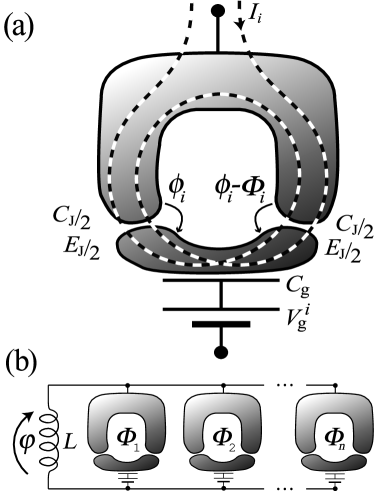
Figure 2: a) Schematic of a Josephson charge qubit with the relevant parameters. b) An array of Josephson charge qubits coupled in parallel with an inductor.

A schematic picture of a homogeneous array of qubits is shown in Fig. 2. Each qubit $i$ comprises a superconducting island coupled capacitively to a gate voltage and a SQUID loop through which Cooper pairs may tunnel. The gate voltage may be used to tune the effective gate charge $n_{\rm g}^{i}$ of the island whereas the external magnetic flux through the SQUID can be used to control the effective Josephson energy. Each qubit is characterized by a charging energy $E_{\rm C}$ and a tunable Josephson energy $E_{\rm J}(\Phi_{i})$, where $\Phi_{i}$ is the flux threading the SQUID. The Hamiltonian for the $i^{\rm th}$ qubit can be written as

$${\cal H}^{i}_{\text{single}}=-\frac{1}{2}B^{i}_{z}\sigma_{z}^{i}-\frac{1}{2}B^{i}_{x}\sigma_{x}^{i}$$ (2)

and the coupling between the $i^{\rm th}$ and $j^{\rm th}$ qubits as

$${\cal H}_{\text{coupling}}^{i,j}=-CB^{i}_{x}B^{j}_{x}\sigma_{y}^{i}\otimes\sigma_{y}^{j}\,\,.$$ (3)

The qubit state $|0\rangle$ (“spin up”) corresponds to zero extra Cooper pairs residing on the island and the state $|1\rangle$ (“spin down”) corresponds to one extra pair on the island. Above $B^{i}_{x}=E_{\rm J}(\Phi_{i})$, $B^{i}_{z}=E_{\rm C}(1-2n_{\rm g}^{i})$ and $C=\pi^{2}L/\Phi_{0}^{2}\left(C_{\rm qb}/C_{\rm J}\right)^{2}$ denotes the strength of the coupling between the qubits, whereas $C_{\rm qb}$ is the total capacitance of a qubit in the circuit, $C_{\rm J}$ is the capacitance of the SQUID, $L$ is the inductance which may in practice be caused by a large Josephson junction operating in the linear regime and finally $\Phi_{0}=h/2e$ is the flux quantum. The approach taken is to deal with the parameters $B^{i}_{z}$ and $B^{i}_{x}$ as dimensionless control parameters. We assume that they can be set equal to zero which is in principle possible if the SQUID junctions are identical. We set $C=1$ and choose natural units such that $\hbar=1$.

The Hamiltonian in Eqs. (2–3) is a convenient model for studying the construction of quantum algorithms for a number of reasons. First of all, each single-qubit Hamiltonian can be set to zero, thereby eliminating all temporal evolution. Secondly, setting the effective Josephson coupling to zero eliminates the coupling between any two qubits. This is achieved by applying half a flux quantum through the SQUID loops. If the Josephson energy of any two qubits is nonzero, there will automatically emerge a coupling between them. This is partly why numerical methods are necessary for finding the control-parameter sequences. By properly tuning the gate voltages and fluxes it is possible to compensate undesired couplings and to perform any temporal evolution in this model setup.

We note that the generators $i\sigma_{x}$ and $i\sigma_{z}$ are sufficient to construct all the $SU(2)$ matrices through the Baker-Campbell-Hausdorff formula and thus single-qubit gates need not be constructed numerically. It is even possible to do this in a piecewise linear manner avoiding abrupt switching since the only relevant parameter is the time integral of either $B^{i}_{z}$ or $B^{i}_{x}$ if only one of them is nonzero at a time. That is, any $U\in SU(2)$ acting on the i^th qubit can be written as

$$U=e^{i\sigma_{z}^{i}\int_{t_{2}}^{t_{3}}B_{z}^{i}(t)dt/2}e^{i\sigma_{x}^{i}\int_{t_{1}}^{t_{2}}B_{x}^{i}(t)dt/2}e^{i\sigma_{z}^{i}\int_{t_{0}}^{t_{1}}B_{z}^{i}(t)dt/2},$$ (4)

where we assume that from $t_{0}$ to $t_{1}$ only $B^{i}_{z}$ is nonzero, from $t_{1}$ to $t_{2}$ only $B^{i}_{x}$ is nonzero and from $t_{2}$ to $t_{3}$ only $B^{i}_{z}$ is again nonzero. For instance, the gate $iH\in SU(2)$, equivalent to the Hadamard gate $H\in U(2)$ up to a global phase, can be realized as in Fig. 3 by properly choosing the time-integrals in Eq. (4). We cannot achieve $U(2^{n})$ for $n$ qubits since the Hamiltonian for the entire quantum register turns out to be traceless, thus producing only $SU(2^{n})$ matrices. However, the global phase factor is not physical here since it is not observable.

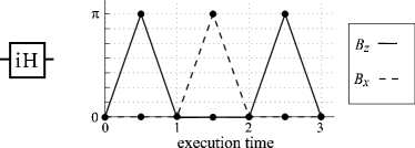
Figure 3: Pulse sequence implementing an equivalent of the Hadamard gate. Solid line indicates $B_{x}^{i}$ while the dashed line shows $B_{z}^{i}$.

The above Hamiltonian is an idealization and does not take any decoherence mechanisms into account. To justify this omission, we have to ensure that a charge-qubit register is decoherence-free for time scales long enough to execute a practical quantum algorithm. In addition, we have neglected the inhomogenity of the SQUIDs. It may be extremely challenging to fabricate sufficiently uniform junctions. A three-junction design might alleviate this problem. Whereas for the control of $N$ two-junction SQUIDs one needs at least $N$ independent sources of flux, the three-junction design would call for $2N$ independent sources. The extra sources may be used to compensate the structural nonuniformities. The noise in the control parameters has also been neglected but it will turn out that the error will grow linearly with the rms displacement of uncorrelated Gaussian noise. Correlated noise may only be tolerated if it is very weak. We have also neglected the issue of quantum measurement altogether in the above.

A crucial assumption is that $k_{\rm B}T\ln N_{\rm qp}\ll E_{\rm J}\ll E_{\rm C}\ll\Delta_{\rm BCS}$, where $N_{\rm qp}$ is the number of quasiparticle modes. Typical operation frequencies would be in the GHz range and the operation temperature could be tens of mK. For our two-state Hamiltonian to apply, we should actually insist that, instead of $E_{\rm J}\ll E_{\rm C}$, the requirement $E_{\rm J}(\Phi_{i})\ll E_{\rm C}$ holds. It may appear at first that $B_{x}^{i}$ cannot take on values exceeding $B_{z}^{i}$. However, this does not hold since the gate charge also plays a role; values of $B_{z}^{i}$ can be very small if $n_{\rm g}^{i}$ is tuned close to one half. Since we employ natural units we may freely rescale the Hamiltonian while rescaling time. This justifies our choice $C=1$ above. Furthermore, it is always possible to confine the parameter values within an experimentally accessible range. For more discussion, see Ref. schon .

IV Implementing a Quantum-gate Library

The evaluation of the time-development operator $U$ is straightforward once the externally controlled physical parameters for the quantum register are given. Here we use numerical optimization to solve the inverse problem; namely, we find the proper sequence for the control variables which produce the given quantum gate.

IV.1 Unitary time evolution

The temporal evolution of the Josephson charge-qubit register is described by a unitary operator

$$U_{\gamma(t)}=\mathcal{T}\exp\left(-i\int_{\gamma(t)}{\cal H}(\gamma(t))dt\right),$$ (5)

where $\mathcal{T}$ stands for the time-ordering operator and ${\cal H}(\gamma(t))$ is the Hamiltonian for the qubit register. The integration is performed along the path $\gamma(t)$ which describes the time evolution of the control parameters in the space spanned by $\{B_{x}^{j}(t)\}$ and $\{B_{z}^{j}(t)\}$.

Instead of considering paths $\gamma(t)$ with infinitely many degrees of freedom, we focus on paths parametrized by a finite set of parameters $X_{\gamma}$. This is accomplished by restricting the path $\gamma(t)$ to polygons in the parameter space. Since the pulse sequence starts and ends at the origin, it becomes possible to consistently arrange gates as a sequence. For an $n$-qubit register, the control-parameter path $\gamma(t)$ is of the vector form

$$\gamma(t)=\left[\begin{matrix}B_{z}^{1}(t),&\dots&,B_{z}^{n}(t);&B_{x}^{1}(t),&\dots&,B_{x}^{n}(t)\end{matrix}\right]^{T},$$ (6)

where $B_{z}^{i}(t)$ and $B_{z}^{i}(t)$ are piecewise linear functions of time for the chosen parametrization. Hence, in order to evaluate Eq. (5), one only needs to specify the $2n$ coordinates for the $\nu$ vertices of the polygon, which we denote collectively as $X_{\gamma}$. We let the parameter loop start at the origin, i.e., at the degeneracy point where no time development takes place. We further set the time spent in traversing each edge of the polygon to be unity.

In our scheme, the execution time for each quantum gate depends linearly on the number $\nu$ of the vertices in the parameter path. This yields a nontrivial relation between the execution time of the algorithm and the size of the gates. First note that each $k$-qubit gate represents a matrix in $SU(2^{k})$. To implement the gate, one needs to have enough vertices to parameterize the unitary group $SU(2^{k})$, which has $2^{2k}-1$ generators. In our model, we have $2k$ parameters for each vertex, which implies $2k\nu\geq 2^{2k}-1.$ We have used $\nu=4$ for the two-, and $\nu=11$ for the three-qubit gates.

To evaluate the unitary operator $U_{\gamma(t)}$ we must find a numerical method which is efficient, yet numerically stable. We divide the path $\gamma(t)$ into tiny intervals that take a time $\Delta t$ to traverse. If $\gamma_{i}$ collectively denotes the values of all the parameters in the midpoint of the $i^{\rm th}$ interval, and $m$ is the number of such intervals, we then find to a good approximation

$$U_{X_{\gamma}}\approx\exp(-i{\cal H}(\gamma_{m})\Delta t)\ldots\exp(-i{\cal H}(\gamma_{1})\Delta t)\,.$$ (7)

We employ the truncated Taylor series expansion

$$e^{-i{\cal H}\Delta t}\approx\sum_{k=0}^{l}\frac{(-i{\cal H}\Delta t)^{k}}{k!}$$ (8)

to evaluate each factor in Eq. (7). We could use the Cayley form

$$e^{-i{\cal H}\Delta t}\approx(1-i{\cal H}\Delta t/2)(1+i{\cal H}\Delta t/2)^{-1},$$ (9)

or an adaptive Runge-Kutta method to integrate the Schrödinger equation as well. It turns out that the Taylor expansion with $l=3$ is fast and yields enough precision for our purposes. The precision and unitarity of the approximation are verified by comparing the results with those obtained with an exact spectral decomposition of ${\cal H}$.

IV.2 Minimization of the error function

Given an arbitrary matrix $\hat{U}$, our aim is to find a parameter sequence $X_{\gamma}$ for the Josephson charge-qubit register that yields a unitary matrix $U_{X_{\gamma}}=\hat{U}$. We convert the inverse problem into an optimization task; namely, that of finding the zeroes of the error function

$$p(X_{\gamma})=\|\hat{U}-U_{X_{\gamma}}\|_{\rm F}.$$ (10)

Minimizing $p(X_{\gamma})$ over all the possible values of $X_{\gamma}$ will produce an approximation $U_{X_{\gamma}}$ for the desired gate $\hat{U}$. Above $\|\cdot\|_{\rm F}$ denotes the Frobenius trace norm, defined as $\|{A}\|_{\rm F}=\sqrt{\mathrm{Tr}\left({A}^{\dagger}{A}\right)}$, which is numerically efficient to compute. Since all the matrix norms are mathematically equivalent, a small value of $\|{A}\|_{\rm F}$ implies a small value in all other norms as well, see e.g. Ref. golub .

For this minimization problem, the error-function landscape is rough consisting of many local minima. Consequently, any gradient-based minimization algorithm will encounter serious problems. Thus, we have found the minimum point $X_{\rm min}$ for all the gates presented in Sec. V using repeated application of a robust polytope algorithm IJQI ; Reva ; poly . In the first search, the initial condition was chosen randomly. At the next stage, the outcome of the previous search was utilized. In order to accelerate the evaluation of $U_{\gamma(t)}$ we varied the time steps $\Delta t$; at an early stage of the optimization a coarse step was employed while the final results were produced using very fine steps. Typical convergence of the search algorithm is illustrated in Fig. 4.

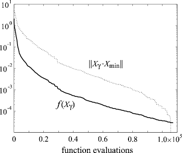
Figure 4: Convergence of the algorithm for the Fredkin gate. The error function values are indicated by the solid line and the distance of the parameter sequence from the numerical optimum $X_{\rm min}$ by the dotted line.

The required accuracy for the gate operations is in the range $10^{-4}$ – $10^{-5}$ for $p(X_{\gamma})$ for two reasons: (i) in quantum circuits with a small number of gates, the total error remains small, and (ii) for large circuits, quantum-error correction can in principle be utilized to reduce the accumulated errors DiVincenzo . Our minimization routine takes on the order of $10^{6}$ function evaluations to reach the required accuracy.

V Example

To demonstrate the level of complexity for the quantum circuit and the demands on the execution time, we explicitly present the quantum circuit and some physical implementation for the gates needed for Shor’s algorithm to factor the number $N=21$. We choose $a=11$ and hardwire this into the quantum circuit.

V.1 Quantum Circuit

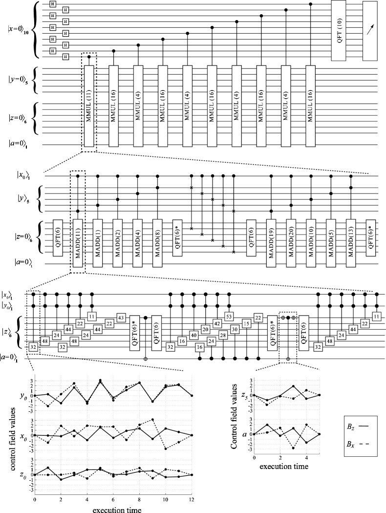
Figure 5: Quantum circuit for Shor’s algorithm factoring the number 21 with the parameter value $a=11$. The full circuit is shown topmost and the decompositions of the modular multiplier and adder blocks are indicated with dashed lines. The gates in the circuit have their conventional meanings, except that we denote a phase-shift gate by a box with a single number $\phi$ in it meaning that the phase of the state $|1\rangle$ is shifted by $e^{2\pi i\phi/2^{n}}$ with respect to the state $|0\rangle$. Two examples of numerically optimized parameter sequences are also shown.

Figure 5 illustrates the structure of the quantum part of the factorization algorithm for the number 21. Since it takes 5 bits to store the number 21, a 5-qubit register $|y\rangle_{5}$ and a 10-qubit register $|x\rangle_{10}$ are required.

For scratch space we need a six-qubit register $|z\rangle_{6}$ and one ancilla qubit $|a\rangle$. Each thirteen-qubit controlled-MMUL (modular multiplier) gate in the algorithm can be further decomposed as indicated in Fig. 5. The controlled-MADD (modular adder) gates can also be decomposed. The ten-qubit QFT breaks down to 42 two-qubit gates and one three-qubit QFT. Similarly, the six-qubit QFT can be equivalently implemented as a sequence of 18 two-qubit gates and one three-qubit QFT. In this manner we can implement the entire algorithm using only one-, two- and three-qubit gates. The control parameter sequence realizing each of them can then be found using the scheme outlined in Sec. IV. Two examples of the pulse sequences are also shown in Fig. 5 (bottom insets).

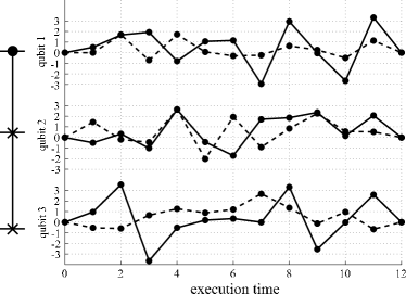
Figure 6: Control parameters for the Fredkin gate. Solid line indicates $B_{z}^{i}$ while the dashed line shows $B_{x}^{i}$.

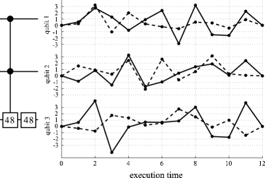
Figure 7: Control parameters for a composite gate consisting of a controlled² phase shift and a one-qubit rotation, see text. Solid line indicates $B_{z}^{i}$ while the dashed line shows $B_{x}^{i}$.

V.2 Physical implementation

The experimental feasibility of the algorithm depends on how complicated it is compared to the present state of technology. Following the above construction of the quantum circuit, the full Shor algorithm to factor 21 requires about 2300 three-qubit gates and some 5900 two-qubit gates, in total. Also a few one-qubit gates are needed but alternatively they can all be merged into the multi-qubit gates. If only two-qubit gates are available, about 16400 of them are required. If only a minimal set of elementary gates, say the CNOT gate and one-qubit rotations are available, the total number of gates is remarkably higher. In our scheme the execution time of the algorithm is proportional to the total length of the piecewise linear parameter path which governs the physical implementation of the gate operations. Each of the three-qubit gates requires at least a 12-edged polygonal path $\gamma(t)$ whereas two-qubit gates can be implemented with 5 edges. Consequently, on the order of 57100 edges are required for the whole algorithm if arbitrary three-qubit gates are available, whereas $\sim$ 82000 edges would be required for an implementation with only two-qubit gates.

The ability to find the physical implementation of the gate library for Shor’s algorithm is demonstrated with some further examples. Figure 6 shows how to physically implement the controlled swap gate. We have taken advantage of tailored three-qubit implementations: a one-qubit phase-shift gate and a three-qubit controlled² phase-shift gate are merged into one three-qubit gate, see Fig. 7.

The control parameter sequences presented will yield unitary operations which approximate the desired gate operations with an accuracy better than $10^{-4}$ in the error-function values for the three-qubit gates. For two-qubit gates the error is negligible. Since the whole factorization circuit consists of some $10^{3}$ three-qubit gates, we obtain a total error of $\sim 10^{-1}$. This is sufficient for the deduction of the essential information from the output. The robustness of the gates obtained was studied numerically by adding Gaussian noise to the vertices of the path. The error function was found to scale linearly with the rms of the variance of the Gaussian noise: error $\approx$ 6 $\times\langle{\rm noise}\rangle_{\rm rms}$, which is probably acceptable.

VI Discussion

In this paper we have discussed the implementation of Shor’s factorization algorithm using a Josephson charge-qubit register. This method is suitable for the first experimental demonstration of factoring a medium-scale integer $2^{4}$ – $2^{20}$. As an example of this method we have studied the algorithm for factoring 21. The only integer smaller than 21 for which Shor’s algorithm is applicable is 15, but this is a special case having only the periods 2 and 4. For the experimental factoring of 15 one should consider more direct methods Vandersypen to implement the modular exponential function. For a larger integer $N$ other approaches, e.g. the Schönhage-Strassen multiplication algorithm, will provide a more efficient quantum circuit. Our approach of numerically determining the optimized gates can be generalized to other physical realizations with tunable couplings as well. The only requirement is that the system allows total control over the control parameters.

We have found that the number of qubits and quantum gates that are involved in carrying out the algorithm is rather large from the point of view of current technology. Thus the realization of a general factorization algorithm for a large integer $N$ will be challenging. Consequently, the scaling of the chosen algorithm, both in time and space, will be of prime importance.

The method we propose utilizes three-qubit gates, which compress the required quantum-gate array, resulting in a shorter execution time and smaller errors. One should also consider other implementations of the quantum algorithms that employ gates acting on a larger number of qubits to further decrease the number of gates and execution time. For example, four-qubit gates may be achievable, but this involves harder numerical optimization.

Finally, let us consider the experimental feasibility of our scheme. To factor the number 21, we need on the order of $10^{4}$ edges along the control-parameter path. Assuming that the coherence time is on the order of 10^-6 s implies that the upper limit for the duration of each edge is 10^-10 s. Since our dimensionless control parameters in the examples are on the order of unity, the energy scale in angular frequencies must be at least on the order of 10¹⁰ s^-1. Typical charging energies for, say, thin-film aluminum structures may be on the order of $10^{-23}J$ which corresponds to $10^{11}$ s^-1. The ultimate limiting energy scale is the BCS gap, which for thin-film aluminum corresponds to an angular frequency of about $3\times 10^{11}$ s^-1. Based on these rough estimates, we argue that factoring the number 21 on Josephson charge qubits is, in principle, experimentally accessible.

Constructing a quantum algorithm to decrypt RSA-155 coding which involves a 512-bit integer $N$ with the scheme that we have presented would require on the order of $2000$ qubits. Assuming that the execution time scales as $n^{3}\log n$ implies that tens of seconds of decoherence time is needed. This agrees with the estimates in Ref. Hughes and poses a huge experimental challenge. This can be compared to the 8000 MIPS (Million Instructions Per Second) years of classical computing power which is needed to decrypt the code using the general numeric field sieve technique Galindo . Thus Shor’s algorithm does appear impractical for decrypting RSA-155. However, it provides the only known potentially feasible method to factor numbers having 1024 or more bits.

We conclude that it is possible to demonstrate the implementation of Shor’s algorithm on a Josephson charge-qubit register. Nevertheless, for successful experimental implementation of large-scale algorithms significant improvements in coherence times, fabrication and ultrafast control of qubits is mandatory.

Note added: After the completion of the revised version of this manuscript, it was brought to our attention that the implementation of Shor’s algorithm has recently also been considered for a linear nearest-neighbor (LNN) qubit array model Fowler . In an approach similar to ours, however, the LLN quantum-circuit model is independent of any specific physical realization.

Appendix A Construction of Quantum circuit

Here we represent the construction of a quantum circuit needed for an evaluation of the modular exponential function $a^{x}\pmod{N}$. We assume the values of $a$ and $N$ to be constant integers coprime to each other. This approach takes advantage of the well-known fast powers trick, as well as the construction of a multiplier suggested by Beauregard Beauregard , which in part employs the adder of Draper Draper .

The modular exponential function can be expressed in terms of modular products:

$$a^{x}\equiv\prod_{i=0}^{2n-1}(a^{2^{i}x_{i}}\pmod{N})\pmod{N},$$ (11)

where we have used the binary expansion $x=2^{0}x_{0}+2^{1}x_{1}+2^{n-1}x_{n-1}$, $x_{i}\in$ {0,1}. Note that the number of factors in Eq. (11) grows only linearly for increasing $n$. The longhand multiplication is based on the relation

$$a^{2^{i}}x\equiv\sum_{k=0}^{2n-1}\,(a^{2^{i}}2^{k}x_{k}\pmod{N})\!\!\!\!\pmod{N},$$ (12)

which again involves only a linear number of terms.

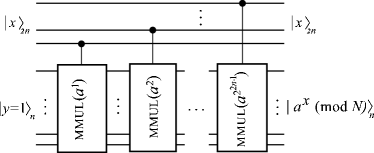
Figure 8: Quantum circuit required for performing the evaluation of the modular exponential function utilizing the CMMUL($b$) gates.

Equation (11) yields a decomposition of the modular exponential function into controlled modular multiplication gates (CMMUL($a^{2^{i}}$)), see Fig. 8. According to Eq. (12), each of the MMUL($a^{2^{i}}$) gates can be implemented with the sequence of the modular adders, see Fig. 9. Since this decomposition of CMMUL($a^{2^{i}}$) requires extra space for the intermediate results, we are forced to introduce a scratch space $|z\rangle_{n+1}$ into the setup. Initially, we set $|z\rangle_{n+1}=|0\rangle_{n+1}$. Moreover, we must reset the extra scratch space after each multiplication. Euler’s totient theorem guarantees that for every $b$ which is coprime to $N$, a modular inverse $b^{-1}\in\mathbb{N}$ exists. Furthermore, the extended Euclidean algorithm provides an efficient way to find the numerical value for $b^{-1}$.

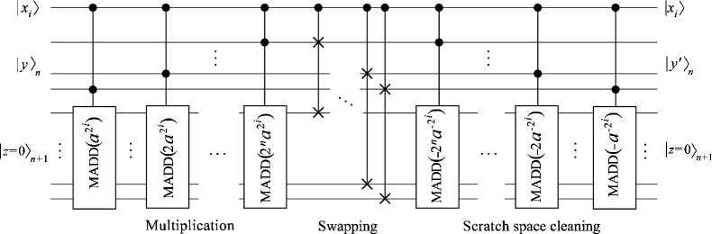
Figure 9: Decomposition of the CMMUL($a^{2^{i}}$) gate using C²MADD($b$) and controlled swap gates. If the controlling qubit $|x_{i}\rangle$ is active the resulting state is $y^{\prime}\equiv y+a^{2^{i}}\pmod{N}$, otherwise $y^{\prime}=y$. Note, that the gate utilizes an additional ancilla register $|z\rangle_{n}$ to perform the calculation.

Figure 10 presents decomposition of the C²MADD($b$) gate ($b\in\mathbb{N}$ using adders in the Fourier space. An obvious drawback of this implementation is the need for a number of QFT-gates. However, we need to introduce only one ancilla qubit $|a\rangle$. The decomposition of the gate C²MADD($b$) consists of controlled² adders, $(n+1)$-qubit QFTs, one-qubit NOTs, and CNOTs. The decomposition of a QFT-gate into one- and two-qubit gates is presented, for instance, in Ref. Nielsen . Since Fourier space is utilized, the C²ADD($b$) gates can be implemented Draper using controlled² phase shifts. The quantum gate sequence for an adder working in the Fourier space is depicted in Fig. 11. The values of the phase shifts for the gate C²ADD($b$) are given by $e^{2\pi i\phi_{j}/2^{n}}$, where $\phi_{j}=2^{j}b$.

Finally, we are in the position to perform the unitary transformation which implements the modular exponential function using only one-, two- and three-qubit gates. If the three-qubit gates are not available, further decomposition into one- and two-qubit gates is needed, see Ref. elementary . For instance, each three-qubit controlled²U gate decomposes into five two-qubit gates and each Fredkin gate takes seven two-qubit gates to implement.

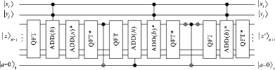
Figure 10: Decomposition of the C²MADD($b$) gate into elementary gates, QFT gates, and additions in the Fourier basis (C²ADD). The asterisk stands for a Hermitian conjugate; it corresponds to a gate for subtraction. The gate takes an input value $z<N\leq 2^{n}$ and yields $|z^{\prime}\rangle_{n+1}=|z+b\pmod{N}\rangle_{n+1}$ if the control qubits $x_{i}=1$ and $y_{j}=1$. Otherwise $|z^{\prime}\rangle_{n+1}=|z\rangle_{n+1}$. The ancilla qubit $|a\rangle$ is one if $z+b>N$ and zero otherwise.

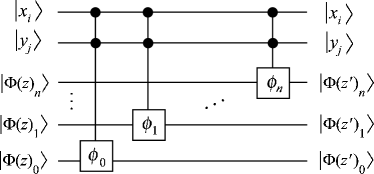
Figure 11: Quantum circuit for the controlled² addition of a classical number $b$ into the quantum register $|z\rangle_{n+1}$ in the Fourier basis. The controlled² phase-shift gates serve to yield the phase shift $e^{2\pi i\phi_{k}/2^{n}}$ provided that the control qubits $|x_{i}\rangle$ and $|y_{j}\rangle$ are active.

Appendix B Derivation of the Hamiltonian

B.1 The Lagrangian

Consider a homogenous array of mesoscopic superconducting islands as an idealized model of a quantum register, see Fig. 2. The basis states of the qubit correspond to either zero or one extra Cooper pair residing on the superconducting island, denoted by $|0\rangle$ and $|1\rangle$, respectively. Each of the islands, or Cooper-pair boxes, is capacitively coupled to a gate voltage, $V_{\rm g}^{i}$. In addition, they are coupled to a superconducting lead through a mesoscopic SQUID with identical junctions, each having the same Josephson energy $E_{\rm J}/2$ and capacitance $C_{\rm J}/2$. All these qubits are then coupled in parallel with an inductor, $L$. The lowest relevant energy scale is set by the thermal energy $k_{\rm B}T$ and the highest scale by the BCS gap $\Delta_{\rm BCS}$.

We assume that the gate voltage $V_{\rm g}^{i}$ and the time-dependent flux $\Phi_{i}$ through each SQUID can be controlled externally. The flux $\Phi_{i}$ may be controlled with an adjustable current $I_{i}$ through an external coil, see the dotted line in Fig. 2a. In this setup, the Cooper pairs can tunnel coherently to a superconducting electrode. We denote the time-integral of voltage, or difference in flux units, over the left junction of the $i^{\rm th}$ SQUID by $\phi_{i}$ and the flux through the inductor by $\varphi$. The phase difference in flux units over the rightmost junction is $\phi_{i}-\Phi_{i}$. We take the positive direction for flux to be directed outward normal to the page.

We adopt $\phi_{i}$ and $\varphi$ as the dynamical variables, whereas $\Phi_{i}$ and $V_{\rm g}^{i}$ are external adjustable parameters. With the help of elementary circuit analysis Devoret , we obtain the Lagrangian for the qubit register

$$\mathcal{L} =\frac{1}{2}\sum_{i=1}^{n}\left[\frac{C_{\rm J}}{2}\dot{\phi}_{i}^{2}+\frac{C_{\rm J}}{2}(\dot{\phi}_{i}-\dot{\Phi}_{i})^{2}+C_{\rm g}(\dot{\phi}_{i}+\dot{\varphi}-V_{\rm g}^{i})^{2}\right]$$

$$-\frac{\varphi^{2}}{2L}+\frac{1}{2}\sum_{i=1}^{n}\left[E_{\rm J}\cos\left(\frac{2e}{\hbar}\phi_{i}\right)+E_{\rm J}\cos\left(\frac{2e}{\hbar}(\phi_{i}-\Phi_{i})\right)\right].$$ (13)

We now perform the following changes of variables

$$\phi_{i}\to\phi_{i}+\frac{\Phi_{i}}{2}-\frac{C_{\rm g}}{C_{\rm J}+C_{\rm g}}\varphi$$ (14)

which yields

$$\mathcal{L} =\frac{1}{2}\sum_{i=1}^{n}\left[(C_{\rm J}+C_{\rm g})\dot{\phi}_{i}^{2}-2C_{\rm g}\left(V_{\rm g}^{i}-\frac{\dot{\Phi}_{i}}{2}\right)\dot{\phi}_{i}\right.$$

$$\left.+E_{\rm J}\cos\left(\pi\frac{\Phi_{i}}{\Phi_{0}}\right)\cos\left(\frac{2e}{\hbar}\phi_{i}-\frac{2\pi C_{\rm qb}}{\Phi_{0}C_{\rm J}}\varphi\right)\right]$$

$$+\frac{1}{2}NC_{\rm qb}\dot{\varphi}^{2}-\sum_{i=1}^{n}C_{\rm qb}(V_{\rm g}^{i}-\frac{\dot{\Phi}_{i}}{2})\dot{\varphi}-\frac{\varphi^{2}}{2L}$$ (15)

$$+{\rm const}.$$ (16)

Above, $\Phi_{0}=h/2e$ is the flux quantum and $C_{\rm qb}=C_{\rm J}C_{\rm g}/(C_{\rm J}+C_{\rm g})$ is the qubit capacitance in the $LC$-circuit. Note that the effective Josephson energy of each SQUID can now be tuned. We denote this tunable energy parameter in Eq. (16) as

$$E_{\rm J}(\Phi_{i})=E_{\rm J}\cos\left(\pi\frac{\Phi_{i}}{\Phi_{0}}\right).$$ (17)

The canonical momenta are given by $Q=\partial\mathcal{L}/\partial\dot{\varphi}$ and $q_{i}=\partial\mathcal{L}/\partial\dot{\phi}_{i}$. We interpret $Q$ as the charge on the collective capacitor formed by the whole qubit register, whereas $q_{i}$ is the charge on the $i^{\rm th}$ island. Note that the charge $q_{i}$ is related to the number $n_{i}$ of Cooper pairs on the island through $q_{i}=-2en_{i}$.

B.2 The Hamiltonian

We are now in the position to write down the Hamiltonian for the quantum register. We will also immediately replace the canonical variables by operators in order to quantize the register. Moreover, we will employ the number of excess Cooper pairs $n_{i}$ on the island and the superconducting phase difference instead of the usual quantum-mechanical conjugates. We will also change to the more common phase difference $\theta_{i}$ related to $\phi_{i}$ through $\theta_{i}=\frac{2e}{\hbar}\phi_{i}$. Hence the relevant commutation relations are $[\theta_{i},n_{i}]=-i$ and $[\varphi,Q]=i\hbar$. All the other commutators vanish. Using the Legendre transformation

$$\mathcal{H}=Q\dot{\varphi}+\sum_{i=1}^{n}q_{i}\dot{\phi}_{i}-\mathcal{L}$$ (18)

we obtain

$$\mathcal{H} =\sum_{i=1}^{n}\left[\frac{2e^{2}(n_{i}-n_{\rm g}^{i})^{2}}{C_{\rm J}+C_{\rm g}}-E_{\rm J}(\Phi_{i})\cos\left(\theta_{i}-\frac{2\pi C_{\rm qb}}{\Phi_{0}C_{\rm J}}\varphi\right)\right]$$

$$+\frac{(Q+Q_{\rm g})^{2}}{2NC_{\rm qb}}+\frac{\varphi^{2}}{2L}.$$ (19)

We have denoted the effective gate charge by

$$n_{\rm g}^{i}=\frac{C_{\rm g}}{2e}\left(V_{\rm g}^{i}-\frac{\dot{\Phi}_{i}}{2}\right)$$ (20)

and

$$Q_{\rm g}=\sum_{i=1}^{n}C_{\rm qp}\left(V_{\rm g}^{i}-\frac{\dot{\Phi}_{i}}{2}\right).$$ (21)

In addition to the usual voltage contribution, the time dependence of the flux also plays a role. In practice, the rates of change of the flux are negligible in comparison to the voltages and this term may safely be dropped.

The Hamiltonian in Eq. (B.2) describes the register of qubits ($n_{i},\phi_{i}$) coupled to a quantum-mechanical $LC$-resonator, i.e., a harmonic oscillator ($Q,\varphi$). We will now assume that the rms fluctuations of $\varphi$ are small compared to the flux quantum $\Phi_{0}$ and also that the harmonic oscillator has a sufficiently high frequency, such that it stays in the ground state. The first assumption implies that

$$\cos\left(\theta_{i}-\frac{2\pi C_{\rm qb}}{\Phi_{0}C_{\rm J}}\varphi\right)\approx\cos\theta_{i}+\frac{2\pi C_{\rm qb}}{\Phi_{0}C_{\rm J}}\varphi\sin\theta_{i}\,\,\,.$$ (22)

The second assumption will cause an effective coupling between the qubits. Namely, the Hamiltonian may now be rewritten in the more suggestive form

$$\mathcal{H} \approx\sum_{i=1}^{n}\left[\frac{2e^{2}(n_{i}-n_{\rm g}^{i})^{2}}{C_{\rm J}+C_{\rm g}}-E_{\rm J}(\Phi_{i})\cos\theta_{i}\right]$$

$$+\frac{(Q+Q_{\rm g})^{2}}{2NC_{\rm qb}}+\frac{\left(\varphi-\hat{\varphi}\right)^{2}}{2L}-\frac{\hat{\varphi}^{2}}{2L},$$ (23)

where the operator $\hat{\varphi}$ is given by

$$\hat{\varphi}=\frac{2\pi LC_{\rm qb}}{\Phi_{0}C_{\rm J}}\sum_{i=1}^{n}E_{\rm J}(\Phi_{i})\sin\theta_{i}\,\,\,.$$ (24)

We now see from Eq. (B.2) that in the high-frequency limit the harmonic oscillator is effectively decoupled from the qubit register. The effect of the qubit register is thus to redefine the minimum of the potential energy for the oscillator. This does not affect the spectrum of the oscillator, since it will adiabatically follow its ground state in the low-temperature limit. We may therefore trace over the degrees of freedom of the harmonic oscillator and the harmonic-oscillator energy will merely yield a zero-point energy contribution, $\hbar\omega_{LC}/2$ . The effective Hamiltonian describing the dynamics of the coupled qubit register alone is thus

$$\mathcal{H} \approx\sum_{i=1}^{n}\left[\frac{2e^{2}(n_{i}-n_{\rm g}^{i})^{2}}{C_{\rm J}+C_{\rm g}}-E_{\rm J}(\Phi_{i})\cos\theta_{i}\right]$$

$$-\frac{2\pi^{2}LC_{\rm qb}^{2}}{\Phi_{0}^{2}C_{\rm J}^{2}}\left(\sum_{i=1}^{n}E_{\rm J}(\Phi_{i})\sin\theta_{i}\right)^{2}.$$ (25)

This result is in agreement with the one presented in Ref. schon . We conclude that the $LC$-oscillator has created a virtual coupling between the qubits.

For the purposes of quantum computing, it is convenient to truncate the Hilbert space such that each Cooper-pair box will have only two basis states. In the limit of a high charging energy $E_{\rm C}=2e^{2}/(C_{\rm g}+C_{\rm J})$ relative to the Josephson energy $E_{\rm J}$, we may argue that in the region $0\leq n^{i}_{\rm g}\leq 1$ only the states with $n_{i}=0,1$ can be occupied. We use the vector representation for these states, in which $|0\rangle_{i}=\left(\begin{matrix}1&0\end{matrix}\right)^{\rm T}_{i}$ and $|1\rangle_{i}=\left(\begin{matrix}0&1\end{matrix}\right)^{\rm T}_{i}$.

The basis states of the Hilbert space are orthogonal $\langle n|e^{\pm i\theta}|m\rangle=\delta_{n,m\mp 1}$. Hence, in this two-state approximation, $\cos\theta_{i}=\frac{1}{2}\sigma_{x}^{i}$ and $\sin\theta_{i}=\frac{1}{2}\sigma_{y}^{i}$, where, e.g., $\sigma_{x}^{i}=\underbrace{I\otimes\ldots\otimes I}_{i-1\;{\rm times}}\otimes\sigma_{x}\otimes\underbrace{I\otimes I\ldots\otimes I}_{N-i\;{\rm times}}$. Finally, omitting the constant terms, we obtain the Hamiltonian in the Pauli-matrix representation

$$\mathcal{H}_{\rm qb} =\sum_{i=1}^{n}\left[-\frac{E_{\rm C}}{2}(1-2n_{\rm g}^{i})\sigma_{z}^{i}-\frac{E_{\rm J}(\Phi_{i})}{2}\sigma_{x}^{i}\right]$$

$$-\frac{\pi^{2}L}{\Phi_{0}^{2}}\left(\frac{C_{\rm qb}}{C_{\rm J}}\right)^{2}\sum_{i=1}^{n}\sum_{j=i+1}^{n}E_{\rm J}(\Phi_{i})E_{\rm J}(\Phi_{j})\sigma_{y}^{i}\otimes\sigma_{y}^{j}\,\,,$$ (26)

which results in Eqs. (2) and (3) of the main text.

References

- (1) A. Galindo and M. A. Martín-Delgado Rev. Mod. Phys. 74, 347 (2002).
- (2) M. A. Nielsen and I.L. Chuang, Quantum Computation and Quantum Information, Cambridge University Press, (2000).
- (3) P. W. Shor, Proc. 35nd Annual Symposium on Foundations of Computer Science 124, IEEE Computer Society Press (1994).
- (4) L. K. Grover, Phys. Rev. Lett. 79, 325 (1997).
- (5) D. R. Stinson, Cryptography: Theory and Practice, CRC Press (1995).
- (6) M. Steffen, W. van Dam, T. Hogg, G. Breyta, and I. L. Chuang, Phys. Rev. Lett. 90, 067903 (2003).
- (7) L.M.K. Vandersypen, M. Steffen, G. Breyta, C.S. Yannoni, M.H. Sherwood, and I.L. Chuang, Nature 414, 883 (2001).
- (8) D. Leibfried, B. DeMarco, V. Meyer, D. Lucas, M. Barrett, J. Britton, W. M. Itano, B. Jelenkovi, C. Langer, T. Rosenband, and D. J. Wineland, Nature 422, 412 (2003).
- (9) F. Schmidt-Kaler, H. Häffner, M. Riebe, S. Gulde, G. P. T. Lancaster, T. Deuschle, C. Becher, C. F. Roos, J. Eschner, and R. Blatt, Nature 422, 408 (2003).
- (10) C.-P. Yang and S.-I. Chu, Phys. Rev. A 67, 042311 (2003).
- (11) W.G. van der Wiel, S. De Franceschi and J.M. Elzerman, T. Fujisawa, S. Tarucha, and L.P. Kouwenhoven, Rev. Mod. Phys. 75, 1 (2003).
- (12) T. P. Orlando, J. E. Mooij, L. Tian, C. H. van der Wal, L. Levitov, S. Lloyd, and J. J. Mazo, Phys. Rev. B 60, 15398 (1999).
- (13) Y. Yu, S. Han, X. Chu, S. Chu, and Z. Wang, Science 296, 889 (2002).
- (14) Y.A. Pashkin, T. Yamamoto, O. Astafiev, Y. Nakamura, D.V. Averin, J.S. Tsai, Nature 421, 823 (2003); T. Yamamoto, Y. A. Pashkin, O. Astafiev, Y. Nakamura, D. V., and J. S. Tsai, Nature 425, 944 (2003).
- (15) Y. Nakamura, Yu. A. Pashkin, and J. S. Tsai, Nature 398, 786 (1999); Phys. Rev. Lett. 87, 246601 (2002); Phys. Rev. Lett. 88, 047901 (2002).
- (16) J. M. Martinis, S. Nam, J. Aumentado, and C. Urbina, Phys. Rev. Lett. 89, 117901 (2002).
- (17) D. Vion, A. Aassime, A. Cottet, P. Joyez, H. Pothier, C. Urbina, D. Esteve, and M. H. Devoret, Science 296, 886 (2002).
- (18) W.H. Zurek, Rev. Mod. Phys. 75, 715 (2003).
- (19) D. P. DiVincenzo, Fort. der Phys. 48, 771 (2000).
- (20) Yu. Makhlin, G. Schön, and A. Shnirman, Rev. Mod. Phys. 73, 357 (2001).
- (21) D.V. Averin and C. Bruder Phys. Rev. Lett. 91, 057003 (2003).
- (22) J. Q. You, J. S. Tsai, and F. Nori, Phys. Rev. Lett. 89, 197902 (2002).
- (23) M Storcz and F. Wilhelm, Phys. Rev. A 67, 042319 (2003).
- (24) A. Barenco, C. H. Bennett, R. Cleve, D. P. DiVincenzo, N. Margolus, P. Shor, T. Sleator, J. Smolin, and H. Weinfurter, Phys. Rev. A 52, 3457 (1995).
- (25) A. V. Aho, R. Sethi, and J. D. Ullman, Complilers: Principles, Techniques and Tools, Addison-Wesley, Reading, Massachusetss, (1986)
- (26) A.O. Niskanen, J.J. Vartiainen, and M.M. Salomaa, Phys. Rev. Lett. 90, 197901 (2003).
- (27) G. Burkard, D. Loss, D. P. DiVincenzo, and J. A. Smolin, Phys. Rev. B 60, 11404 (1999).
- (28) N. Schuch and J. Siewert, Phys. Rev. Lett. 91, 027902 (2003).
- (29) J. Zhang, J. Vala, S. Sastry, and B. Whaley, Phys. Rev. Lett. 91, 027903 (2003).
- (30) J. J. Vartiainen, A. O. Niskanen, M. Nakahara, and M. M. Salomaa, Int. J. Quant. Inf. 2(1) (2004), in print.
- (31) S. Beauregard, Quantum Inf. Comput. 3, 175 (2003).
- (32) T. Draper, arXiv:quant-ph/0008033 (2000).
- (33) J. Gruska, Quantum Computing, McGraw-Hill, New York (1999).
- (34) A. Ekert and R. Jozsa, Rev. Mod. Phys., 68, 733 (1996).
- (35) M. Hirvensalo, Quantum Computing, Springer, Berlin (2001).
- (36) V. Vedral, A. Barenco, and A. Ekert, Phys. Rev. A 54, 147 (1996).
- (37) D. Beckman, A. N. Chari, S. Devabhaktuni, and J. Preskill, Phys. Rev. A 54, 1034 (1996).
- (38) D. E. Knuth, The Art of Computer Programming, Vol. 2: Seminumerical Algorithms, third ed., Addison-Wesley, (1998).
- (39) G. H. Golub and C. F. Van Loan, Matrix Computations, third ed., The Johns Hopkins University Press, (1996).
- (40) A. O. Niskanen, M. Nakahara, and M. M. Salomaa, Phys. Rev. A 67, 012319 (2003).
- (41) J. C. Lagarias, J. A. Reeds, M. H. Wright, and P. E. Wright, SIAM J. Optim. 9, 112 (1998).
- (42) R. J. Hughes, Phil. Trans. Roy. Soc. A, 356, 1853 (1998).
- (43) A. G. Fowler, S. J. Devitt, and L. C. L. Hollenberg, arXiv:quant-ph/0402196 (2004).
- (44) M. H. Devoret, Quantum Fluctuations in Electrical Circuits, Quantum Fluctuations, eds.: S. Reymaud, E. Giacobino, and J. Zinn-Justin, Elsevier Science, B.V. (1997).