Resonance fluorescence of a trapped three-level atom

Abstract

We investigate theoretically the spectrum of resonance fluorescence of a harmonically trapped atom, whose internal transitions are $\Lambda$–shaped and driven at two-photon resonance by a pair of lasers, which cool the center–of–mass motion. For this configuration, photons are scattered only due to the mechanical effects of the quantum interaction between light and atom. We study the spectrum of emission in the final stage of laser–cooling, when the atomic center-of-mass dynamics is quantum mechanical and the size of the wave packet is much smaller than the laser wavelength (Lamb–Dicke limit). We use the spectral decomposition of the Liouville operator of the master equation for the atomic density matrix and apply second order perturbation theory. We find that the spectrum of resonance fluorescence is composed by two narrow sidebands — the Stokes and anti-Stokes components of the scattered light — while all other signals are in general orders of magnitude smaller. For very low temperatures, however, the Mollow–type inelastic component of the spectrum becomes visible. This exhibits novel features which allow further insight into the quantum dynamics of the system. We provide a physical model that interprets our results and discuss how one can recover temperature and cooling rate of the atom from the spectrum. The behaviour of the considered system is compared with the resonance fluorescence of a trapped atom whose internal transition consists of two-levels.

I INTRODUCTION

Cold trapped atoms are an ideal system for investigating the quantum properties of the mechanical effects of photon-atom interaction. Pioneering experiments with optical lattices and ion traps have allowed to measure and characterize several properties of the scattered radiation, thereby gaining insight into the dynamics of the driven atoms and, in particular, of the mechanical effects of light on the atomic center-of-mass motion Grynberg2001 ; Leibfried03 . Recently, in experiments with single trapped ions it has been possible to measure with high precision the elastic component of the light scattered by a driven dipole Hoffges97 ; Raab2000 , and to observe and characterize the Stokes and anti-Stokes components due to the harmonic motion in the trap Raab2000 , thereby confirming theoretical predictions Lindberg86 ; Cirac93 . Lately, the properties and the manifestation of the mechanical effects in the light scattered by these systems is experiencing renewed interest in several experiments, investigating the coupling of radiation with single atoms and ions in optical resonators MPQ ; Caltech ; Eschner2001 ; Walther2001 ; Mundt2002 ; Kruse2003 ; Kuhn2002 ; Eschner2002 .

In this work, we investigate the spectrum of resonance fluorescence of a harmonically trapped atom, whose internal transition is $\Lambda$–shaped, and which is cooled by two lasers tuned at two-photon resonance. This configuration is peculiar, since photon emission arises only due to the mechanical effects in the photon-atom interaction. In fact, when the coupling between internal and external degrees of freedom can be neglected (e.g. for copropagating laser beams), this system exhibits coherent population trapping CPT ; Janik85 ; Stalgies98 : The electronic stationary state is a stable coherence, that does not absorb photons due to destructive interference between the dipole excitation paths, leading to no emission of photons at steady state. In contrast, for laser configurations where two photon processes are Doppler-sensitive, internal and external degrees of freedom are coupled. If the atomic center-of-mass motion is confined in a steep potential, such configuration may allow for laser–cooling to the potential ground state EITcooling ; Giovanna03 . Here, we study the spectral properties of the radiation scattered by the atoms in the final stage of the laser–cooling dynamics.

Our theoretical analysis considers the quantum dynamics of the internal and external degrees of freedom of the atom. It is based on the perturbative expansion of the atomic dynamics in second order in the Lamb–Dicke parameter, i.e. in the ratio between the size of the wave packet over the laser wavelength Stenholm86 . We extend previous theoretical investigations Lindberg86 ; Cirac93 , which analysed the Stokes and anti-Stokes components of the radiation scattered by a trapped dipole. In those studies these components dominate over the Mollow inelastic spectrum of the bare dipole Mollow , which is mainly due to photon scattering at zero order in the Lamb–Dicke expansion. In our case, the spectral component of the bare three-level atom disappears due to destructive quantum interference, and additional features emerge, which allow further insight into the coupled dynamics between the internal and external degrees of freedom of the driven atom. We analyse each spectral component, and discuss how to extract information from these results about the atomic dynamics at steady state.

This work is organized as follows. In section II the system is described and the dynamics is discussed qualitatively. In section III we present the theoretical description and evaluate the spectrum using the formalism of Lindberg86 ; Cirac93 . We apply perturbation theory combined with the spectral decomposition of the Liouville operator Briegel93 ; Barnett2000 , and calculate contributions to the spectrum at higher orders in the Lamb–Dicke expansion. In section IV the results are summarized and compared with the picture for the dynamics presented in section II. Finally, we discuss our results in comparison with the spectrum of a two-level transition driven by a plane and by a standing wave, as evaluated in Lindberg86 ; Cirac93 . In the Appendices, several details of the theoretical derivation are reported. The reader who is not interested in the theoretical details can discard section III without loss of coherence in the presentation.

II Model and qualitative description of the dynamics

We investigate theoretically the spectrum of resonance fluorescence of a driven three–level atom, whose center–of–mass motion is confined by a harmonic potential, as depicted in Fig. 1. For simplicity, we consider one–dimensional motion along the $x$-axis. The relevant electronic transitions are arranged in a $\Lambda$–configuration, composed of two stable or metastable states $|\,1\,\rangle$ and $|\,2\,\rangle$ and an excited state $|\,3\,\rangle$. The transitions $|\,j\,\rangle\to|\,3\,\rangle$ are dipoles with moments ${\bf d}_{j}$ and linewidth $\gamma_{j}$ $(j=1,2)$, such that the linewidth of the excited state $|\,3\,\rangle$ is $\gamma=\gamma_{1}+\gamma_{2}$. The atom is driven by the bichromatic field ${\bf E}={\bf E}_{1}+{\bf E}_{2}$, with

$${\bf E}_{j}(x,t)={\cal E}_{j}\mbox{\boldmath$\epsilon$}_{j}{\rm e}^{{\rm i}k_{j}\cos\phi_{j}x}{\rm e}^{-{\rm i}\omega_{{\rm L},j}t}+{\rm c.c.}~{},$$ (1)

where $x$ denotes the atomic center–of–mass position. Here ${\cal E}_{j}$ and $\mbox{\boldmath$\epsilon$}_{j}$ are amplitude and polarization of the field modes at the optical frequency $\omega_{{\rm L},j}$ with wave vector $k_{j}$, and $\phi_{j}$ is the angle between the laser wave vector and the x-axis. The components ${\bf E}_{j}$ drive the dipoles ${\bf d}_{j}$ and are tuned by the same detuning $\delta$ from resonance, such that the states $|\,1\,\rangle$ and $|\,2\,\rangle$ are resonantly coupled by two photon processes. A detector monitors the light scattered at the angle $\psi$ with respect to the $x$-axis, thereby measuring the spectrum of the intensity.

Throughout this work, we investigate the manifestation of the mechanical effects of the interaction between light and atom in the spectral signal. The system is in the regime where the size of the center–of–mass wave packet $\Delta x$ is much smaller than the wavelength of the incident radiation $\lambda_{L}$(Lamb–Dicke regime), and the laser field ${\bf E}$ cools the motion EITcooling ; Giovanna03 .

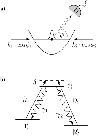
Figure 1: a) Geometry of the lasers and position of the detector with respect to the axis $x$ of the atomic center–of–mass motion. We denote with $k_{1}\cos\phi_{1}$ and $k_{2}\cos\phi_{2}$ the projections of the laser wave vectors on the $x$-axis. The detector D records the light scattered at an angle $\psi$ with respect to the motional axis. b) Relevant electronic transitions. The stable or metastable states $|\,1\,\rangle$ and $|\,2\,\rangle$ are coupled by dipole transitions to the excited state $|\,3\,\rangle$. The lasers drive the transition $|\,j\,\rangle\to|\,3\,\rangle$ with Rabi frequency $\Omega_{j}$ and both are tuned from resonance by $\delta$. The state $|\,3\,\rangle$ decays with rate $\gamma_{j}$ into $|\,j\,\rangle$ ($j=1,2$).

In the Lamb–Dicke regime, the dynamics of the driven atom can be described by a hierarchy of processes at the different orders in the ratio $\Delta x/\lambda_{L}$, which accounts for the effects of the field spatial gradient over the center–of–mass wave packet. At zero order in $\Delta x/\lambda_{L}$, internal and external degrees of freedom are decoupled, and the internal stationary state of the atom is the dark state CPT

$$|\psi_{\rm D}\rangle=\frac{\Omega_{2}|1\rangle-\Omega_{1}|2\rangle}{\sqrt{\Omega_{1}^{2}+\Omega_{2}^{2}}},$$ (2)

with the Rabi frequency ${\Omega_{j}={\bf d}_{j}\cdot\mbox{\boldmath$\epsilon$}_{j}{\cal E}_{j}/\hbar}$, which we assume to be real. In this limit, at steady state the density matrix of the atom is the product $\rho_{\rm D}\mu$ of the density matrix for the external degrees of freedom $\mu$ and for the internal degrees of freedom $\rho_{\rm D}=|\psi_{\rm D}\rangle\langle\psi_{\rm D}|$.

At first order in $\Delta x/\lambda_{L}$ the state $|\psi_{\rm D}\rangle$ becomes unstable due to the spatial gradient of the field over the finite size of the wave packet: Therefore, at steady state the density matrix of the atom is $\rho_{\rm st}=\rho_{\rm D}\mu+{\rm O}(\Delta x/\lambda_{L})$, where the correction ${\rm O}(\Delta x/\lambda_{L})$ accounts for the processes due to the mechanical effects of the coupling between light and atom.

The dynamics of this system has been investigated in Giovanna03 in the context of laser-cooling. There, it has been characterized by two main time scales: A faster time scale $T_{0}$, for the scattering processes at zero order in $\Delta x/\lambda_{L}$, where internal and external degrees of freedom are decoupled, and a slower time scale $T_{1}\gg T_{0}$, where the effects due to the field gradient along the center–of–mass wave packet manifest. On the time scale $T_{0}$ the internal dynamics accesses the dark state $|\,\psi_{D}\,\rangle$, and the atom ceases to scatter photons. On the time scale $T_{1}$, the atom absorbs light that is out of phase with the laser field due to the harmonic motion, thereby leaving the dark state and undergoing transitions that change the vibrational state. Then, light is scattered at zero order in $\Delta x/\lambda_{L}$ and the atom reaccesses the dark state. In other words, on a coarse–grained dynamics the internal state of the atom is $\rho_{\rm D}$, whereas the correction term ${\rm O}(\Delta x/\lambda_{L})$ in $\rho_{\rm st}$ accounts for the processes which couple internal and external degrees of freedom, and give rise to the spectrum of emission.

In Fig. 2 two spectra of emission of the dipole ${\bf d_{1}}$ Footnote are shown for (a) $\Delta x/\lambda_{L}\approx 7\times 10^{-4}$ and (b) $\Delta x/\lambda_{L}\approx 4\times 10^{-3}$. The most striking feature is the visibility of the sidebands of the elastic peak, namely the two signals at $\omega_{L,1}\pm\nu$, compared to the rest of the spectrum. These motional sidebands are Lorentz curves of equal height, and their functional dependence on the frequency is plotted in the insets of Fig. 2. They originate from Raman scattering processes, where the initial and final state is $|\psi_{\rm D}\rangle$ and the vibrational state is changed by one phonon. These processes occur on the time scale $T_{1}$, which also determines the linewidth of the resonances.

The broad signals of the spectrum correspond to the Mollow—type inelastic spectrum Narducci90 ; Plenio95 and their typical height is orders of magnitude smaller than the height of the motional sidebands for $\Delta x/\lambda_{L}\approx 7\times 10^{-4}$, while it is comparable for $\Delta x/\lambda\approx 4\times 10^{-3}$. We remark that the intensity of the elastic peak is at higher order in $\Delta x/\lambda_{L}$. In the following, we evaluate and discuss the spectrum in detail.

Figure 2: Spectrum of resonance fluorescence $S(\omega)$ (in arbitrary units) as a function of the frequency $\omega-\omega_{L,1}$ in units of $\nu$. The parameters are $\Omega_{1}=\Omega_{2}=8.5\nu$, $\gamma=10\nu$, $\gamma_{1}=\gamma_{2}$, $\delta=35\nu$, $\phi_{1}=0$, $\phi_{2}=\pi$, corresponding to $\langle n\rangle=0.005$. In a) $\eta_{1}=\eta_{2}=0.01$, in b) $\eta_{1}=\eta_{2}=0.05$. In both figures, the insets show the details of the curves at $\omega=\omega_{L,1}\pm\nu$. The contributions to the spectrum are plotted separately: The solid line corresponds to the signal of the Stokes and anti-Stokes components, the dashed line to the signal due to the Mollow–type inelastic spectrum.

III Evaluation of the spectrum of resonance fluorescence

Let the detector measure the radiation scattered by the dipole ${\bf d_{1}}$ Footnote . In the far–field the spectrum at frequency $\omega$ is determined by ${\cal S}(\omega)=\chi S(\omega)$, where $\chi$ collects all prefactors which do not depend on $\omega$. All results are rescaled by this common factor, which contains the dipole radiation pattern and is therefore a function of $\psi$. At a different angle than the laser propagation directions, the expression

$$S(\omega)={\rm Re}\int_{0}^{\infty}{\rm d}\tau{\rm e}^{-{\rm i}(\omega-\omega_{L,1})\tau}\langle D^{\dagger}(x,\tau)D(x,0)\rangle$$ (3)

contains the frequency dependence, where $D(x,t)$ is the generalized dipole lowering operator for the transition $|\,1\,\rangle\to|\,3\,\rangle$ in the reference frame rotating with the laser frequency $\omega_{L,1}$. By means of the quantum regression theorem, the two–time correlation function in Eq. (3) is determined by the Liouvillian ${\cal L}$ defined in the master equation $\partial\rho/\partial t={\cal L}\rho$ for the atomic dynamics Carmichael93 . Thus, the dipole lowering operator at time $t$ in Eq. (3) is given by $D(x,t)=D(x){\rm e}^{{\cal L}t}$ with $D(x)={\rm e}^{-{\rm i}k_{1}x\cos\psi}|1\rangle\langle 3|$. Here, the center-of-mass position $x$ is an operator acting on the atomic external degrees of freedom. The average $\langle\cdot\rangle$ is taken over the atomic density matrix $\rho_{\rm st}$ at steady state, given by ${\cal L}\rho_{\rm st}=0$.

We evaluate $S(\omega)$, Eq. (3), by applying the spectral decomposition of the Liouville operator ${\cal L}$ Briegel93 ; Barnett2000 according to the secular equations

$${\cal L}\rho^{\lambda} = \lambda\rho^{\lambda},$$

$$\check{\rho}^{\lambda}{\cal L} = \lambda\check{\rho}^{\lambda},$$

with eigenvalues $\lambda$ and right and left eigenelements $\rho^{\lambda}$ and $\check{\rho}^{\lambda}$, respectively. The orthogonality and completeness of the eigenelements is defined with respect to the trace, such that ${\rm Tr}\{\check{\rho}^{\lambda^{\prime}}\rho^{\lambda}\}=\delta_{\lambda^{\prime},\lambda}$, where any density operator $\rho$ can be decomposed as $\rho=\sum_{\lambda}\rho^{\lambda}{\rm Tr}\{\check{\rho}^{\lambda}\rho\}$ FootnoteCompleteness . We define the projectors onto the eigenspace corresponding to the eigenvalue $\lambda$ as ${\cal P}^{\lambda}=\rho^{\lambda}\otimes\check{\rho}^{\lambda}$ leading to

$${\cal L}{\cal P}^{\lambda}={\cal P}^{\lambda}{\cal L}=\lambda{\cal P}^{\lambda}.$$ (4)

Their action on an operator $X$ is defined as ${\cal P}^{\lambda}X=\rho^{\lambda}{\rm Tr}\{\check{\rho}^{\lambda}X\}$. By applying this formalism, we rewrite Eq. (3) as

$$S(\omega)={\rm Re}\sum_{\lambda}\frac{1}{{\rm i}(\omega-\omega_{L,1})-\lambda}{\rm Tr}\left\{D^{\dagger}(x){\cal P}^{\lambda}D(x)\rho_{\rm st}\right\}.$$ (5)

Hence, the spectrum of resonance fluorescence is the sum of Lorentz and/or Fano–like profiles, centered at the imaginary part of the eigenvalues of ${\cal L}$, with width given by the real part of $\lambda$. The exact evaluation of the spectrum for this kind of problem, with an infinite number of degrees of freedom, is a hard task. Nevertheless, an analytic solution can be found in the Lamb–Dicke regime. In this limit, we make perturbation theory in the parameter $\Delta x/\lambda_{L}$ on a spectral decomposition of ${\cal L}$, of which the spectrum $\{\lambda\}$ and the respective eigenelements at zero order are known.

III.1 Theoretical description

The master equation for the atomic dynamics reads

$$\frac{\partial}{\partial t}\rho(t)={\cal L}\rho(t)=\frac{1}{{\rm i}\hbar}[H,\rho(t)]+{\cal K}\rho(t),$$ (6)

where $H$ is the Hamilton operator for the coherent dynamics and ${\cal K}$ is the Liouvillian describing spontaneous emission. We decompose the Hamilton operator as

$$H=H_{\rm mec}+H_{0}+V(x),$$

where $H_{0}=\hbar\delta\sum_{j=1,2}|j\rangle\langle j|$ gives the eigenenergies of the electronic states in the reference frame of the laser, with $\delta=\omega_{L,1}-\omega_{1}=\omega_{L,2}-\omega_{2}$, where $\omega_{j}$ denotes the frequency of the transition $|\,j\,\rangle\to|\,3\,\rangle$. The term $H_{\rm mec}$ describes the center of mass motion of the atom with mass $M$ in a harmonic potential of frequency $\nu$,

$$H_{\rm mec}=\frac{p^{2}}{2M}+\frac{1}{2}M\nu^{2}x^{2}=\hbar\nu\left(a^{\dagger}a+\frac{1}{2}\right),$$ (7)

where $x$ and $p$ are the canonical conjugate variables describing position and momentum of the atom, whereas $a$ and $a^{\dagger}$ are the annihilation, creation operators of a quantum of energy $\hbar\nu$, respectively, such that $x=\sqrt{\hbar/2M\nu}(a+a^{\dagger})$, and $p={\rm i}\sqrt{\hbar M\nu/2}(a^{\dagger}-a)$. We denote with $|n\rangle$ the eigenelements of $H_{\rm mec}$, fulfilling $H_{\rm mec}|n\rangle=\hbar\nu(n+1/2)|n\rangle$ with $n=0,1,2,\ldots$

The term $V(x)$ describes the coherent interaction of the atom with the lasers at the position $x$ of the center of mass,

$$V(x)=\frac{1}{2}\sum\limits_{j=1,3}\hbar\Omega_{j}\left({\rm e}^{-{\rm i}k_{j}\cos\phi_{j}x}|3\rangle\langle j|+{\rm h.c.}\right),$$ (8)

and the exponentials account for the recoil momenta $\pm\hbar k_{j}\cos\phi_{j}$ of the atom when absorbing or emitting a photon. The operator ${\cal K}$ in Eq. (6) describes the spontaneous decay, according to

$${\cal K}\rho(t)= -\frac{\gamma}{2}\left(|\,3\,\rangle\langle\,3\,|\rho(t)+\rho(t)|\,3\,\rangle\langle\,3\,|\right)$$ (9)

$$+\sum\limits_{j=1,2}\gamma_{j}|\,j\,\rangle\langle\,3\,|\tilde{\rho}_{j}(t)|\,3\,\rangle\langle\,j\,|,$$

where $\gamma_{1}+\gamma_{2}=\gamma$. Here, we have introduced

$$\tilde{\rho}_{j}(t)=\int\limits_{-1}^{1}{\rm d}\!\cos\!\theta\,{\cal N}(\cos\!\theta)\,{\rm e}^{ik_{j}x\cos\theta}\rho(t)\;{\rm e}^{-ik_{j}x\cos\theta},$$ (10)

which describes the momentum transfer $\hbar k_{j}\cos\theta$ due to the photons spontaneously emitted at angle $\theta$ with respect to the motional axis and with angular distribution ${\cal N}(\cos\theta)$.

III.2 Perturbative expansion in the Lamb–Dicke parameter

In the Lamb–Dicke regime we can approximate $\exp\left(\pm{\rm i}k_{j}x\cos\varphi\right)=(1-\eta_{j}^{2}\cos^{2}\varphi/2(2a^{\dagger}a+1))\pm{\rm i}\eta_{j}\cos\varphi(a^{\dagger}+a)+{\rm O}(\eta_{j}^{3})$, where

$$\eta_{j}=\sqrt{\frac{\hbar k_{j}^{2}}{2M\nu}}$$

is the Lamb–Dicke parameter, corresponding to the ratio of the size of the oscillator ground state over the laser wavelength. Here, $\eta_{j}$ is the parameter of the perturbative expansion, and it fulfills the relation $\eta_{j}\sqrt{2\langle n\rangle+1}\approx\Delta x/\lambda_{L}\ll 1$. In second order in $\eta_{j}$ expression (5) has the form

$$S(\omega)=S_{0}(\omega)+S_{1}(\omega)+S_{2}(\omega)+{\rm O}(\eta_{j}^{3}),$$ (11)

where the subscript $\alpha=0,1,2$ indicates the corresponding order in the perturbative expansion. In order to evaluate $S_{\alpha}(\omega)$, we expand the operators ${\cal L}$ and $D$ in power of $\eta_{j}$, yielding

$$D_{0}=|1\rangle\langle 3|,$$

$$D_{1}=-{\rm i}k_{1}x\cos\psi|1\rangle\langle 3|,$$

$$D_{2}=-\frac{1}{2}k_{1}^{2}x^{2}\cos^{2}\psi|1\rangle\langle 3|,$$

and

$${\cal L}_{0}\rho = \frac{1}{{\rm i}\hbar}[H_{\rm mec},\rho]+\frac{1}{{\rm i}\hbar}[H_{0}+V(0),\rho]+{\cal K}_{0}\rho$$ (12)

$$= ({\cal L}_{E}+{\cal L}_{I})\rho,$$

$${\cal L}_{1}\rho = \frac{1}{{\rm i}\hbar}\left[V_{1}x,\rho\right],$$ (13)

$${\cal L}_{2}\rho = \frac{1}{2{\rm i}\hbar}\left[V_{2}x^{2},\rho\right]+{\cal K}_{2}\rho.$$ (14)

In Eq. (12) we have introduced the Liouville operators ${\cal L}_{E}$ and ${\cal L}_{I}$, which account for the external and internal degrees of freedom. They are defined as ${\cal L}_{E}\rho=1/{\rm i}\hbar\left[H_{\rm mec},\rho\right]$ and ${\cal L}_{I}\rho=1/{\rm i}\hbar\left[H_{0}+V(0),\rho\right]+{\cal K}_{0}\rho$.

By determining ${\cal L}_{\alpha}$, we have used the expansion of the interaction term, Eq. (8), $V(x)=V(0)+V_{1}x+V_{2}x^{2}/2+{\rm O}(\eta_{j}^{3})$ with

$$V_{\alpha}=\frac{\partial^{\alpha}}{\partial x^{\alpha}}V(x)\Bigl{|}_{x=0},~{}\alpha=1,2$$ (15)

and the expansion of Eq. (9), yielding

$${\cal K}_{0}\rho=\sum\limits_{j=1,2}\frac{\gamma_{j}}{2}\left(2|\,j\,\rangle\langle\,3\,|\rho|\,3\,\rangle\langle\,j\,|-|\,3\,\rangle\langle\,3\,|\rho-\rho|\,3\,\rangle\langle\,3\,|\right),$$

$${\cal K}_{2}\rho=\beta\sum\limits_{j=1,2}\gamma_{j}k_{j}^{2}\;|\,j\,\rangle\langle\,3\,|\left(2x\rho x-x^{2}\rho-\rho x^{2}\right)|\,3\,\rangle\langle\,j\,|.$$

Here, $\beta=\int_{-1}^{+1}{\rm d}\!\cos\!\theta~{}{\cal N}(\cos\!\theta)\cos^{2}\!\theta$ is a constant. We remark that the first order term ${\cal K}_{1}$ vanishes after averaging over the angles of emission $\theta$.

From Eq. (12) it can be seen that internal and external degrees of freedom are decoupled at zero order. Hence, the eigenvalues of ${\cal L}_{0}$ are

$$\lambda_{0}=\lambda_{E}+\lambda_{I},$$ (16)

with $\lambda_{E}$ and $\lambda_{I}$ being the eigenvalues of ${\cal L}_{E}$ and ${\cal L}_{I}$, respectively. The projector ${\cal P}^{\lambda}_{0}$ in the corresponding eigenspace factorizes into the projectors ${\cal P}^{\lambda_{I}}_{I}$ and ${\cal P}^{\lambda_{E}}_{E}$ assigned to the internal and external degrees of freedom, according to

$${\cal P}^{\lambda}_{0}={\cal P}^{\lambda_{I}}_{I}{\cal P}^{\lambda_{E}}_{E}.$$ (17)

The spectrum of ${\cal L}_{I}$ characterizes the dynamics of the three-level transition and the spectral properties of the radiation emitted by the bare atom. The eigenvalues of ${\cal L}_{E}$ take on the values $\lambda_{E}={\rm i}\ell\nu$, with $\ell=0,\pm 1,\pm 2,\ldots$ Each eigenspace at $\lambda_{E}$ is infinitely degenerate, and the corresponding left and right eigenelements are, for instance, $\check{\mu}_{n}^{\ell}=|n+\ell\rangle\langle n|$, $\mu^{\ell}_{n}=|n\rangle\langle n+\ell|$. These eigenelements constitute a complete and orthonormal basis over the eigenspace at this eigenvalue. In particular, the projector over the eigenspace at $\lambda_{E}={\rm i}\ell\nu$ is defined on an operator $X$ as

$${\cal P}^{\lambda_{E}={\rm i}\ell\nu}_{E}X = \sum_{n}\mu^{\ell}_{n}{\rm Tr}_{E}\{\check{\mu}_{n}^{\ell}X\}$$

$$= \sum_{n}|n\rangle\langle n|X|n+\ell\rangle\langle n+\ell|,$$

where ${\rm Tr}_{E}$ denotes the trace over the external degrees of freedom.

At first order in the expansion in $\eta_{j}$, internal and external degrees of freedom are coupled, and the degeneracy of the subspaces at eigenvalue $\lambda_{E}$ is lifted Lindberg84 ; Stenholm86 . The perturbative corrections to the eigenvalues $\lambda_{0}$, to the eigenelements $\rho^{\lambda}_{0}$, $\check{\rho}^{\lambda}_{0}$, and to the projectors ${\cal P}^{\lambda}_{0}$ are found by solving iteratively the secular equations at the same order $p$ in the perturbative expansion, that is

$$\sum_{\alpha=0}^{p}{\cal L}_{\alpha}\rho^{\lambda}_{p-\alpha}=\sum_{\alpha=0}^{p}\lambda_{\alpha}\rho^{\lambda}_{p-\alpha},$$ (19)

$$\sum_{\alpha=0}^{p}\check{\rho}^{\lambda}_{p-\alpha}{\cal L}_{\alpha}=\sum_{\alpha=0}^{p}\lambda_{\alpha}\check{\rho}^{\lambda}_{p-\alpha},$$ (20)

where $\rho_{\alpha}^{\lambda}$ and $\check{\rho}_{\alpha}^{\lambda}$ are the $\alpha$–order corrections to the eigenelements $\rho_{0}^{\lambda}$ and $\check{\rho}_{0}^{\lambda}$. The explicit forms up to second order are derived in Appendix A. In particular, $\rho_{0}^{\lambda=0}=\rho_{\rm D}\mu$ is the steady-state density matrix at zero order, where $\mu$ is the density matrix for the external degrees of freedom in the final stage of the laser–cooling dynamics Footnote:mu , and has the form

$$\mu=\frac{1}{1+\langle n\rangle}\left(\frac{\langle n\rangle}{1+\langle n\rangle}\right)^{a^{\dagger}a},$$ (21)

where

$$\langle n\rangle={\rm Tr}\{a^{\dagger}a\mu\}$$ (22)

is the average phonon number at steady state.

By substituting the explicit form of the operators into Eq. (5), we find that the zero– and first–order contributions to the spectrum vanish (see discussion in Appendix B), yielding

$$S(\omega)=S_{2}(\omega)+{\rm O}(\eta_{j}^{3}),$$ (23)

with

$$S_{2}(\omega)=\sum_{\lambda}\frac{g(\lambda)}{{\rm i}(\omega-\omega_{L,1})-\lambda}.$$ (24)

Here, $g(\lambda)$ is a complex-valued function, which we decompose for convenience into $g(\lambda)=f^{(1)}(\lambda)+f^{(2)}(\lambda)$, with

$$f^{(1)}(\lambda)={\rm Tr}\{D_{0}^{\dagger}{\cal P}_{1}^{\lambda}D_{0}\rho_{1}\},$$

$$f^{(2)}(\lambda)={\rm Tr}\{D_{0}^{\dagger}{\cal P}_{0}^{\lambda}D_{0}\rho_{2}\}.$$

Using $\rho_{1}^{\lambda}$, $\rho_{2}^{\lambda}$ and ${\cal P}_{1}^{\lambda}$, evaluated in Appendix A, and making use of relation (17), we separate the trace terms $f^{(1)}$ and $f^{(2)}$ into the product of the trace over the external and over the internal (${\rm Tr}_{I}\{\}$) degrees of freedom. By applying the cyclic properties of the trace and the the completeness relation for the external degrees of freedom, $\sum_{\lambda_{E}}P_{E}^{\lambda_{E}}=\mathbb{1}_{E}$, we find

$$f^{(1)}(\lambda)=\frac{1}{\hbar^{2}}\sum_{\lambda_{E}^{\prime}}\Bigl{[}\delta_{\lambda_{E},0}{\rm Tr}_{E}\left\{({\cal P}_{E}^{\lambda_{E}^{\prime}}[x,\mu])x\right\}$$

$$\times{\rm Tr}_{I}\left\{D_{0}^{\dagger}{\cal P}^{\lambda_{I}}_{I}\left[V_{1},\frac{1}{\lambda_{0}-\lambda_{E}^{\prime}-{\cal L}_{I}}D_{0}\frac{1}{\lambda_{E}^{\prime}+{\cal L}_{I}}V_{1}\rho_{\rm D}\right]\right\}$$

$$+\delta_{\lambda_{E},0}{\rm Tr}_{E}\left\{({\cal P}_{E}^{\lambda_{E}^{\prime}}\mu x)x\right\}$$

$$\times{\rm Tr}_{I}\left\{D_{0}^{\dagger}{\cal P}^{\lambda_{I}}_{I}\left[V_{1},\frac{1}{\lambda_{0}-\lambda_{E}^{\prime}-{\cal L}_{I}}D_{0}\frac{1}{\lambda_{E}^{\prime}+{\cal L}_{I}}[V_{1},\rho_{\rm D}]\right]\right\}$$

$$+\delta_{\lambda_{E}^{\prime},0}{\rm Tr}_{E}\left\{({\cal P}_{E}^{\lambda_{E}}[x,\mu])x\right\}$$

$$\times{\rm Tr}_{I}\left\{D_{0}^{\dagger}\frac{1}{\lambda_{0}-{\cal L}_{I}}\left[V_{1},{\cal P}^{\lambda_{I}}_{I}D_{0}\frac{1}{\lambda_{E}+{\cal L}_{I}}V_{1}\rho_{\rm D}\right]\right\}$$

$$+\delta_{\lambda_{E}^{\prime},0}{\rm Tr}_{E}\left\{({\cal P}_{E}^{\lambda_{E}}\mu x)x\right\}$$

$$\times{\rm Tr}_{I}\left\{D_{0}^{\dagger}\frac{1}{\lambda_{0}-{\cal L}_{I}}\left[V_{1},{\cal P}^{\lambda_{I}}_{I}D_{0}\frac{1}{\lambda_{E}+{\cal L}_{I}}[V_{1},\rho_{\rm D}]\right]\right\}\Big{]},$$

where we have used the relation ${\rm Tr}_{E}\{P^{\lambda_{E}}_{E}X\}=\delta_{\lambda_{E},0}{\rm Tr}_{E}\{X\}$. Analogously,

$$f^{(2)}(\lambda)=-\frac{1}{\hbar^{2}}\delta_{\lambda_{E},0}\sum_{\lambda_{E}^{\prime}}\Bigl{[}{\rm Tr}_{E}\{({\cal P}_{E}^{\lambda_{E}^{\prime}}\mu x)x\}$$

$$\times{\rm Tr}_{I}\left\{D_{0}^{\dagger}{\cal P}_{I}^{\lambda_{I}}D_{0}{\cal L}_{I}^{-1}\left[V_{1},\left(\frac{1}{\lambda_{E}^{\prime}+{\cal L}_{I}}[V_{1},\rho_{\rm D}]\right)\right]\right\}$$

$$+{\rm Tr}_{E}\{({\cal P}_{E}^{\lambda_{E}^{\prime}}[x,\mu])x\}$$

$$\times{\rm Tr}_{I}\left\{D_{0}^{\dagger}{\cal P}_{I}^{\lambda_{I}}D_{0}{\cal L}_{I}^{-1}\left[V_{1},\left(\frac{1}{\lambda_{E}^{\prime}+{\cal L}_{I}}V_{1}\rho_{\rm D}\right)\right]\right\}\Big{]}$$

$$-\frac{\rm i}{2\hbar}\delta_{{\lambda_{E}},0}{\rm Tr}_{E}\{\mu x^{2}\}{\rm Tr}_{I}\left\{D_{0}^{\dagger}{\cal P}_{I}^{\lambda_{I}}D_{0}{\cal L}_{I}^{-1}[V_{2},\rho_{D}]\right\}.$$

From the properties of the terms ${\rm Tr}_{E}\{X\}$ one can already see that the eigenelements and eigenvalues of ${\cal L}_{E}$ contributing to the spectrum at second order are at $\lambda_{E}=0,\pm{\rm i}\nu$.

In summary, the first non-vanishing contribution to the spectrum of emission is in second order in the perturbative expansion. It can be decomposed into the sum of curves, centered at the imaginary part of the eigenvalues $\lambda$ of the Liouville operator ${\cal L}$, and weighted by the factor $g(\lambda)$. The eigenvalues are here determined up to the second order correction, $\lambda=\lambda_{0}+\lambda_{2}+{\rm O}(\eta_{j}^{3})$, whereby $\lambda_{1}=0$, as shown in Appendix A and in Lindberg84 . At zero order in the perturbative expansion $\lambda_{0}=\lambda_{I}+\lambda_{E}$, where $\lambda_{I}$ is the eigenvalue of the Liouvillian of a bare $\Lambda$–transition, while the only relevant external eigenvalues are $\lambda_{E}=0,\pm{\rm i}\nu$.

Below, we analyze the spectrum in detail. For later convenience, we rewrite $S(\omega)=S_{\rm el}(\omega)+S_{\rm M}(\omega)+S_{\rm SB}(\omega)$, where $S_{\rm el}(\omega)$ is the contribution of the elastic peak, at $\lambda=0$, the term

$$S_{\rm M}(\omega)=\sum\limits_{\lambda_{I}\neq 0,\lambda_{E}}\frac{g(\lambda)}{{\rm i}(\omega-\omega_{L,1})-\lambda}$$ (25)

denotes the contributions at $\lambda_{I}\neq 0$, which we refer to as the Mollow–type inelastic component Narducci90 ; Plenio95 . The term

$$S_{\rm SB}(\omega)=\sum\limits_{\lambda_{I}=0,\atop\lambda_{E}=\pm{\rm i}\nu}\frac{g(\lambda)}{{\rm i}(\omega-\omega_{L,1})-\lambda}$$ (26)

represents the contributions at $\lambda_{I}=0,\lambda_{E}=\pm{\rm i}\nu$, that we identify with the sidebands of the elastic peak, or Stokes-, anti-Stokes components of the scattered radiation.

We remark that $S_{2}(\omega)$ does not depend on the position of the detector: the terms containing the perturbative corrections $D_{1}$, $D_{2}$ and their adjoints do not contribute to $S(\omega)$ in second order in $\eta_{j}$. Furthermore, the Lamb–Dicke parameters $\eta_{1}$, $\eta_{2}$ appear always in the form $\eta_{1}\cos\phi_{1}$, $\eta_{2}\cos\phi_{2}$, since ${\cal K}_{2}\rho_{0}^{\lambda=0}\propto{\cal K}_{2}\rho_{\rm D}=0$ (see Appendix B). Therefore, the mechanical effects in second order are solely determined by the scattering of laser photons and not by recoils due to spontaneously emitted photons. This behaviour is due to destructive quantum interference at zero order in the Lamb–Dicke expansion, implying that light absorption is a first-order process Giovanna03 ; FootnoteN .

III.2.1 The Mollow–type inelastic spectrum

At zero order in the Lamb–Dicke parameter, the eigenvalues $\lambda_{I}\neq 0$ determine the position and the shape of the contributions to the Mollow–type inelastic spectrum. As $\lambda$ appears in the denominator of $S_{\rm M}(\omega)$, the second-order correction $\lambda_{2}$ can be neglected.

The trace terms over the external degrees of freedom are conveniently evaluated using the basis set corresponding to the projectors in Eq. (III.2), giving

$${\rm Tr}_{E}\{({\cal P}_{E}^{\lambda_{E}}\mu x)x\}=x_{0}^{2}\left[\delta_{{\lambda_{E}},{\rm i}\nu}(\langle n\rangle+1)+\delta_{{\lambda_{E}},-{\rm i}\nu}\langle n\rangle\right],$$

$${\rm Tr}_{E}\{({\cal P}_{E}^{\lambda_{E}}[x,\mu])x\}=x_{0}^{2}\left[-\delta_{{\lambda_{E}},{\rm i}\nu}+\delta_{{\lambda_{E}},-{\rm i}\nu}\right],$$

$${\rm Tr}_{E}\{x^{2}\mu\}=x_{0}^{2}\left[2\langle n\rangle+1\right],$$ (27)

with $x_{0}=\sqrt{\hbar/2M\nu}$. Thus, at second order in the Lamb–Dicke expansion the eigenelements of ${\cal L}_{E}$ determining the spectrum are in the eigenspaces corresponding to $\lambda_{E}=0,\pm{\rm i}\nu$. Since $S_{\rm M}(\omega)$ is linear in these terms, this component of the spectrum scales with $\eta_{j}^{2}\cos^{2}\phi_{j}$ and is linear in the average phonon number $\langle n\rangle$.

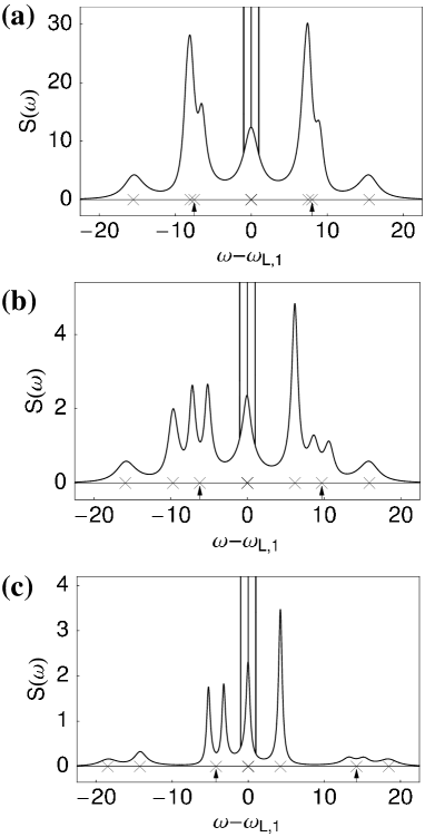
Figure 3: Spectrum $S(\omega)$ in arbitrary units as a function of $\omega-\omega_{L,1}$ in units of $\nu$. The figures are at different values of the detuning $\delta$, for $\Omega_{1}=\Omega_{2}=10\nu$, $\gamma=5\nu$, $\gamma_{1}=\gamma_{2}$, $\phi_{1}=0,\phi_{2}=\pi$, $\eta_{1}=\eta_{2}=10^{-4}$. (a) $\delta=0.5\nu$, corresponding to $\langle n\rangle=30$. (b) $\delta=3.5\nu$, corresponding to $\langle n\rangle=3.8$. (c) $\delta=10\nu$, corresponding to $\langle n\rangle=1$. In all figures, the crosses on the frequency axis indicate the positions of the frequencies ${\rm Im}\{\lambda_{I}\}$. The arrows indicate the frequencies ${\rm Im}\{\lambda_{I}^{\prime}\}$ of which only the sidebands appear in the spectrum.

This spectral component is constituted by the contributions of the signals centered at ${\rm Im}\{\lambda_{I}\}$ and at ${\rm Im}\{\lambda_{I}^{\prime}\}\pm\nu$. The latter originate from the term $f^{(1)}(\lambda)$ in $g(\lambda)$. We illustrate this behaviour in Fig. 3, where the Mollow–type inelastic spectrum is shown for different values of the detuning $\delta$ (and correspondingly of the average phonon number at steady state $\langle n\rangle$). The frequencies ${\rm Im}\{\lambda_{I}\}$ are marked with crosses on the frequency axis, where the arrows indicate the center–frequencies ${\rm Im}\{\lambda_{I}^{\prime}\}$ of which only the sidebands are visible. In order to highlight this splitting, we have taken borderline parameters, such that all peaks are clearly resolved. For realistic parameters, the sidebands on the left side of the spectrum are visible, as shown in Fig. 2(b).

The curves at ${\rm Im}\{\lambda_{I}\}$ can be reproduced by evaluating the spectrum of emission of a bare three-level atom, whose ground state coherence has a finite lifetime Narducci90 ; Plenio95 . Thus, they can be identified with the spectrum of the photons scattered at zero order in the Lamb–Dicke parameter. The signals centered at ${\rm Im}\{\lambda_{I}^{\prime}\}\pm\nu$ are peculiar. They correspond to processes where photon scattering is accompanied by a change in the vibrational state. Looking at the corresponding eigenelements, it follows that they stem from the inelastic processes which take the atom out of the dark state. We remark that in Fig. 2 the left pole ${\rm Im}\{\lambda_{I}^{\prime}\}$ falls at the same frequency as the left motional sideband: In fact, the parameters have been here chosen, so that the frequency of absorption along the cooling transition coincides with the narrow resonance characterizing the excitation spectrum EITcooling ; Giovanna03 ; Lounis92 .

III.2.2 The sidebands of the elastic peak

The spectral contributions at $\lambda_{I}=0$, $\lambda_{E}=\pm{\rm i}\nu$, allow for a compact analytic form. Only the term $f^{(1)}(\lambda)$ contributes to $g(\lambda)$ in $S_{\rm SB}(\omega)$. After some algebraic manipulation, we write

$$g(\lambda_{E})={\rm Tr}_{E}\left\{({\cal P}_{E}^{\lambda_{E}}(a+a^{\dagger})\mu)(a+a^{\dagger})\right\}|f(\lambda_{E})|^{2},$$

where

$$f(\lambda_{E})=\frac{x_{0}}{\hbar}{\rm Tr}_{I}\{D_{0}^{\dagger}\frac{1}{\lambda_{E}-{\cal L}_{I}}[V_{1},\rho_{D}]\}.$$ (28)

The explicit form (28) is found by applying the relation $(\lambda-{\cal L}_{I})^{-1}=\int\limits_{0}^{\infty}{\rm d}t\,{\rm e}^{-(\lambda-{\cal L}_{I})t}$. Using the quantum regression theorem we arrive at

$$f(\lambda_{E})=-{\rm i}\frac{2\eta\lambda_{E}\Omega_{1}\Omega_{2}^{2}}{\Omega^{2}(\Omega^{2}+4\lambda_{E}({\rm i}\delta+\lambda_{E}+\gamma/2))},$$ (29)

with $\Omega^{2}=\Omega_{1}^{2}+\Omega_{2}^{2}$, and where we have introduced $\eta=x_{0}(k_{1}\cos\phi_{1}-k_{2}\cos\phi_{2})$. The explicit form of $S_{\rm SB}(\omega)$ is determined after evaluating the second order corrections $\lambda_{2}$ to $\lambda_{0}=\pm{\rm i}\nu$. These are found by solving the eigenvalue equations (38) and (39) at $\lambda_{0}=\pm{\rm i}\nu$. In the subspace at $\lambda_{E}={\rm i}\ell\nu$, $\lambda_{I}=0$, after tracing over the internal degrees of freedom, they read

$$\lambda_{2}\tilde{\mu}^{\lambda_{2}} = s(\nu)\left[a\tilde{\mu}^{\lambda_{2}}a^{\dagger}-a^{\dagger}a\tilde{\mu}^{\lambda_{2}}\right]$$ (30)

$$+ s(-\nu)\left[a^{\dagger}\tilde{\mu}^{\lambda_{2}}a-aa^{\dagger}\tilde{\mu}^{\lambda_{2}}\right]+{\rm H.c.},$$

where $\tilde{\mu}^{\lambda_{2}}$ are the right eigenelements of Eq. (30) at the eigenvalue $\lambda_{2}$. The left eigenelements $\check{\tilde{\mu}}^{\lambda_{2}}$ fulfill the corresponding equation for the action to the left Briegel93 ; Barnett2000 . The coefficient $s(\nu)$ is given by

$$s(\nu) = \frac{1}{2M\nu}\int\limits_{0}^{\infty}{\rm d}t\,{\rm e}^{{\rm i}\nu t}{\rm Tr}_{I}\{V_{1}{\rm e}^{{\cal L}_{I}t}V_{1}\rho_{D}\}$$ (31)

$$= \eta^{2}\frac{{\rm i}\nu\Omega_{1}^{2}\Omega_{2}^{2}}{\Omega^{2}(\Omega^{2}+4\nu({\rm i}\gamma/2-\nu+\delta))}.$$

We rewrite $s(\pm\nu)={\rm Re}[s(\pm\nu)]+{\rm i}~{}{\rm Im}[s(\pm\nu)]$, and define $A_{\pm}=2{\rm Re}\{s(\mp\nu)\}$. Substituting into Eq. (30), we obtain the more familiar form Stenholm86 ; Briegel93

$$\lambda_{2}\tilde{\mu}^{\lambda_{2}} = -i\bar{\nu}[a^{\dagger}a,\tilde{\mu}^{\lambda_{2}}]$$

$$+A_{-}\left[2a\tilde{\mu}^{\lambda_{2}}a^{\dagger}-a^{\dagger}a\tilde{\mu}^{\lambda_{2}}-\tilde{\mu}^{\lambda_{2}}a^{\dagger}a\right]$$

$$+A_{+}\left[2a^{\dagger}\tilde{\mu}^{\lambda_{2}}a-aa^{\dagger}\tilde{\mu}^{\lambda_{2}}-\tilde{\mu}^{\lambda_{2}}aa^{\dagger}\right],$$

with $\bar{\nu}={\rm Im}[S(\nu)]+{\rm Im}[S(-\nu)]$. The corresponding eigenvalues are solutions of Eq. (45), and have the form Briegel93 ; Stenholm86 ; Lindberg84

$$\lambda_{2}(N,\ell)=-{\rm i}\ell\bar{\nu}-\left(2N+|\ell|\right)(A_{-}-A_{+}),$$ (33)

where the index $N=0,1,2,\ldots$ accounts for the removed degeneracy inside the eigenspace. The explicit form of the corresponding left and right eigenelements $\check{\tilde{\mu}}^{N,\ell}$, $\tilde{\mu}^{N,\ell}$ can be found in Briegel93 . They form a complete and orthogonal set with respect to the trace over the external degrees of freedom, ${\rm Tr}_{E}\{\check{\tilde{\mu}}^{N,\ell}\tilde{\mu}^{N^{\prime},\ell^{\prime}}\}=\delta_{N,{N^{\prime}}}\delta_{\ell,{\ell^{\prime}}}$ and $\sum_{N,\ell}\tilde{\mu}^{N,\ell}\otimes\check{\tilde{\mu}}^{N,\ell}=\mathbb{1}_{E}$. In particular, the eigenelements $\tilde{\mu}^{N,\ell}$, $\check{\tilde{\mu}}^{N,\ell}$ form a complete basis over the subspace at eigenvalue $\lambda_{E}={\rm i}\ell\nu$, such that

$${\cal P}_{E}^{\lambda_{E}={\rm i}\ell\nu}=\sum_{N}\tilde{\mu}^{N,\ell}\otimes\check{\tilde{\mu}}^{N,\ell}.$$

We remark that the density operator given in Eq. (21) is right eigenelement at $N=\ell=0$, that is $\mu=\tilde{\mu}^{0,0}$. Using this basis for evaluating the trace terms over the external degrees of freedom, we get

$$S_{\rm SB}(\omega)={\rm Re}\sum_{\ell,N}\frac{|f(\lambda_{E})|^{2}}{{\rm i}(\omega-\omega_{L,1}-\ell\nu)-\lambda_{2}^{N,\ell}}$$

$$\times~{}{\rm Tr}_{E}\{(a+a^{\dagger})\tilde{\mu}^{N,\ell}\}{\rm Tr}_{E}\{\check{\tilde{\mu}}^{N,\ell}(a+a^{\dagger})\mu\}.$$

By using the explicit form of the eigenelements in Briegel93 we find that only the terms at $N=0$, $\ell=\pm 1$ contribute to the sum, giving

$$S_{\rm SB}(\omega)=\sum_{\ell=\pm 1}\frac{\gamma_{\rm S}^{2}}{[\omega-\omega_{L,1}+\ell(\nu+\bar{\nu})]^{2}+\gamma_{\rm S}^{2}}~{}s_{0},$$ (34)

where $\gamma_{\rm S}=A_{-}-A_{+}$ and $s_{0}$ is the height at the center frequency and has the form footnoteOtherTransition

$$s_{0}=\frac{\nu\Omega_{1}^{2}\Omega_{2}^{4}}{4\tilde{\gamma}_{\rm S}\delta\Omega^{4}(\Omega^{2}-4\nu^{2})}.$$ (35)

Here, we have defined $\tilde{\gamma}_{\rm S}=\gamma_{\rm S}/\eta^{2}$, which is at zero order in the Lamb–Dicke expansion.

From Eq. (34) one sees that both sidebands of the elastic peak have the same form, independent of the angle $\psi$ of the detector with respect to the axis of the motion. In particular, they have the same Lorentzian shape, as shown in the insets of Fig. 2, and are centered at the frequency $\pm(\nu+\bar{\nu})$, where $\bar{\nu}$ is a shift in second order in the Lamb–Dicke parameter. We illustrate this effect in Fig. 4, where we have chosen suitable parameter to show this small shift most clearly. Here, $\bar{\nu}$ can be identified with the a.c.–Stark shift arising from off-resonant coupling to other dipole transitions at different vibrational numbers. The width $\gamma_{\rm S}$ of the sidebands is at second order in the Lamb–Dicke parameter and corresponds to the cooling rate Giovanna03 . The height $s_{0}$ is in zero order in the perturbative expansion. With some algebraic manipulations, using $\langle n\rangle=A_{+}/\gamma_{\rm S}$, it can be rewritten as

$$s_{0}=\frac{\Omega_{2}^{2}}{\gamma\Omega^{2}}\langle n\rangle(1+\langle n\rangle).$$ (36)

Thus, the motional sidebands are well distinguished compared to the Mollow–type inelastic spectrum for ${\eta^{2}\ll\langle n\rangle}$.

III.2.3 The elastic peak

The contribution at the eigenvalue $\lambda=0$ corresponds to the elastic peak, i.e. to the coherent part of the spectrum. In this system its appearance is due to the mechanical effects of light: In fact, at zero order in the Lamb–Dicke expansion there is no photon emission at steady state. We evaluate the radiation scattered at this frequency starting from expression (5),

$$S_{\rm el}(\omega)=\pi\delta(\omega-\omega_{L,1})\,{\rm Tr}\left\{D^{\dagger}{\cal P}^{\lambda=0}D\rho_{\rm st}\right\}$$

$$=\pi\delta(\omega-\omega_{L,1})\,|{\rm Tr}\left\{D^{\dagger}\rho_{\rm st}\right\}|^{2},$$ (37)

which is the well-known form of the elastic peak contribution AtomPhoton . The perturbative expansion of $D$ and $\rho_{\rm st}$ can now be applied for evaluating the average dipole moment ${\rm Tr}\{D\rho_{\rm st}\}$. We find the first non-vanishing contribution at O($\eta_{j}^{2}$), such that ${\rm Tr}\{D\rho_{\rm st}\}={\rm Tr}\{D_{0}^{\dagger}\rho_{2}\}+{\rm Tr}\{D_{1}^{\dagger}\rho_{1}\}+{\rm O}(\eta_{j}^{4})$. This signal is due to the lowest order corrections of the Debye–Waller factor, $\exp(-\eta_{j}^{2}\cos^{2}\phi_{j}/2)$, on the transitions $|\psi_{\rm D},n\rangle\to|3,n\rangle\to|\psi_{\rm D},n\rangle$, and to the coefficient $\eta_{j}^{2}n\cos\phi_{j}\cos\psi$ on the transitions $|\psi_{\rm D},n\rangle\to|3,n\pm 1\rangle\to|\psi_{\rm D},n\rangle$. Thus, the intensity of the radiation scattered at the elastic peak is at fourth order in the Lamb–Dicke parameter and it depends on the angle of emission. The finite life time of the dark state suggests also a broadened signal at this frequency. Our analysis shows that such contribution is of higher order in the perturbative expansion.

IV Summary of the results and discussion

The spectrum of emission of a trapped ion, whose internal degrees of freedom constitute a $\Lambda$–transition driven at two-photon resonance, is a remarkable manifestation of the mechanical effects of light: In fact, at steady state photons are emitted due to processes where the vibrational degrees of freedom are excited by absorption of a photon. We have evaluated the spectrum using perturbation theory in the Lamb–Dicke parameter. According to our results, the signal of the emission spectrum is in second order in the Lamb–Dicke expansion. We classify the spectral features into three main contributions, which we summarize below.

At the laser frequency $\omega_{L,1}$ the spectrum exhibits a $\delta$-peaked signal, visible for instance in Fig. 2, that we identify with the elastic peak. This signal is at fourth order in the perturbative expansion. This order of magnitude is understood, as the dipole moment at steady state scales with $\eta_{j}^{2}\sim(\Delta x/\lambda_{L})^{2}$. In fact, this signal is due to Rayleigh scattering processes where the initial and final state is the dark state $|\psi_{\rm D}\rangle$ and the vibrational number $n$ is conserved. Thus, this excitation originates from the lowest order mechanical corrections to the Rabi frequency and it depends on the angle of emission $\psi$.

At the frequencies $\omega_{L,1}\pm\nu$ one observes two narrow resonances. These are the motional sidebands of the elastic peak, the Stokes and anti-Stokes components of the scattered light. They correspond to Raman scattering where the initial and final internal state is $|\,\psi_{\rm D}\,\rangle$ and the vibrational number is changed by one phonon. The curves are Lorentz curves, whose dependence on the physical parameters is given by Eq. (34) and plotted in the insets of Fig. 2. Their width is in second order in the Lamb–Dicke expansion and corresponds with the cooling rate Stenholm86 . The height of the curves at the center frequency scales with the average phonon number $\langle n\rangle$ according to $\langle n\rangle(1+\langle n\rangle)$, so that the total intensity emitted at this frequency is proportional to $\eta^{2}\langle n\rangle$. Finally, the center frequencies of the sidebands are shifted from the zero–order center frequency by a contribution $\bar{\nu}$ at second order in the Lamb–Dicke expansion: This corresponds to the a.c.–Stark shift of the ground–state coherence due to the off-resonant coupling with the excited state. Figure 4 shows the shift $\bar{\nu}$ for one sideband.

Figure 4: Spectrum of resonance fluorescence $S(\omega)$ (in arbitrary units) as a function of the frequency $\omega-\omega_{L,1}$ in units of $\nu$. The parameters are $\phi_{1}=0$, $\phi_{2}=\pi$, $\eta_{1}=\eta_{2}=0.05$, $\Omega_{1}=\Omega_{2}=8.5\nu$, $\gamma=10\nu$, $\gamma_{1}=\gamma_{2}$, $\delta=15\nu$, corresponding to $\langle n\rangle=0.2$. In the onset, the Stokes component is shown: The vertical dashed line indicate the position of the frequency $\omega-\omega_{L,1}=-\nu$. In the inset, the whole spectrum is shown. The signal of the inelastic part is here two orders of magnitude smaller than the sidebands.

The other spectral features, visible for instance in Fig. 2(b), can be identified with the Mollow–type inelastic spectrum. These can be decomposed into the sum of Lorentz curves, whose height scales with $\eta^{2}$ and is linear in $\langle n\rangle$, whereas the width is in zero order in the Lamb–Dicke expansion. Part of these features can be reproduced by evaluating the incoherent spectrum of a bare $\Lambda$–transition driven at two photon resonance, whose ground–state coherence has a finite decay time Narducci90 ; Plenio95 . Hence, their origin can be explained with photon scattering at zero order in the Lamb–Dicke parameter, occurring once the atom has left the dark state. Nevertheless, this part of the spectrum exhibits also peculiar features, which cannot be understood in these terms. These are in fact curves which characterize the excitation spectrum of the bare $\Lambda$–atom Lounis92 , and which here appear shifted by the frequency $\pm\nu$ from their center-frequency. They thus describe scattering processes where the vibrational number is changed by one phonon. For saturating driving fields, they can be interpreted as Raman scattering processes, where the initial state is the ground–state coherence $|\psi_{\rm D}\rangle$ and the final state is another dressed state at a different vibrational number state. The linewidth of the emitted photon is then the linewidth of the corresponding dressed state transition, while the center frequency is the corresponding a.c.–Stark shift. Here, the center frequencies are shifted by the trap frequency $\nu$, since the dark state is excited only by processes changing the vibrational number.

Remarkably, in second order in the Lamb–Dicke expansion the spectrum $S(\omega)$ does not depend on the position of the detector, apart for the dipole pattern of emission. This is another consequence of the fact that at zero order in the perturbative expansion the atom at steady state is decoupled from radiation because of quantum interference FootnoteN .

Using these results, one can characterize the steady state of the motion. For instance, the measurement of the linewidth of the motional sidebands gives the cooling rate of the process. The phonon number $\langle n\rangle$ at steady state can be measured through the ratio between the heights at the center-frequency of the motional sideband and of one peak of the incoherent spectrum. In this way, one gets a simple equation at second order in $\langle n\rangle$ whose coefficients are determined only by the laser parameters. We remark that for larger values of $\langle n\rangle$ the visibility of the motional sidebands over the Mollow–type inelastic spectrum increases. This is illustrated in the inset of Fig. 4.

In summary, the spectrum we have evaluated allows to gain insight into the quantum dynamics and steady state of the atom interacting with light. Our results are in agreement with the dynamical picture presented in section II. This picture is based on a clear separation between the two time scales $T_{0}$, $T_{1}$, on which also the validity of the perturbative expansion lies. Analytical estimates and numerical checks of the validity of this coarse–grained dynamics have been presented in Giovanna03 .

It is interesting to compare these results with the features found in the emission spectrum of a trapped two-level atom. In a two-level transition driven by a plane wave, the incoherent spectrum has a contribution at zero order in the Lamb–Dicke expansion, as at this order the internal steady state of the system is characterized by non-vanishing occupation of the excited state. The features due to the mechanical effects manifest here in the motional sidebands. These are narrow resonances, whose width is the cooling rate. However, at a fixed detection angle $\psi$ the curves are Fano-like profiles, whose relative height varies with $\psi$ (while, once integrated over the solid angle of emission, have Lorentz shape and are equal) Lindberg86 ; Cirac93 . This behaviour is an interference effect between Raman processes at second order in the Lamb–Dicke expansion Cirac93 : Given $|g\rangle$, $|e\rangle$ ground and excited states of the dipole transition, the Raman processes $|g,n\rangle\to|e,n\rangle\to|g,n\pm 1\rangle$ and $|g,n\rangle\to|e,n\pm 1\rangle\to|g,n\pm 1\rangle$ are of the same order and lead to the emission of the photon. They therefore interfere, and their interference signal (the height of the sidebands) is modulated by the emission angle.

This behaviour disappears when the dipole is at the node of a standing wave: Then, the carrier transition $|g,n\rangle\to|e,n\rangle$ is suppressed and at this order only the transitions $|g,n\rangle\to|e,n\pm 1\rangle\to|g,n\pm 1\rangle$ occur. Hence, both motional sidebands are Lorentz curves of equal shape, independently of the emission angle (which just affects the total height of the signal, according to the dipole pattern of radiation). Thus, in this case transitions in zero order in the Lamb–Dicke expansion vanish because of the spatial mode structure, while light scattering occurs because of the spatial gradient of the field intensity over the center–of–mass wave packet. Remarkably, in our case transitions in zero order in the Lamb–Dicke expansion are suppressed because of quantum interference between dipole excitation paths, and photon scattering occurs due to the phase gradient of the field over the center–of–mass wave packet.

V Conclusions

We have presented a theoretical study of the spectrum of fluorescence of a trapped atom whose internal degrees of freedom are driven in a $\Lambda$–configuration at two photon resonance. In this system, the atomic emission at steady state is only due to the mechanical effects of the atom–photon interaction. The spectrum has been evaluated at second order in the Lamb–Dicke expansion, i.e. in the expansion of the size of the atomic wave packet over the laser wavelength. We find that the spectrum is characterized by two narrow resonances corresponding to the motional sidebands, i.e. the Stokes and anti-Stokes components, and by a Mollow–type inelastic spectrum, while the elastic peak is at higher order. Through these properties, several information about the quantum dynamics and steady state of the driven atom can be extracted, like the cooling rate and the temperature, and the contributions of the individual scattering processes can be identified. Furthermore, for relatively large temperatures the sidebands of the elastic peak may be orders of magnitude larger than any other spectral signal, and the spectrum can be said to be solely composed of these two frequencies.

Our results provide an interesting insight into the underlying physics of the mechanical effects of light-atom interaction, and may contribute to on–going experiments investigating and engineering the coupling of single trapped atoms and ions with electromagnetic fields.

VI Acknowledgements

The authors are grateful to Wolfgang Schleich for stimulating discussions and helpful comments. G.M. ackowledges several clarifying discussions with Jürgen Eschner.

Appendix A Perturbation Theory

The equations (19) to solve iteratively in the perturbative expansion are

$${\cal L}_{0}\rho_{1}^{\lambda}+{\cal L}_{1}\rho_{0}^{\lambda}=\lambda_{0}\rho_{1}^{\lambda}+\lambda_{1}\rho_{0}^{\lambda},$$ (38)

$${\cal L}_{0}\rho_{2}^{\lambda}+{\cal L}_{1}\rho_{1}^{\lambda}+{\cal L}_{2}\rho_{0}^{\lambda}=\lambda_{0}\rho_{2}^{\lambda}+\lambda_{1}\rho_{1}^{\lambda}+\lambda_{2}\rho_{0}^{\lambda},$$ (39)

where $\rho_{0}^{\lambda}$ satisfy ${\cal L}_{0}\rho_{0}^{\lambda}=\lambda_{0}\rho_{0}^{\lambda}$. For $\lambda_{0}=0$, $\rho_{0}=\rho_{\rm D}\mu$, with $\mu$ given in Eq. (21). Equation (38) gives

$$(1-{\cal P}_{0}^{\lambda})\rho_{1}^{\lambda}=-\frac{1-{\cal P}_{0}^{\lambda}}{\lambda_{0}-{\cal L}_{0}}(\lambda_{1}-{\cal L}_{1})\rho_{0}^{\lambda},$$ (40)

where ${\cal P}_{0}^{\lambda}$ is the zero-order projector onto the subspace at eigenvalue $\lambda$, ${\cal P}_{0}^{\lambda}=\rho_{0}^{\lambda}\otimes\check{\rho}_{0}^{\lambda}$. Inserting (40) in (39) we obtain

$$(1-{\cal P}_{0}^{\lambda})\rho_{2}^{\lambda}=-\frac{1-{\cal P}_{0}^{(0)}}{\lambda_{0}-{\cal L}_{0}}$$ (41)

$$\times\Bigl{[}-(\lambda_{1}-{\cal L}_{1})\frac{1-{\cal P}_{0}^{\lambda}}{\lambda_{0}-{\cal L}_{0}}(\lambda_{1}-{\cal L}_{1})+(\lambda_{2}-{\cal L}_{2})\Bigr{]}\rho_{0}^{\lambda}.$$

Analogously, one finds the perturbative corrections to the left eigenelements $\check{\rho}_{0}^{\lambda}$ solving equations (20) at second order. This in turn allows to evaluate the perturbative corrections to the projectors ${\cal P}^{\lambda}_{0}$. Using ${\cal P}_{1}^{\lambda}=\rho_{0}^{\lambda}\otimes\check{\rho}_{1}^{\lambda}+\rho_{1}^{\lambda}\otimes\check{\rho}_{0}^{\lambda}$, we obtain Cirac93

$$(1-{\cal P}_{0}^{\lambda}){\cal P}_{1}^{\lambda}=\frac{1-{\cal P}_{0}^{\lambda}}{\lambda_{0}-{\cal L}_{0}}{\cal L}_{1}{\cal P}_{0}^{\lambda},$$ (42)

$${\cal P}_{1}^{\lambda}(1-{\cal P}_{0}^{\lambda})={\cal P}_{0}^{\lambda}{\cal L}_{1}\frac{1-{\cal P}_{0}^{\lambda}}{\lambda_{0}-{\cal L}_{0}}.$$ (43)

The equations for the corrections $\lambda_{1}$, $\lambda_{2}$ to $\lambda_{0}$ are found by multiplying Eqs. (38), (39) by $\check{\rho}_{0}^{\lambda}$ on the left and taking the trace. The resulting equations are

$$\lambda_{1}={\rm Tr}\{\check{\rho}^{\lambda}_{0}{\cal L}_{1}\rho_{0}^{\lambda}\}=0,$$ (44)

$$\lambda_{2}={\rm Tr}\{\check{\rho}^{\lambda}_{0}{\cal L}_{2}\rho_{0}^{\lambda}\}-{\rm Tr}\{\check{\rho}^{\lambda}_{0}(\lambda_{1}-{\cal L}_{1})\rho_{1}^{\lambda}\},$$ (45)

$$={\rm Tr}\{\check{\rho}^{\lambda}_{0}{\cal L}_{2}\rho_{0}^{\lambda}\}+{\rm Tr}\{\check{\rho}^{\lambda}_{0}{\cal L}_{1}\frac{1-{\cal P}_{0}^{\lambda}}{\lambda_{0}-{\cal L}_{0}}{\cal L}_{1})\rho_{0}^{\lambda}\},$$

where we have used Eq. (40) and relation $\check{\rho}_{0}^{\lambda}{\cal L}_{0}=\lambda_{0}\check{\rho}_{0}^{\lambda}$. From Eq. (44) it is visible that $\lambda_{1}=0$ for all eigenvalues $\lambda$: In fact, the Liovillian ${\cal L}_{1}$ couples subspaces at different $\lambda_{E}$, but it vanishes inside a subspace at fixed $\lambda_{E}$, ${\cal P}_{0}^{\lambda}{\cal L}_{1}{\cal P}_{0}^{\lambda}=0$.

Appendix B Contributions to the spectrum in second order

The term at zero order in the perturbative expansion

$$S_{0}(\omega)=\sum_{\lambda_{0}}\frac{1}{{\rm i}(\omega-\omega_{L,1})-\lambda_{0}}{\rm Tr}\left\{D_{0}^{\dagger}{\cal P}_{0}^{\lambda}D_{0}\rho_{0}\right\}=0$$

vanishes, since

$$D\rho_{0}=\rho_{0}D^{\dagger}=0,$$ (46)

as there is no excited state occupation at steady state in zero order. Analogously, in first order it can be shown that

$$S_{1}(\omega) = \sum_{\lambda_{0}}\frac{1}{{\rm i}(\omega-\omega_{L,1})-\lambda_{0}}\Bigl{(}{\rm Tr}\left\{D_{0}^{\dagger}{\cal P}_{1}^{\lambda}D_{0}\rho_{0}\right\}$$

$$+ {\rm Tr}\left\{D_{1}^{\dagger}{\cal P}_{0}^{\lambda}D_{0}\rho_{0}\right\}+{\rm Tr}\left\{D_{0}^{\dagger}{\cal P}_{0}^{\lambda}D_{1}\rho_{0}\right\}$$

$$+ {\rm Tr}\left\{D_{0}^{\dagger}{\cal P}_{0}^{\lambda}D_{0}\rho_{1}\right\}\Bigr{)}=0,$$

where each of the first three terms are equal to zero because of relation (46). The last term is equal to zero because here the position operator $\hat{x}$ occurs linearly.

The non-vanishing contributions to the spectrum at second order are shown in Eq. (24). All other terms vanish. For most of them, this can be demonstrated using (46). We would like to emphasize the disappearance of the contributions

$${\rm Tr}\{D_{1}^{\dagger}{\cal P}_{1}^{\lambda}D_{0}\rho_{0}\}={\rm Tr}\{D_{0}^{\dagger}{\cal P}_{1}^{\lambda}D_{1}\rho_{0}\}=0,$$

$${\rm Tr}\{D_{1}^{\dagger}{\cal P}_{0}^{\lambda}D_{0}\rho_{1}\}={\rm Tr}\{D_{0}^{\dagger}{\cal P}_{0}^{\lambda}D_{1}\rho_{1}\}=0,$$

$${\rm Tr}\{D_{2}^{\dagger}{\cal P}_{0}^{\lambda}D_{0}\rho_{0}\}={\rm Tr}\{D_{0}^{\dagger}{\cal P}_{0}^{\lambda}D_{2}\rho_{0}\}=0,$$

which, together with ${\cal K}\rho_{0}=0$, imply that the spectral signal does not depend on the angle of emission up to second order.

References

• (1) For recent review, see G. Grynberg and C. Robilliard, Phys. Rep. 355, 335 (2001), and references therein.
• (2) For a recent review, see D. Leibfried, R. Blatt, C. Monroe, and D. Wineland, Rev. Mod. Phys. 75, 281 (2003), and references therein.
• (3) J.T. Hoffges, H.W. Baldauf, T. Eichler, S.R. Helmfrid, H. Walther, Opt. Commun. 133, 170 (1997); J.T. Hoffges, H.W. Baldauf, W. Lange, H. Walther, J. Mod. Opt. 44, 1999 (1997).
• (4) Ch. Raab, J. Eschner, J. Bolle, H. Oberst, F. Schmidt-Kaler, R. Blatt, Phys. Rev. Lett. 85, 538 (2000).
• (5) M. Lindberg, Phys. Rev. A 34, 3178 (1986).
• (6) J.I. Cirac, R. Blatt, A.S. Parkins, and P. Zoller, Phys. Rev. A 48, 2169 (1993).
• (7) P.W.H. Pinkse, T. Fisher, P. Maunz, and G. Rempe, Nature (London) 404, 365 (2000).
• (8) C.J. Hood, T.W. Lynn, A.C. Doherty, and A.S.P.H.J. Kimble, Science 287, 1447 (2000).
• (9) J. Eschner, Ch. Raab, F. Schmidt-Kaler, and R. Blatt, Nature 413, 495 (2001).
• (10) G.R. Guthöhrlein, M. Keller, K. Hayasaka, W. Lange, and H. Walther, Nature 414, 49 (2001).
• (11) A.B. Mundt, A. Kreuter, C. Becher, D. Leibfried, J. Eschner, F. Schmidt-Kaler, and R. Blatt, Phys. Rev. Lett. 89, 103001 (2002).
• (12) A. Kuhn, M. Hennrich, and G. Rempe, Phys. Rev. Lett. 89, 067901 (2002).
• (13) D. Kruse, M. Ruder, J. Benhelm, C. von Cube, C. Zimmermann, Ph.W. Courteille, Th. Elsässer, B. Nagorny, and A. Hemmerich, Phys. Rev. A 67, 051802(R) (2003).
• (14) For a discussion about the effects of the atomic center-of-mass motion in the ion–trap experiments with optical resonators Eschner2001 ; Walther2001 ; Mundt2002 see J. Eschner, Eur. Jour. Phys. D 22, 341 (2002).
• (15) E. Arimondo, Progress in Optics XXXV, ed. by E. Wolf (North-Holland, Amsterdam, 1996), p. 259; S.E. Harris, Phys. Today 50, No. 7, 36 (1997).
• (16) G. Janik, W. Nagourney, and H. Dehmelt, J. Opt. Soc. of Am. 2, 1251 (1985).
• (17) Y. Stalgies, I. Siemers, B. Appasamy, and P.E. Toschek, J. Opt. Soc. Am. B 15, 2505 (1989).
• (18) G. Morigi, J. Eschner, C.H. Keitel, Phys. Rev. Lett. 85, 4458 (2000); C.F. Roos, D. Leibfried, A. Mundt, F. Schmidt-Kaler, J. Eschner, and R. Blatt, Phys. Rev. Lett. 85, 5547 (2000); F. Schmidt-Kaler, J. Eschner, G. Morigi, C. Roos, D. Leibfried, A. Mundt, and R. Blatt, Appl. Phys. B 73, 807 (2001).
• (19) G. Morigi, Phys. Rev. A 67, 033402 (2003).
• (20) S. Stenholm, Rev. Mod. Phys. 58, 699 (1986).
• (21) B.R. Mollow, Phys. Rev. 188, 1969 (1969).
• (22) H.J. Briegel and B.-G. Englert, Phys. Rev. A 47, 3311 (1993); For a review, see B.-G. Englert and G. Morigi, in Coherent Evolution in Noisy Environments, Lecture Notes in Physics 611, p. 55, ed. by A. Buchleitner, K. Hornberger (Springer Verlag, Berlin-Heidelberg-New York 2002), and references therein.
• (23) S.M. Barnett and S. Stenholm, J. Mod. Opt. 47, 2869 (2000); see also S.M. Barnett and S. Stenholm, Phys. Rev. A 64, 033808 (2001), and references therein.
• (24) Here we assume that the frequencies $\omega_{1}$, $\omega_{2}$ are sufficiently different such that at a certain bandwidth the detector measures the resonance fluorescence of the light scattered by one dipole transition. This assumption simplifies the notations, and the treatment suffers no loss of generality.
• (25) A.S. Manka, H.M. Doss, L.M. Narducci, P. Ru, and G.-L. Oppo, Phys. Rev. A, 43, 3748 (1991).
• (26) G.C. Hegerfeldt and M.B. Plenio, Phys. Rev. A 52, 3333 (1995).
• (27) H.J. Carmichael, An Open Systems Approach to Quantum Optics, Springer-Verlag (Berlin, Heidelberg, New York, 1993)
• (28) Due to the non-Hermiticity of the Liouville operator ${\cal L}$, a complete set of eigenelements may not exist. In our case, the basis sets are complete, see Briegel93 and H. Risken, The Fokker-Planck equation, Springer-Verlag (Berlin, Heidelberg, New York, 1989).
• (29) J. Javanainen, M. Lindberg and S. Stenholm, J. Opt. Soc. Am. B 1, 111 (1984); M. Lindberg and S. Stenholm, J. Phys. B 17, 3375 (1985).
• (30) The density matrix $\mu$ is the stationary solution of the master equation obtained by adiabatically eliminating the internal degrees of freedom at second order in the Lamb–Dicke parameter Giovanna03 .
• (31) In particular, the spectral signal scales at all orders with $\eta\propto k_{1}\cos\phi_{1}-k_{2}\cos\phi_{2}$, such that it disappears for $k_{1}\cos\phi_{1}=k_{2}\cos\phi_{2}$, where at steady state there is no photon emission.
• (32) B. Lounis and C. Cohen-Tannoudij, J. de Phys. II (France) 2, 579 (1992).
• (33) If the emission of the dipole ${\bf d_{2}}$ is monitored, then
$\displaystyle s_{0}^{(2)}=\frac{\nu\Omega_{1}^{4}\Omega_{2}^{2}}{4\tilde{\gamma}_{\rm S}\delta\Omega^{4}(\Omega^{2}-4\nu^{2})}$
i.e.  $s_{0}^{(2)}=(\Omega_{1}/\Omega_{2})^{2}s_{0}$.
• (34) C. Cohen-Tannoudij, J. Dupont-Roc, G. Grynberg, Atom-Photon Interactions, J. Wiley and Sons ed. (Toronto, 1992).