Estimation of the Local Density of States on a Quantum Computer

Abstract

We report an efficient quantum algorithm for estimating the local density of states (LDOS) on a quantum computer. The LDOS describes the redistribution of energy levels of a quantum system under the influence of a perturbation. Sometimes known as the “strength function” from nuclear spectroscopy experiments, the shape of the LDOS is directly related to the survivial probability of unperturbed eigenstates, and has recently been related to the fidelity decay (or “Loschmidt echo”) under imperfect motion-reversal. For quantum systems that can be simulated efficiently on a quantum computer, the LDOS estimation algorithm enables an exponential speed-up over direct classical computation.

A major motivation for the physical realization of quantum information processing is the idea, intimated by Feynman, that the dynamics of a wide class of complex quantum systems may be simulated efficiently by these techniques Lloyd . For a quantum system with Hilbert space size $N$, an efficient simulation is one that requires only Polylog($N$) gates. This situation should be contrasted with direct simulation on a classical processor, which requires resources growing at least as $N^{2}$. However, complete measurement of the final state on a quantum processor requires $O(N^{2})$ repetitions of the quantum simulation. Similarly, estimation of the eigenvalue spectrum of a quantum system admitting a Polylog($N$) circuit decomposition requires a phase-estimation circuit that grows as $O(N)$ AL97 . As a result there still remains the important problem of devising methods for the efficient readout of those characteristic properties that are of practical interest in the study of complex quantum systems. In this Letter we introduce an efficient quantum algorithm for estimating, to $1/\mathrm{Polylog}(N)$ accuracy, the local density of states (LDOS), a quantity of central interest in the description of both many-body and complex few-body systems. We also determine the class of physical problems for which the LDOS estimation algorithm provides an exponential speed-up over known classical algorithms given this finite accuracy.

The LDOS describes the profile of an eigenstate of an unperturbed quantum system over the eigenbasis of perturbed version of the same quantum system. In the context of many-body systems the LDOS was introduced to describe the effect of strong two-particle interactions on the single particle (or single hole) eigenstates Wigner ; BohrMott ; FGGK94 ; GS97 ; FI00 . More recently, the LDOS has been studied to characterize the effect of imperfections (due to residual interactions between the qubits) in the operation of quantum computers GS00 ; BCMS02 . This profile plays a fundamental role also in the analysis of system stability for few-body systems subject to a sudden perturbation Heller , such as the onset of an external field, and has been studied extensively in the context of quantum chaos and dynamical localization BGI98 ; Izrailev . Quite generally the LDOS is related to the survival probability of the unperturbed eigenstate Heller ; BohrMott ; Jacquod01 , and there has been considerable recent effort to understand the conditions under which the LDOS width determines the rate of fidelity decay under imperfect motion-reversal (“Loschmidt echo”) Jacquod01 ; Emerson02 ; Cucchietti01 ; WC01 .

A number of theoretical methods have been devised to characterize the LDOS for complex systems. These methods include banded random matrix models Wigner ; FM95 ; Jacquod95 ; FCIC96 , models of a single-level with constant couplings to a “picket-fence” spectrum BohrMott ; Mellow , and perturbative techniques with partial summations over diagrams to infinite order CT . Under inequivalent assumptions these approaches affirm a generic Breit-Wigner shape for the LDOS profile,

$$\eta^{\mathrm{B}W}(\phi)\propto\frac{\Gamma}{\phi^{2}+\Gamma^{2}/4}.$$ (1)

However, the extent to which these methods correctly describe any real system is generally not clear Heller ; Wisniacki02 , and therefore direct numerical analysis is usually necessary. It is worth stressing here that direct numerical computation of the LDOS requires the diagonalization of matrices of dimension $N$, and therefore demands resources that grow at least as $N^{2}$. Of course only coarse-grained information about the LDOS is of practical interest since one cannot even store the complete information efficiently for large enough systems. However, for generic systems there is no known numerical procedure that can circumvent the need to manipulate the $N\times N$ matrix in order to extract even coarse information about its LDOS. In this Letter we report a quantum algorithm which enables estimation of the LDOS to 1/Polylog($N$) accuracy with only Polylog($N$) resources.

To specify the algorithm we represent the unperturbed quantum system by a unitary operator $U$, which may correspond either to a Floquet map, or to evolution under a time-independent Hamiltonian,

$$U=\exp(-iH_{o}\tau)$$ (2)

We represent the perturbed quantum system by the unitary operator $U(\sigma)$, which we express in the form,

$$U(\sigma)=\exp(-i\delta V)U,$$ (3)

where $\delta$ is some dimensionless parameter and $V$ is a Hermitian perturbation operator. The variable $\sigma$ denotes an effective “perturbation strength” taking into account both the parameter $\delta$ and the size of the matrix elements of the perturbation,

$$\sigma^{2}=\delta^{2}\overline{|\langle\phi_{j}|V|\phi_{j^{\prime}}\rangle|^{2}}$$ (4)

where the average is taken only over directly coupled eigenstates. Let $U|\phi_{j}\rangle=\exp(-i\phi_{j})|\phi_{j}\rangle$, and $U(\sigma)|\phi_{k}(\sigma)\rangle=\exp(-i\phi_{k}(\sigma))|\phi_{k}(\sigma)\rangle$ denote the eigenphases and eigenstates of the unperturbed and perturbed systems respectively. The LDOS for the $j$’th eigenstate of $U$ is then,

$$\eta_{j}(\phi)=\sum_{k}P\left(\phi_{k}(\sigma)|\phi_{j}\right)\;\delta\left(\phi-(\phi_{k}(\sigma)-\phi_{j})\right),$$ (5)

where the transition probabilities,

$$P(\phi_{k}(\sigma)|\phi_{j})=|\langle\phi_{k}(\sigma)|\phi_{j}\rangle|^{2},$$ (6)

are the basic quantities of interest.

The coarse-grained distribution,

$$P(\Delta_{l}|\phi_{j})=\sum_{\phi_{k}(\sigma)\in\Delta_{l}}P(\phi_{k}(\sigma)|\phi_{j}),$$ (7)

is a just the sum over the probabilities for those perturbed eigenphases $\phi_{k}(\sigma)$ lying within a band $\Delta_{l}$. This band is centered about angle $2\pi l/M$, with width $\Delta=2\pi/M$, and the integer $l$ ranges from $0$ to $M-1$. Similarly, an averaging over neighboring unperturbed eigenstates is often carried out to remove the effects of atypical states. The combination of both operations yields the probability distribution,

$$P(\Delta_{l}|\Delta_{m})=N_{m}^{-1}\sum_{\phi_{k}(\sigma)\in\Delta_{l}}\sum_{\phi_{j}\in\Delta_{m}}P(\phi_{k}(\sigma)|\phi_{j}),$$ (8)

where the normalization constant $N_{m}$ is just the number of unperturbed eigenphases in the angular range $\Delta_{m}$. In practice one must choose $M$ to be $O(\log(N))$ since otherwise the measured LDOS $\eta$ would contain an exponential amount of information and therefore could not be processed efficiently.

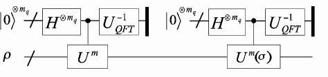
Figure 1: Circuit diagram for measuring the local density of states, consisting of two successive phase-estimation circuits on different operators. The diagonal line denotes a bundle of qubits and the thick vertical bar denotes a projective measurement of the quantum state in the computational basis. The upper register contains $m_{q}=\log(M)$ qubits and the operations on the lower register are applied conditionally $m$ times, where the integer $m\in[0,M-1]$ is determined from the binary representation of the computational basis states in the upper register.

We now describe the algorithm for estimating the LDOS on a quantum processor. The circuit for this algorithm is depicted in Fig. 1. The lower register implements the perturbed and unperturbed maps $U$ and $U(\sigma)$, requiring $n_{q}=O(\log_{2}(N))$ qubits. The upper register holds the $m_{q}=\log_{2}(M)$ ancillary qubits which fix the precision of the phase-estimation algorithm. The upper register always starts out in the ‘ready’ state $|0\rangle$. The appropriate choice of initial state $\rho$ in the $n_{q}$ register will depend on the context, as explained below. For the moment we assume the lower register is prepared in a pure state, $\rho=|\psi_{o}\rangle\langle\psi_{o}|$. The first step of the algorithm involves estimating the eigenphases of the unperturbed operator $U$. This takes the initial state through the sequence,

$$|0\rangle\otimes|\psi_{o}\rangle \rightarrow \frac{1}{\sqrt{M}}\sum_{m=0}^{M-1}|m\rangle|\psi_{o}\rangle$$ (9)

$$\rightarrow \frac{1}{\sqrt{M}}\sum_{m=0}^{M-1}|m\rangle(U)^{m}|\psi_{o}\rangle$$

$$= \frac{1}{\sqrt{M}}\sum_{m=0}^{M-1}|m\rangle\sum_{j=0}^{N-1}c_{j}\exp(i\phi_{j}m)|\phi_{j}\rangle$$

$$\rightarrow \sum_{j=0}^{N-1}c_{j}|m_{j}\rangle|\phi_{j}\rangle,$$

where $c_{j}=\langle\phi_{j}|\psi_{o}\rangle$. The state $m_{j}$ is the nearest $m_{q}$-bit binary approximation to the $j$’th eigenphase of $U$

$${\tilde{\phi}_{j}}=2\pi m_{j}/M\simeq\phi_{j}.$$ (10)

Upon strong measurement of the $m_{q}$ register one obtains and records a single outcome $m$, and the state of $n_{q}$ register must then be described by (viz, ‘collapsed to’) the updated pure state,

$$|\psi(\Delta_{m})\rangle=\sum_{\phi_{j}\in\Delta_{m}}\tilde{c}_{j}|\phi_{j}\rangle,$$ (11)

corresponding to the subspace of eigenstates with eigenphases in the band $\Delta_{m}$ of width $\Delta=2\pi/M$ about the phase $2\pi m/M$. To keep normalization the coefficients have been rescaled as follows,

$$\tilde{c}_{j}=\frac{c_{j}}{(\sum_{\phi_{j}\in\Delta_{m}}|c_{j}|^{2})^{1/2}}$$ (12)

Next we reset the $m_{q}$ qubit register to the ready state and run the phase-estimation algorithm on the operator $U(\sigma)$, producing the final state,

$$|\psi\rangle=\sum_{\phi_{j}\in\Delta_{m}}\tilde{c}_{j}\sum_{k=0}^{N-1}b(k|j)\;|m_{k}\rangle\otimes|\phi_{k}(\sigma)\rangle,$$ (13)

where ${\tilde{\phi}_{k}(l)}=2\pi m_{k}/M$ is an $m_{q}$-bit approximation to $\phi_{k}(\sigma)$. The complex coefficients $b(k|j)=\langle\phi_{j}|\phi_{k}(\sigma)\rangle$ are the inner product of the perturbed and unperturbed eigenstates. Measurement of the $m_{q}$ register now reveals an outcome $l$, associated with the eigenphases in the angular range $2\pi l/M\pm\Delta/2$. The outcome $l$ occurs with probability,

$$P_{\psi_{o}}(l|m)=\sum_{\phi_{k}\in\Delta_{l}}\left|\sum_{\phi_{j}\in\Delta_{m}}\tilde{c}_{j}\;b(k|j)\right|^{2}$$ (14)

which is conditional on the earlier outcome $m$ and the choice of initial state.

We now specify how the initial state may be chosen to eliminate unwanted fluctuations arising from the variables $\tilde{c}_{j}$ in Eq. 14 . Before describing the general solution we consider first a special case of particular interest: when a known eigenstate of $U$ may be prepared efficiently. Such an initial state may be prepared (or well approximated) by an efficient circuit when $U$ consists of some sufficiently simple integrable system (e.g., a non-interacting many-body system). In this case we have $\tilde{c}_{j}=\delta_{jk}$, and the final probability distribution Eq. 14 reduces exactly to the (coarse-grained) kernel Eq. 7,

$$P_{\phi_{k}}(l|m)\rightarrow P(\Delta_{l}|\phi_{k}).$$ (15)

When the eigenphase associated to the prepared eigenstate is known to sufficient accuracy (so that $m$ is known), it is not even necessary to perform the first phase estimation routine. In the general case of a generic quantum system, it is sufficient to prepare the maximally mixed state as the initial state, in which case the final probability distribution reduces exactly to the (coarse-grained and averaged) probability kernel Eq. 8, i.e.,

$$P_{{\bf 1}/N}(l|m)=\frac{1}{N_{m}}\sum_{\phi_{k}(\sigma)\in\Delta_{l}}\sum_{\phi_{j}\in\Delta_{m}}P(\phi_{k}(\sigma)|\phi_{j}).$$ (16)

This probability kernel contains all the information needed to compute the (coarse-grained and averaged) LDOS, $\eta_{m}(2\pi k/M)=\sum_{l}P(l|m)\delta_{k,(l-m)}$, completing our derivation.

The algorithm described above remains efficient provided that the quantum maps $U$ and $U_{\delta}$ admit Polylog($N$) gate decompositions. Such decompositions have been identified both for many-body systems with local interactions and for a wide class of few-body quantized classical models. As mentioned earlier, for practical purpose $M$ should be Polylog($N$) so the overall circuit of Fig. 1 is indeed efficient for such systems.

We now turn to the question of how many times $K$ the algorithm must be repeated to arrive at interesting physical conclusions about the final probability distribution. This issue arise because the final probability distribution is not measured directly on the quantum processor; rather, it governs the relative frequency of outcomes obtained in each repetition of the algorithm. Indeed, it is by repeating the algorithm illustrated in Fig. 1 and accumulating joint statistics of the $l$ and $m$ outputs that one can estimate the parent distribution $P(l|m)$. The accuracy of this estimation depends on the number of times $K$ the distribution is sampled. In order to bound $K$ it is convenient to cast the physical problems related to the LDOS in terms of hypothesis testing. We consider the important case of testing which of two candidates distributions $\eta_{1}$ or $\eta_{2}$ best describes the LDOS of a given system and a given perturbation. For example, one might be testing whether the Lorentzian has one of two candidate widths, or whether the profile is Gaussian or Lorentzian. Only when $K\leq\mathrm{Polylog}(N)$ will the overall computation remain efficient. This problem is resolved in general by the Chernoff bound CT1991 . A random variable is distributed according to either $P_{1}(x)$ or $P_{2}(x)$, and we wish to determine which distribution is the right one. Then, the probability $P_{e}$ that we make an incorrect inference decreases exponentially with the number of times $K$ the variable was sampled: $P_{e}\leq\lambda^{K}$. Here, $0\leq\lambda\leq 1$ is a measure of similarity between distributions defined as

$$\lambda=\min_{0\leq\alpha\leq 1}\sum_{x}P_{1}(x)^{\alpha}P_{2}(x)^{(1-\alpha)};$$ (17)

in particular, $\lambda$ is bounded above by the fidelity between $P_{1}$ and $P_{2}$. Thus, a constant error probability $\epsilon$ requires a sample of size $K=\log(\epsilon)/\log(\lambda)$. Therefore, as long as the concerned distributions are at a Polylog($N$) distance, i.e. $1-\lambda\geq 1/\mathrm{Polylog}(N)$, they can be distinguished efficiently. We note that the test can be inconclusive when both hypothesis are equally likely to describe the underlying physics.

Efficient application of the LDOS algorithm under these restrictions may be illustrated explicitly by working through a problem of practical interest from the recent literature. We consider the problem of testing whether the Breit-Wigner profile Eq. 1 applies when a given quantized classically chaotic model is subjected to a perturbation of interest. From the BGS conjecture BT77BGS84 and studies of (banded) random matrix models Wigner ; FM95 ; Jacquod95 ; FCIC96 , it is generally expected that for fully chaotic models with generic perturbations Eq. 1 applies with,

$$\Gamma(\sigma)=2\pi\sigma^{2}\rho_{E},$$ (18)

provided that the effective perturbation strength lies in the range,

$$1\ll\sigma\rho_{E}\ll\sqrt{b},$$ (19)

where $b$ is the bandwidth of the perturbation in the ordered eigenbasis of $U$ and $\rho_{E}$ is the level density. It should be stressed that $\Gamma$ may be estimated a priori if the perturbation is known Emerson02 ; FM95 ; Jacquod95 . Deviations from this hypothesis can arise for a wide variety of reasons (i.e., integrable or mixed classical dynamics in the unperturbed or perturbed system, non-generic properties of the perturbation, hidden symmetries, etc) and therefore analysis of the LDOS remains an active area of numerical study for both dynamical models BGI98 ; Wisniacki02 and real systems FGGK94 .

The lower bound of Eq. 19 is determined from the breakdown of perturbation theory and leads to a width $\Gamma$ that decreases linearly with $N$. Since the circuit can only efficiently resolve the LDOS with accuracy 1/Polylog($N$), the BW profile with width $\Gamma=O(N^{-1})$ may not be verified efficiently near this lower bound. However, near the upper bound of Eq. 19 the validity of the BW profile may be tested efficiently. In the case of fully chaotic models one has $b=N/2$ and the upper bound for $\Gamma$ is therefore $O(1)$. Hence the validity of Eq. 1 provides a hypothesis which may be tested efficiently for any perturbation such that $1/\mathrm{Polylog}(N)\ll\Gamma(\sigma)\ll O(1)$. Near this bound one can also determine whether the chaotic model exhibits dynamical localization, since in this case one has a bandwidth $b\ll N/2$ and the LDOS will cease to maintain the BW profile when $b\rho_{E}^{-1}\ll\Gamma(\sigma)\ll O(1)$. Indeed for some models the localization length $l$ of the eigenstates scales as $l\simeq O(1)$ Simone , and hence this length may be estimated using the LDOS algorithm with only Polylog($N$) resources.

In summary we have reported an algorithm for efficiently estimating the LDOS of a quantum system subject to perturbation. There is wide range of contexts in which important coarse features of the LDOS, such as the width, may be estimated with only Polylog($N$) resources. We have described in detail the important problem of testing the Breit-Wigner hypothesis as one example for which the LDOS estimation algorithm gives an effective exponential speed up over classical computation.

We are grateful to D. Shepelyanksy and Y. Weinstein for helpful discussions. This work was supported by the NSF and CMI.

References

- (1) S. Lloyd, Science 273, 23 Aug. (1996).
- (2) D. Abrams and S. Lloyd, Phys. Rev. Lett. 83, 5162 (1997).
- (3) E.P. Wigner, Ann. Math. 62, 548 (1955); 65, 203 (1957).
- (4) A. Bohr and B. Mottelson, Nuclear Structure, Vol. 1 (Benjamin, New York, 1969).
- (5) V.V. Flambaum, A.A. Gribakina, G.F. Gribakin, M.G. Kozlov, Phys Rev A 50, 267 (1994)
- (6) B. Georgeot and D.L. Shepelyansky, Phys Rev Lett 79, 4365, 1997.
- (7) V.V. Flambaum and F. Izrailev, Phys.Rev. E61 (2000) 2539.
- (8) B. Georgeot and D.L. Shepelyansky, quant-ph/0005015.
- (9) G. Benenti, Giulio Casati, Simone Montangero, Dima L. Shepelyansky, Eur. Phys. J. D 20 (2002) 293.
- (10) D. Cohen, E.J. Heller, Phys Rev Lett 84, 2841 (2000); D. Cohen, A. Barnett, E. J. Heller, PRE 63 046207 (2001); J. Vanicek and D. Cohen, quant-ph/0303103.
- (11) F. Borgonovi, I Guarneri, and F.M. Izrailev, Phys. Rev. E 57, 5291 (1998).
- (12) See for example, F. Izrailev, in Chaos and Quantum Physics, edited by A. Voros and M-J. Giannoni (North-Holland, Amsterdam, 1990).
- (13) Ph. Jacquod, P.G. Silvestrov, C.W.J. Beenakker, Phys. Rev. E 64, 055203 (2001).
- (14) J. Emerson, Y.S. Weinstein, S. Lloyd, and D. Cory, Phys. Rev. Lett. 89, 284102 (2002).
- (15) F. Cucchietti, C.H. Lewenkopf, E.R. Mucciolo, H. Pastawski and R.O. Vallejos, nlin.CD/0112015.
- (16) D. Wisniacki and D. Cohen, Phys. Rev. E 66, 046209 (2002).
- (17) Y.V. Fyodorov and A.D. Mirlin, Phys Rev B 52, 580 (1995).
- (18) Ph. Jacquod and D.L. Shepelyansky, Phys. Rev. Lett. 75, 3501 (1995).
- (19) Y.V. Fyodorov, O.A. Chubykalo, F.M. Izrailev, and G. Casati, Phys. Rev. Lett. 76, 1603 (1996).
- (20) J.L. Gruver, J. Aliaga, H.A. Cerdeira, P.A. Mellow and A.N. Proto, Phys Rev E 55, 6370 (1997).
- (21) C. Cohen-Tannoudji, J. Dupont-Roc, and G. Grynberg, Atom-photon Interactions: Basic Processes and Applications (Wiley, New York, 1992).
- (22) T. M. Cover and J. A. Thomas, Elements of Information Theory, John Wiley, New York (1991).
- (23) D. Wisniacki, E. Vergini, H. Pastawski, and F. Cucchietti, nlin.CD/0111051.
- (24) M.V. Berry and M. Tabor, Proc. Roy. Soc. Lond. A356, 375 (1977); O. Bohigas, M.J. Giannoni, C. Schmit, Phys. Rev Lett. 52, 1 (1984).
- (25) G.Casati, S.Montangero, quant-ph/0307165.