Entropic uncertainty relations for the ground state of a coupled system

Abstract

There is a renewed interest in the uncertainty principle, reformulated from the information theoretic point of view, called the entropic uncertainty relations. They have been studied for various integrable systems as a function of their quantum numbers. In this work, focussing on the ground state of a nonlinear, coupled Hamiltonian system, we show that approximate eigenstates can be can be constructed within the framework of adiabatic theory. Using the adiabatic eigenstates, we estimate the information entropies and their sum as a function of the the nonlinearity parameter. We also briefly look at the information entropies for the highly excited states in the system.

I Introduction

The uncertainty relations, that express the inability to simultaneously measure the states of two non-commuting observables, form the cornerstone of quantum physics. For any pair of operators $\widehat{A}$ and $\widehat{B}$, in standard form robert , they are stated as,

$$\Delta A~{}\Delta B\geq\frac{1}{2}\langle\Psi|[\widehat{A},\widehat{B}]|\Psi\rangle$$ (1)

where $\Delta A$ and $\Delta B$ represent the dispersions in $\widehat{A}$ and $\widehat{B}$ and $[\widehat{A},\widehat{B}]$ is the commutator. In recent years, there has been a revival of interest in the uncertainty relations reformulated from the stand point of information theory, called the entropic uncertainty relations (EUR) eur1 . For instance, the position-momentum uncertainty relation is formulated as follows; Given an eigenstate of a quantum system, $\psi(q)$ and $\widetilde{\psi}(p)$, in configuration and momentum space representations, and if $S_{q}$ and $S_{p}$ represent their information entropies, then the entropic uncertainty relations can be written down as,

$$S_{q}+S_{p}\geq S_{qp}$$ (2)

where $S_{qp}$ is the lower bound to the entropic sum or EUR. Here, the information entropy is defined as,

$$S_{\xi}=-\int^{\infty}_{-\infty}\rho(\vec{\xi})\ln\rho(\vec{\xi})~{}d\vec{\xi}$$ (3)

where $\rho(\vec{\xi})=|\psi(\vec{\xi})|^{2}$ is the probability density. The information entropy is a measure of the spreading or localisation of the given eigenstate. Apart from its intrinsic value, the reformulation also seeks to address some of the shortcomings in the standard statement of the uncertainty principle eur1 . It also quantifies the uncertainty more accurately than the standard statement based on dispersions bet . In particular, a good amount of work has focussed on obtaining the lower bounds $S_{qp}$ in general and we mention the result due to Bialynicki-Birula and Mycielski bbm ,

$$S_{q}+S_{p}\geq D(1+\ln\pi)$$ (4)

where $D$ is the dimensionality of the system. Inspired by this general result, several authors have focussed on obtaining the lower bounds for EUR of quantum systems whose classical limit is integrable, like the particle in an infinite well infw , harmonic oscillator and hydrogen atom in one and higher dimensions ho , power-law wavepackets pow and oscillating circular membrane cir . Apart from the lower bounds, the values of EUR as a function of quantum numbers has been analysed in detail in these series of papers. Recently, Dehesa et. al. have shown that for the one-dimensional power-law potentials of the form $V(x)=x^{2k}$, where $k$ is a positive integer, in the region of highly excited states, the entropic sum goes as $\ln(2n)$ for all $k$ deh .

On the other hand, the single-particle probability density $\rho(\vec{\xi})$ is also the quantity of fundamental interest in the density functional theory and hence its characterisation using information entropy as a measure for spreading has assumed special interest. In fact, treating atomic and molecular entropic sum was considered by Gadre gad1 and he derived an approximate expression for the entropic sum within the Thomas-Fermi framework for neutral atoms. Now it is known from several empirical studies for atomic, molecular and nuclear distributions that the entropic sum can be modelled as amnc ,

$$S\equiv c_{1}+c_{2}\ln N$$ (5)

where $c_{1}$ and $c_{2}$ are constants and $N$ is number of electrons or nucleons, as the case maybe. The functional form given above seems to be fairly universal for many-fermions in some mean interactions amnc .

Thus, one branch of the work on EUR has focussed on quantum systems in the classically integrable limit whose eigenstates are analytically known. The other complementary branch has explored the complex atomic and molecular systems using a combination of approximate analytical and empirical methods. In these cases, the EURs have been obtained as a function of increasing quantum numbers. However, simple and chaotic model systems that bridge this divide between the purely integrable and the complex many-body systems have not yet been considered. The main reason seems to be that, as yet, no straightforward analytical technique is available to determine their eigenstates. Thus, the main purpose of this article is to show that using adiabatic technique approximate eigenstates can be constructed and further that the entropic sums can also be estimated. In contrast to earlier works, we study the EUR as a function of the nonlinearity parameter in the system. Thus, we hope to understand the effect of nonlinearity using information theoretic measures.

In general, the non-integrable Hamiltonian systems are generic rather than an exception and model realistic physical systems. Their phase space presents a mixture of regular and irregular trajectories, whose properties change with a parameter. The evolution of the probability density as a function of the parameter reflects the influence of these classical objects. Thus it is important to look at the EUR upon variation of the nonlinearity parameter. Note that scale invariance of entropic sums leads to EURs that are independent of scaling parameters in an integrable system. But, in a non-integrable system, the entropic sums could depend on the nonlinearity parameter.

II Model Hamiltonian

In this work, we will consider the model Hamiltonian,

$$H=\frac{p_{x}^{2}}{2}+\frac{p_{y}^{2}}{2}+\frac{k_{1}^{2}x^{2}}{2}+\frac{k_{2}^{2}y^{2}}{2}+\alpha x^{2}y^{2}$$ (6)

whose potential is displayed in Fig. 1 and $k_{1},k_{2},\alpha$ are the parameters. The system is integrable for $\alpha=0$ and corresponds to two-dimensional harmonic oscillator whose asymptotic (large quantum number) entropic sum was recently derived ho . For a choice of $\alpha=0.05$ ($k_{1}=k_{2}=1$), the system displays classical chaos for energy $E>15$ cho .

Figure 1: The contours of the potential as a function of $x$ and $y$ for $\alpha=0.2$ and $k_{1},k_{2}=1$. Each contour represents a particular value of energy. For large values of energy, the potential develops ’channels’, as seen in the figure.

The coupled oscillators are popular as models of chaos since they qualitatively mimic the complex dynamics in problems like the hydrogen atom in strong fields and generalised van der Waals potential ganesan . For a generic chaotic system, most of its eigenstates could be thought of as random waves except for a small sub-set of ’regular’ states that are influenced by the nature of local classical dynamics. Hence in this work, we will only focus attention, for most part, on the ground state and, briefly, on the regular states. We stress that even though the system is chaotic, we study only those eigenstates that are associated locally with regular classical structures. Ground state is pre-eminent because previous studies have shown that the ground state saturates the EUR inequality in some systems (e.g. harmonic oscillator) and often in complex systems, the focus is on the ground state properties. Next, we obtain the ground state entropies, as a function of $\alpha$.

III Adiabatic Theory

In the context of two degrees of freedom systems, if the frequency of oscillations between both the degrees of freedom differ vastly, then such a classical system becomes an ideal candidate for the adiabatic treatment. This is the well known Born-Oppenheimer approximation in atomic physics boa . The approach is to average over the ’faster’ degree of freedom and incorporate it into the Hamiltonian for the slower degree of freedom. In this adiabatic approach, the Hamiltonian is effectively integrable and can be quantised. This has been successfully implemented earlier to estimate the energies of the localised states in coupled oscillator systems adia ; cho . For the Hamiltonian in Eq. (6), Certain and Moiseyev construct adiabatic eigenstates formally cho . Prange et. al. construct adiabatic eigenstates for a class of chaotic billiards prange .

III.1 Position Eigenstates

In this section, we will obtain the ground state of the Hamiltonian in Eq. (6), for $\alpha<<1$, in the adiabatic approximation, closely following the technique in Refs. cho ; adia . We assume that the $y$-motion is faster and average over the fast motion by dropping terms that depend purely on $x$ and $p_{x}$. This gives,

$$H^{\prime}(x;y)=\frac{p_{y}^{2}}{2}+\frac{k_{2}^{2}y^{2}}{2}+\alpha x^{2}y^{2}=E^{\prime}(y)$$ (7)

where the variable $x$ is treated as a parameter. This is just the harmonic oscillator whose frequency is

$$\Omega_{x}=\sqrt{k_{2}^{2}+2\alpha x^{2}}$$ (8)

and for $\alpha<<1$, such that $k_{2}^{2}>>2\alpha x^{2}$, then

$$\Omega_{x}\backsimeq\omega_{x}=k_{2}+\frac{\alpha}{k_{2}}x^{2}$$ (9)

The ground state of $H^{\prime}(x;y)$ for $\alpha<<1$ is,

$$\phi(x;y)=\left(\frac{\omega_{x}}{\pi}\right)^{1/4}\exp(-\omega_{x}y^{2}/2)$$ (10)

Now, the adiabatic Hamiltonian is obtained as,

$$H_{ad}=\frac{p_{x}^{2}}{2}+\frac{k_{1}^{2}x^{2}}{2}+\omega_{x}J_{y}$$ (11)

where $J_{y}$ is the classical action corresponding to the faster motion. In terms of action-angle coordinates, we get,

$$H_{ad}=J_{x}~{}~{}\sqrt{k_{1}^{2}+2\alpha J_{y}/k_{2}}+k_{2}J_{y}$$ (12)

Note that semiclassical quantisation of $H_{ad}$, which is also exact in this case, gives for the ground state energy,

$$E_{ad}=\frac{1}{2}\sqrt{k_{1}^{2}+\frac{\alpha}{k_{2}}}+\frac{k_{2}}{2}$$ (13)

The energy estimated by this formula is in good agreement with the computed energies for small $\alpha$. Since we are interested only in the eigenstate, the last term in Eq. (12) can be omitted since it only serves to shift the energy scale. The ground state of $H_{ad}$ is,

$$\psi(x)=\left(\frac{\omega}{\pi}\right)^{1/4}\exp(-\omega x^{2}/2)$$ (14)

where $\omega=\sqrt{k_{1}^{2}+\frac{\alpha}{k_{2}}}$. The ground state of the Hamiltonian in Eq. (6), for $\alpha<<1$, in the adiabatic approximation, can be written down in its characteristic form as, $\Psi(x,y)=\phi(x;y)~{}\psi(x)$, so that,

$$\Psi(x,y)=\frac{(\omega\omega_{x})^{1/4}}{\sqrt{\pi}}~{}e^{-\omega_{x}y^{2}/2}~{}e^{-\omega x^{2}/2}$$ (15)

Note that $\Psi(x,y)$ is a coupled eigenstate; the coupling provided by $\omega_{x}$. It is correctly normalised. For $\alpha=0$ it reduces to a two-dimensional harmonic oscillator wavefunction. The price we pay in the adiabatic approximation is that the eigenstate is not symmetric under $x\leftrightarrow y$ as required by the potential.

III.2 Momentum eigenstate

We calculate the eigenstate in the momentum representation by taking Fourier transform of the eigenstate given in Eq. (15). We perform the following integral,

$$\widetilde{\Psi}(p_{x},p_{y})=\frac{1}{2\pi}\int^{\infty}_{-\infty}\int^{\infty}_{-\infty}\Psi(x,y)e^{ip_{x}x}e^{ip_{y}y}~{}~{}dx~{}~{}dy$$ (16)

By a straightforward transformation of variables, we can reduce it to an one-dimensional integral,

$$\widetilde{\Psi}(p_{x},p_{y})=\frac{\omega^{1/4}}{\sqrt{2}\pi}\int^{\infty}_{-\infty}dx\frac{e^{-\omega x^{2}/2}e^{-p_{y}^{2}/2\omega_{x}}e^{ip_{x}x}}{\omega_{x}^{1/4}}$$ (17)

At this point, in order to be able to do the integration, we approximate the integrand for $\alpha<<1$. We take,

$$\exp{\left(\frac{-p_{y}^{2}}{2\omega_{x}}\right)} \backsimeq \exp{\left(\frac{-p_{y}^{2}(1-(\alpha/k_{2}^{2}))x^{2}}{2k_{2}}\right)}$$

$$\omega_{x}^{-1/4} \backsimeq \frac{1}{k_{2}}\exp\left(-\frac{\alpha}{4k_{2}^{2}}x^{2}\right)$$ (18)

Then, the integral reduces to a Fourier transform of a Gaussian,

$$\widetilde{\Psi}(p_{x},p_{y})=\frac{\omega^{1/4}}{\sqrt{2}\pi}\exp\left(\frac{-p_{y}^{2}}{2k_{2}}\right)\int^{\infty}_{-\infty}f(x)~{}~{}e^{ip_{x}x}~{}~{}dx$$ (19)

where,

$$f(x)=\exp\left(\frac{-x^{2}}{2}\omega_{p}\right)~{}~{}~{}~{};~{}~{}~{}~{}\omega_{p}=\beta-\frac{\alpha p_{y}^{2}}{k_{2}^{3}}$$ (20)

and $\beta=\omega+\alpha/2k_{2}^{2}$. This integral can be performed and we obtain the momentum eigenstate as,

$$\widetilde{\Psi}(p_{x},p_{y})=\frac{1}{\sqrt{\pi}}\left(\frac{\omega}{k_{2}}\right)^{1/4}\frac{\exp(-\frac{p_{y}^{2}}{2k_{2}})\exp(-\frac{p_{x}^{2}}{2\omega_{p}})}{\sqrt{\omega_{p}}}$$ (21)

This eigenstate is also of the product form characteristic of the adiabatic approximation, $\widetilde{\Psi}(p_{x},p_{y})=\chi_{1}(p_{x};p_{y})\chi_{2}(p_{y})$, where $\chi_{1}$ and $\chi_{2}$ represent the eigenstates of fast and slow degrees of freedom. In contrast to the position eigenstate in Eq. (15), the ground state in momentum representation is normalised only to $O(\alpha)$. This is due to the approximations that were done in the course of obtaining the Fourier transform. As a limiting case, for $\alpha=0$, it reproduces the 2D momentum eigenstate.

IV Ground state entropy

IV.1 Position Entropy

Now it is possible to evaluate the information entropies with the eigenstates in Eqs. (15,21). The position density, from Eq.(15), is given by,

$$\rho(x,y)=|\Psi(x,y)|^{2}=\frac{\sqrt{\omega\omega_{x}}}{\pi}e^{-\omega_{x}y^{2}}e^{-\omega x^{2}}$$ (22)

Then, the information entropy can be evaluated as,

$$S_{q}(\alpha,k_{1},k_{2}) = -\int^{\infty}_{-\infty}\int^{\infty}_{-\infty}\rho(x,y)\ln\rho(x,y)~{}dx~{}dy$$ (23)

$$= 1+\ln\pi-\ln\sqrt{\omega}-\frac{I_{1}}{\sqrt{\pi}}$$

where $I_{1}$ is the integral given by,

$$I_{1}=\int^{\infty}_{-\infty}e^{-x^{2}}~{}\ln\left(k_{2}+\frac{\alpha}{\omega k_{2}^{2}}x^{2}\right)~{}dx$$ (24)

Though this integral can be exactly done, we expand the integrand to first order in $\alpha$ and arrive at the following expression for the entropy valid for $\alpha<<1$,

$$S_{q}(\alpha,k_{1},k_{2})=1+\ln\pi-\ln\sqrt{k_{1}k_{2}}-\frac{\alpha}{4}\frac{k_{1}+k_{2}}{k_{1}^{2}k_{2}^{2}}+O(\alpha^{2})$$ (25)

The spatial entropy decreases linearly with $\alpha$. Setting $\alpha=0$, we recover the correct 2-dimensional harmonic oscillator entropy. In Fig 2(b) we show the spatial entropy ($k_{1}=k_{2}=1$) as a function of $\alpha$. For comparison, we numerically estimate the entropies by diagonalising the Hamiltonian in Eq. (6) in harmonic oscillator basis set and a subsequent entropy calculation. There is a good agreement between the numerical results (dots) obtained without any approximation and the analytical formula (solid line). A linear fit to the numerical entropies gives a slope of -0.4533, not far from the theoretical result -0.5. The fitted slope closely approximates -0.5 as $\alpha\to 0$.

IV.2 Momentum Entropy

The momentum density, $\widetilde{\rho}(p_{x},p_{y})$, from Eq.(21), is given by,

$$|\widetilde{\Psi}(p_{x},p_{y})|^{2}=\frac{1}{\pi}\sqrt{\frac{\omega}{k_{2}}}~{}\frac{\exp\left(-\frac{p_{y}^{2}}{k_{2}}\right)\exp\left(-\frac{p_{x}^{2}}{\omega_{p}}\right)}{\omega_{p}}$$ (26)

Once again, an entropy integral similar to Eq.(23) can be performed by Taylor expanding the denominator in the integrand to $O(\alpha)$. The final, rather cumbersome, expression turns out to be,

$$S_{p}(\alpha,k_{1},k_{2})=\sqrt{\frac{\omega/\beta}{(1-c)}}~{}\left(\frac{1}{2}-\ln\left(\frac{\sqrt{\omega/k_{2}}}{\pi\beta}\right)+\frac{(1-2c)}{2(1-c)}\right)$$ (27)

where we use the shorthand, $c=\alpha/2\beta k_{2}^{2}$. As a limiting case, we get for $\alpha=0$, the correct momentum entropy of 2D harmonic oscillator. To obtain an explicit expression, we expand to $O(\alpha)$ all the terms in the above equation. The result valid for $\alpha<<1$, is,

$$S_{p}(\alpha,k_{1},k_{2})=1+\ln\pi+\ln\sqrt{k_{1}k_{2}}+\frac{\alpha}{4}\frac{k_{1}+k_{2}}{k_{1}^{2}k_{2}^{2}}+O(\alpha^{2})$$ (28)

This expression shows that the momentum entropy increases linearly with $\alpha$. This is evident from Fig 2(a) in which a good agreement is seen between the numerical and the analytical result. A linear fit gives the slope to be 0.4765, close to the expected value 0.5.

Figure 2: Entropy for the ground state of the Hamiltonian in Eq. (6) with $k_{1}=k_{2}=1$ as a function of $\alpha$. (a) Momentum entropy and (b) spatial entropy. Dots are numerical values of information entropies obtained without any approximation. Continuous lines are theoretical curves of Eqs. (25,28)

Figure 3: Entropy sum for the ground state of the Hamiltonian in Eq. (6) with $k_{1}=k_{2}=1$ as a function of $\alpha$. Dots are numerical values and continuous line is the quadratic fit to the numerical data.

IV.3 Entropic sum

From the entropy expressions in Eqs. (25,28), we obtain the sum of position and momentum entropies as,

$$S(\alpha)=S_{q}+S_{p}=2~{}(1+\ln\pi)+O(\alpha^{2})$$ (29)

We point some salient features of this result. To $O(\alpha)$, the entropic sum is invariant under change of $\alpha$, but definitely satisfies the uncertainty inequality in Eq. (4). As expected, due to the scale invariance, it is also independent of the parameters $k_{1}$ and $k_{2}$. However, as revealed by numerical computations in Fig 3, the significant contribution to entropic sum comes from terms of $O(\alpha^{2})$, which could not be determined from the present method. The important result is that, for $\alpha<<1$, the entropies and their sum depend only on the parameter $\alpha$, infact on terms of $O(\alpha^{2})$ or higher. Since our method does not yield information on the quadratic and higher order $\alpha$ terms, we perform a fit to the numerical entropic sum. The equation of best fit, for the range of $\alpha$ considered, gives $S=4.289+0.063\alpha+0.466\alpha^{2}$. As expected, the fitted equation shows that the linear term in $\alpha$ carries less weight and the intercept is a good approximation to $2(1+\ln\pi)$. The ground state saturates the entropic sum only for $\alpha=0$.

The role of $\alpha$, primarily, is to change the shape of the potential which leads to other qualitative changes in the classical dynamics of the system. As $\alpha$ increases, the potential develops ’channels’ (see Fig. 1) but the ground state does not occupy the channels. The potential restricts the ground state to remain within the central region and not expand into the channels of the potential. Hence the spatial entropy decreases with increase in $\alpha$ indicating stronger localisation of the ’particle’ near the origin of the potential. Correspondingly, the momentum entropy increases. But they do not cancel one another exactly, and the increase in entropic sum is of the order $O(\alpha^{2})$. Thus, it is a rather slow but definite increase, as evident from Fig. 3.

V Large Parameter

We note that the limit $\alpha\to\infty$ is a singular limit for the Hamiltonian in Eq. (6). It does not seem feasible to extend the present method to this limit. Hence we look at $\alpha>>1$, but not $\alpha\to\infty$.

V.1 Position Eigenstate

For $\alpha>>1$, we cannot Taylor expand as done in Eq. (9). Hence, now the adiabatic Hamiltonian will be,

$$H_{ad}=\frac{p_{x}^{2}}{2}+\frac{k_{1}^{2}x^{2}}{2}+\Omega_{x}J_{y}$$ (30)

Presently, exact solutions are not known for this problem. To go further, we quantise the $y$ degree of freedom exactly and treat the $x$ degree of freedom using the variational method. This leads to,

$$H_{ad}=\frac{p_{x}^{2}}{2}+\frac{k_{1}^{2}x^{2}}{2}+\frac{1}{2}\sqrt{k_{2}^{2}+2\alpha x^{2}}$$ (31)

where $\Omega_{x}$ is substituted from Eq.(8). Now, we will use variational method to obtain the ground state. The trial wavefunction of the form,

$$\psi_{tr}(x)=\left(\frac{b}{\pi}\right)^{1/4}\exp(-bx^{2}/2)$$ (32)

is assumed. Note that the trial wavefunction is similar to the adiabatic ground state in Eq. (14), except for $\omega$ being replaced by the variational parameter $b$, to be determined. Since we are applying the standard variational technique as expounded in many quantum physics books, we refer the reader to, say tan , for details of the variational method. We first determine the energy functional,

$$E_{v} = \langle\psi_{tr}(x)\mid H_{ad}\mid\psi_{tr}(x)\rangle$$ (33)

$$= \frac{b}{4}+\frac{k_{1}^{2}}{4b}+\sqrt{\frac{\alpha}{2b}}\;\;U(-1/2,0,bk_{2}^{2}/2\alpha)$$ (34)

where $U(,,)$ is the confluent Hypergeometric function. Now, we optimise $E_{v}$ to obtain $b$. Hence,

$$\frac{dE_{v}}{db} = \frac{1}{4}-\frac{k_{1}^{2}}{4b^{2}}+\frac{e^{bk_{2}^{2}/4\alpha}\;k_{2}^{2}\;K_{0}(bk_{2}^{2}/4\alpha)}{4\sqrt{2b\pi\alpha}}$$ (35)

$$-\frac{\sqrt{\alpha}}{2\sqrt{2}b^{3/2}}\;U(-1/2,0,bk_{2}^{2}/2\alpha)$$

where $K_{0}(.)$ is the modified Bessel function of second kind.

Now, we solve for $b$ by setting $dE_{v}/db=0$. Once again, solving for $b$ in a general case does not seem feasible. However, in the limit $\alpha>>1$, we use the asymptotic forms as $z=(bk_{2}^{2}/2\alpha)\to 0$ asymp ,

$$U\left(\frac{-1}{2},0,z\right) \thicksim \frac{1}{\sqrt{\pi}}\left(1+\frac{z}{2}\left(\ln z+\Psi(\frac{1}{2})+2\gamma-1\right)\right)$$

$$K_{0}(z/2) \thicksim -\ln(z/2)$$ (36)

where $\gamma=0.5772...$ is the Euler’s constant and $\Psi(.)$ is the digamma function. We use these asymptotic forms and ignore terms that contain $\alpha$ in the denominator. Then, we obtain,

$$\frac{dE_{v}}{db}\simeq\frac{1}{4}-\frac{k_{1}^{2}}{4b^{2}}-\frac{\sqrt{\alpha}}{2\sqrt{2\pi}b^{3/2}}=0$$ (37)

If the terms are rearranged, this turns out to be a quartic algebraic equation in $b$.

$$b^{4}-2k_{1}^{2}b^{2}-\frac{2\alpha b}{\pi}+k_{1}^{4}=0$$ (38)

This can be exactly solved for $b$ but leads to rather complicated terms. As an aside, we also point out that using asymptotic forms for $U(.)$ and $K_{0}(.)$ as $z\to\infty$, i.e, $\alpha\to 0$, we can recover the position eigenstate obtained in Eq. (15).

From this point, we specialise to our case $k_{1}=k_{2}=1$. Then, for $\alpha>>1$, the second term in Eq. (38) can be neglected since $b$ increases monotonously with increasing $\alpha$. Now, setting $dE_{v}/db=0$, we obtain for $\alpha>>1$,

$$b\approx\left(\frac{2\alpha}{\pi}\right)^{1/3}$$ (39)

In general, $b$ is dependent on $k_{1}$ and $k_{2}$ as evident from the exact solution to Eq. (38) but we have taken $k_{1}=k_{2}=1$. Plugging in this $b$ in Eq. (32), we obtain the adiabatic ground state valid for $\alpha>>1$ as,

$$\Psi(x,y)=\frac{(b\Omega_{x})^{1/4}}{\sqrt{\pi}}~{}e^{-\Omega_{x}y^{2}/2}~{}e^{-bx^{2}/2}$$ (40)

where $\Omega_{x}=\sqrt{1+2\alpha x^{2}}$ since we have taken $k_{1}=k_{2}=1$ to make the analysis tractable. It is correctly normalised but does not give the correct limit for $\alpha=0$. It does not possess the symmetry $x\leftrightarrow y$.

V.1.1 Position entropy for $\alpha>>1$

The probability density in position representation is,

$$\rho(x,y)=|\Psi(x,y)|^{2}=\frac{\sqrt{b\Omega_{x}}}{\pi}e^{-\Omega_{x}y^{2}}e^{-bx^{2}}$$ (41)

From this, the information entropy with $k_{1}=k_{2}=1$ can be evaluated (see Eq. (23) as,

$$S_{q}(\alpha)=1+\ln\pi-\ln\sqrt{b}-\frac{I_{2}}{\sqrt{\pi}}$$ (42)

where $I_{2}$ is given by,

$$I_{2} = \int^{\infty}_{-\infty}e^{-x^{2}}~{}\ln\left(1+\frac{2\alpha}{b}x^{2}\right)~{}dx$$ (43)

$$= \sqrt{\pi}\left[\gamma+\pi~{}\mbox{erfi}\left(\sqrt{\frac{b}{2\alpha}}\right)+\ln\left(\frac{\alpha}{2b}\right)-\right.$$

$$\left.\frac{b}{\alpha}_{\phantom{1}2}F_{2}\left(1,1;\frac{3}{2},2;\frac{b}{2\alpha}\right)\right]$$

and $\mbox{erfi}(.)$ is the imaginary error function and ${}_{\phantom{1}2}F_{2}(.)$ is the generalised hypergeometric function. In this form, the information entropy in Eq. (42) is not particularly illuminating. For $\alpha>>1$, the contributions from 2nd and 4th term in Eq. (43) is negligible. Thus, we obtain a simplified form for the spatial entropy,

$$S_{q}(\alpha)=1+\ln\pi-\ln\sqrt{b}+\frac{\gamma}{4}-\frac{1}{4}\ln\left(\frac{\alpha}{2b}\right)$$ (44)

Now, substituting for $b$ from Eq. (38), we obtain,

$$S_{q}(\alpha)=1+\ln\pi+\frac{\gamma}{4}-\frac{1}{3}\ln\left(\frac{\pi}{2}\right)-\frac{1}{3}\ln\alpha$$ (45)

Thus, for large $\alpha$, the ground state entropy falls logarithmically with a slope 1/3. This is verified numerically through exact calculations. In Fig. 4(b), we show the position entropy plotted as a function of $\ln(\alpha)$. A linear regression gives the best fit line as $S_{q}=2.1368-0.3033\ln\alpha$, verifying the approximate theoretical slope in Eq. (45). The intercept is approximately $1+\ln\pi$, the entropy of the unperturbed oscillator, but we stress that we cannot recover $\alpha=0$ result from Eq. (45). We also point out a systematic difference seen in Fig. 4(a,b) between the theoretical estimate of entropy (crosses) given by Eq. (45) and the numerical result (circles). This is due to the adiabatic approximation becoming less accurate near the origin of the potential and this is showing up in the results.

V.2 Momentum eigenstate and entropy

We obtain adiabatic ground state in the momentum representation for $\alpha>>1$ by Fourier transforming the position eigenstate in Eq. (40). We need to perform the integral in Eq. (16) using the ground state in Eq. (40). Once again, by transforming variables, we can reduce it to a one-dimensional integral,

$$\widetilde{\Psi}(p_{x},p_{y})=\frac{b^{1/4}}{\sqrt{2}\pi}\int^{\infty}_{-\infty}dx\frac{e^{-bx^{2}/2}e^{-p_{y}^{2}/2\Omega_{x}}e^{ip_{x}x}}{\Omega_{x}^{1/4}}$$ (46)

where $\Omega_{x}$ is given by Eq. (8) and $b$ is the variational parameter determined in Eq. (38). This integral could only be performed numerically. Hence, we first determine the adiabatic momentum eigenstate by numerically integrating Eq. (46) from which the entropies are computed. The entropies obtained numerically by the adiabatic approach, shown as crosses in Fig 4(a), and those obtained numerically without any approximation (circles in Fig 4(a)) are in fair agreement with each other for the range of $\alpha$ considered in this work. A linear regression gives the line of best fit,

$$S_{p}(\alpha)=2.1754+0.3134\ln\alpha$$ (47)

Momentum entropy increases logarithmically with $\alpha$. We notice from our numerical calculations, exact as well as the one based on adiabatic approach, that the slope in the equation of best fit for the momentum entropy is consistently higher than the one for the position entropy. This difference accounts for the behaviour of the entropic sum presented in the next section.

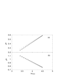
Figure 4: (a) Entropy in momentum representation and in (b) spatial representation for the Hamiltonian in Eq. (6) with $k_{1}=k_{2}=1$ as a function of $\alpha$ ranging from 30 to 90. Dots are the numerical entropies and solid line is the best fit to the numerical data. Crosses represent the theoretical result based on the adiabatic approach.

V.3 Entropic sum for large $\alpha$

Finally, we put together the results to look at the entropic sum for large $\alpha$. The Fig 5 shows the entropic sum for the ground state for a range of parameters $\alpha=30,....90$. The best fit line (solid line) is given by,

$$S=4.3249+0.00708\ln\alpha$$ (48)

Firstly, it satisfies the entropic uncertainty inequality in Eq. (4). The positive slope in this equation shows that the entropic sum increases with the parameter but rather slowly. It must also be pointed out that this slope in Eq. (48) corresponds closely to the difference in slopes corresponding to the best fit equations for position and momentum entropy.

The functional form of Eq. (48) is quite analogous to the entropic sum in Eq. (5) conjectured for atoms, clusters and nuclei gad1 ; amnc on the basis of theoretical arguments and numerical results. Such logarithmic increase in entropic sum is noted earlier for 1D power-law potentials in the semiclassical limit deh . Thus, this result provides an approximate (semi-)thereotical approach to see the emergence of the functional form in Eq. (48) in a simple coupled system.

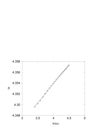
Figure 5: (a) Entropy sum for the ground state of the Hamiltonian in Eq. (6) with $k_{1}=k_{2}=1$ as a function of $\alpha$. Circles are numerical values and solid line is the best fit to the numerical data as given by the Eq. (48).

VI Highly Excited States

In this section, we look at the grey areas that are not yet clearly understood. We briefly discuss the EUR for the highly excited states. Most eigenstates of chaotic systems in the semiclassical limit are irregular or random looking states that could be modelled by random matrix theory rmt . Such random matrix averages represent a particular limit at which the system’s entropy becomes independent of the nonlinearity parameter. Hence we focus our attention on the highly excited ’regular’ states which are characterised by $N$ quanta of excitation in one degree of freedom and 0 in the other, often called the Born-Oppenheimer type of states prange ; adia . Thus they could be approximately labelled by the quantum number pair $(N,0;\alpha=\alpha_{0})$, where $N>>1$ mss1 . For these states, we will numerically explore the variation of entropies as a function of $\alpha$. In a sense, the entropies of highly excited states have already been reported before in a different context mss . Firstly, we choose a particular eigenstate characterised by $(N,0;\alpha_{0})$ , in our case (110,0;0.0), and then follow the eigenstate as a function of $\alpha$. The calculations are also somewhat cumbersome and hence we sample only a small parametric window.

Figure 6: Spatial (circle) and momentum (square) entropy for a highly excited state characterised by approximate quantum number pair (110,0) with $k_{1}=k_{2}=1$ as a function of $\alpha$.

The results, obtained from exact numerical basis-set diagonalisation and then a subsequent entropy calculation, shown in the Fig. 6 reveal that the spatial and momentum entropies display similar trend as a function of $\alpha$. This is qualitatively different from that of the ground state. From the figure, it is also clear that the variation with $\alpha$ is not monotonous. The entropic sum evidently obeys the inequality in Eq. (4). It is known that for Hamiltonian in Eq. (6) there are certain special periodic orbits which are responsible for supporting regular states in the system anc . The probability density structures are related to the classical phase space structures bebo and hence the information entropy is also intimately connected to the properties of the local classical phase space structures that support such regular states. Thus the entropy is modulated by the qualitative nature of local classical dynamics as a function of $\alpha$ mss1 .

VII Conclusions and Discussions

This work can be broadly divided into two parts. Focussing on the ground state of a coupled system, firstly, we show, within the framework of adiabatic theory, that spatial and momentum eigenstates can be constructed. Secondly, using the adiabatic eigenstates we obtain approximate results for the entropic uncertainty relations. For the ground state, we show that the spatial entropy decreases as a function of the coupling parameter $\alpha$ in the system while the momentum entropy increases. However, the entropic sum increases with the coupling parameter $\alpha$ and gets saturated only for $alpha=0$. This is reminiscent of the results reported numerically for the entropic sums of atoms, molecules and clusters amnc . Thus, this work provides an approach to obtain analytical results for the information entropies and their sums, for coupled nonlinear systems as a function of coupling parameter.

However, for highly excited states, the spatial and momentum entropy qualitatively look similar and seem to be related to the qualitative nature of local classical dynamics. In general, the relation between the classical phase space structures and the quantum eigenstates is not completely understood yet. In this context, one might mention the semiclassical approaches due to Berry and Bogomolny bebo based on the Gutzwiller’s Trace Formula. Thus, we only point out the intricacies involved in the entropic sums for the highly excited states. In due course, it might become possible to relate information entropy to classical orbits through these approaches. There are already empirical results pointing to this connection mss1 .

The adiabatic theory based approach presented here is not without demerits. Strictly speaking, the adiabatic effects take over when there is clear separation in the time-scales of motion in the two modes that constitute the system. Thus, in the case of Hamiltonian in Eq. (6), the potential develops channels (see Fig. 1) for large values of $\alpha$ and thus facilitates adiabatic effects. The adiabatic theory is particularly suitable if the probability density develops structures within these channels, as it happens for some of the highly excited states. Since the ground state does not enter the channel for large $\alpha$, it is likely to become less accurate for very large values of $\alpha$. Further, this work leaves an interesting question unanswered. What happens in the limit $\alpha=\infty$ ? The present method of treatment does not seem adequate to answer this question. We hope the results here could stimulate research on more rigorous approaches to entropic sums in a wide variety of coupled systems.

References

- (1) H. P. Robertson, Phys. Rev., 34 163 (1929).
- (2) J. S. Dehesa et. al., J. Comput. Appl. Math. 133 23 (2001) ; V. Majernik and L. Richterek, Eur. J. Phys. 18 79 (1997)
- (3) M. J. W. Hall, Phys. Rev. A 59 2602 (1999).
- (4) I. Bialynicki-Birula and J. Mycielski, Comm. Math. Phys. 44 129 (1975).
- (5) V. Majernik and L. Richterek, J. Phys. A : Math. Gen. 30 L49 (1997).
- (6) R. J. Yanez, W. Van Assche and J. S. Dehesa, Phys. Rev. A, 50 3065 (1994); W. Van Assche, R. J. Yanez and J. S. Dehesa, J. Math. Phys. 36 4106 (1995); M. W. Coffey, J. Phys. A : Gen. Math, 36 7441 (2003).
- (7) S. Abe et. al., Phys. Lett. A 295 74 (2002).
- (8) J. S. Dehesa et. al., Int. J. Bifur. Chaos. 12 2387 (2002).
- (9) J. S. Dehesa et. al., Phys. Rev. A 66 062109 (2002).
- (10) S. R. Gadre, Phys. Rev. A, 30 620 (1984).
- (11) S. E. Massen and C.P.Panos, Phys. Lett. A 246 530 (1998); J. C. Angulo, J. Phys. A: Math. Gen. 26 6493 (1993).
- (12) P. R. Certain and N. Moiseyev, J. Chem. Phys. 86 2146 (1987)
- (13) K. Ganesan and M. Lakshmanan, Phys. Rev. Lett, 62 232 (1989).
- (14) Ira N. Levine, Molecular Spectroscopy (John Wiley, 1975).
- (15) C. C. Martens et. al., J. Chem. Phys., 90 2328 (1989); J. Zakrzewski and R. Marcinek, Phys. Rev. A, 42 7172 (1990)
- (16) R. E. Prange et. al., Physica Scripta T90 134 (2001).
- (17) C. Cohen-Tannoudji, B. Diu, F. Laloe, Quantum Mechanics (Wiley, New York) (1997).
- (18) Frank W. J. Olver, Asymptotics and Special Functions, (A.K.Peters Ltd, Massachusettes, 1997).
- (19) K. R. W. Jones, J. Phys. A 23 L1247 (1990); K. Muller et. al. Phys. Rev. Lett. 78 215 (1997).
- (20) M. S. Santhanam et. al., Phys. Rev. E, 57 345 (1998).
- (21) M. S. Santhanam et. al., Mol. Phys. 88 325 (1996).
- (22) J. L. Anchell, J. Chem. Phys., 92 4342 (1990).
- (23) M. V. Berry, Proc. R. Soc. Lond A 423 219 (1989); E. B. Bogomolny, Physica D 31 169 (1988).